Fastest Learning in Small-World Neural Networks
Abstract
We investigate supervised learning in neural networks. We consider a multi-layered feed-forward network with back propagation. We find that the network of small-world connectivity reduces the learning error and learning time when compared to the networks of regular or random connectivity. Our study has potential applications in the domain of data-mining, image processing, speech recognition, and pattern recognition.
I Introduction
The concept of small-world networks and the variant of scale free networks has become very popular recently Watts98 ; Albert99 ; Barabasi99 ; Huberman99 ; Albert00 ; Jeong00 ; Kleinberg00 ; Strogatz01 ; Watts02 , after the discovery that such networks are realized in diverse areas as the organization of human society (Milgram’s experiment) Watts98 , in the WWW Albert99 ; Huberman99 , in the internet Faloutsos99 , in the distribution of electrical power (western US) Watts98 , and in the metabolic network of the bacterium Escherichia coli Strogatz01 ; Wagner01 .
According to Watts and Strogatz, a small-world network is characterized by a clustering coefficient and a path length Watts98 . The clustering coefficient measures the probability that given node is connected to nodes and then also nodes and are connected. The shortest path length from node to node is the minimal number of connections needed to get from to . A small-world network is defined by two properties. First, the average clustering coefficient is larger than for a corresponding random network with the same number of connections and nodes. The clustering coefficient expected for a regular rectangular grid network is zero while for a random network the probability of connection of two nodes is the same for neighboring nodes as for distant nodes. Second, the average path length scales like , where is the number of nodes. For regular (grid) networks scales as where is the dimension of the space and for random networks scales as . As result, is large and is small in a small-world network.

In studies of small-world neural networks it has turned out that this architecture has potentially many advantages. In a Hodgkin-Huxley network the small-world architecture has been found to give a fast and synchronized response to stimuli in the brain Corbacho00 . In associative memory models it was observed that the small-world architecture yields the same memory retrieval performance as randomly connected networks, using only a fraction of total connection length Bohland01 . Likewise, in the Hopfield associative memory model the small-world architecture turned out to be optimal in terms of memory storage abilities Labiouse02 . With a integrate-and-fire type of neuron it has been shown Sola04 that short-cuts permit self-sustained activity. A model of neurons connected in small-world topology has been used to explain short bursts and seizure-like electrical activity in epilepsy Netoff04 . In biological context some experimental works seem to have found scale-free and small-world topology in living animals like in the macaque visual cortexSporns00 , in the cat cortex Sporns00 and even in networks of correlated human brain activity measured via functional magnetic resonance imaging Dante04 . The network of cortical neurons in the brain has sparse long ranged connectivity, which may offer some advantages of small world connectivity Laughlin03 .
II Model and geometry of network
In the present work we study supervised learning with back-propagation in a multi-layered feed-forward network. Around 1960, the Perceptron model Rosenblatt62 has been widely investigated. The information (representing action potentials propagating in axons and dendrites of biological neurons) feeds in forward direction. The Perceptron model has been extended to include several layers. E.g., a convolutional network, consisting of seven layers plus one input layer has been used for reading bank cheques LeCun98 . The task of learning consists of finding optimal weights between neurons (representing synaptic connections) such that for a given set of input and output patterns (training patterns) the network generates output patterns as close as possible to target patterns. We used the algorithm of back propagation Rummelhart86 to determine those weights. There are alternative, potentially faster methods to determine those weights like, e.g. simulated annealing. Here we aim to compare different network architectures with respect to learning, using as reference a standard algorithm to determine those weights.
| R | S | |||||||
| 5 | 5 | 25 | 100 | 19 5 | 2.61 .02 | 0.19 .05 | 0.38 .02 | 0.81 .01 |
| 5 | 8 | 40 | 175 | 28 5 | 3.25 .02 | 0.17 .02 | 0.34 .06 | 0.88 .01 |
| 10 | 10 | 100 | 900 | 400 100 | 3.40 .01 | 0.44 .11 | 0.30 .02 | 0.74 .002 |
| 15 | 8 | 120 | 1575 | 830 50 | 3.20 .01 | 0.53 .03 | 0.29 .003 | 0.67 .002 |
| 15 | 15 | 225 | 3150 | 2300 300 | 3.75 .01 | 0.73 .09 | 0.29 .01 | 0.69 .002 |
We change the architecture of neural connections from regular to random architecture, while keeping the number of connections fixed. Initially, neurons are connected feed-forward, i.e. each neuron of a given layer connects to all neurons of the subsequent layer. We make a random draw of two nodes which are connected to each other. We cut that ”old” link. In order to create a ”new” link, we make another random draw of two nodes. If those nodes are already connected to each other, we make further draws until we find two unconnected nodes. Then we create a ”new” link between those nodes. Thus we conserve the total number of links. The number of links in a regular network is given by , where denotes the number of neurons per layer and denotes the number layers. In this way we create some connections between nodes in distant layers, i.e. short-cuts and the topology changes gradually (see Fig.[1]). In particular, while the initial connectivity is regular, after many rewiring steps the topology becomes random. Somewhere in between lies the small-world architecture Watts98 . We consider networks consisting of one input layer, one output layer and one or more hidden layers. While the standard Perceptron model has only two layers, here we explore the use of more hidden layers, because only then the path length can become small and the network ”small-world”.
Instead of measuring the network architecture by the functions and , we have used the functions of local and global connectivity length and , respectively, introduced by Marchiori et al. Latora ; Marchiori00 . Those functions are more suitable because they allow to take into account the connectivity matrix and the weight matrix in networks and also to treat networks with some unconnected neurons (often nodes are unconnected due to rewiring). and are defined via the concept of global and local efficiency Latora ; Marchiori00 . For a graph its efficiency is defined by
| (1) |
where denotes the shortest path length between vertices and and is the total number of vertices. Moreover, one defines the local efficiency as average efficiency of subgraphs (the subgraph is usually formed by the neurons directly connected to neuron . We have included also all neurons occuring in the same layer as neuron ).
| (2) |
The connectivity length is defined by the inverse of efficiency,
| (3) |
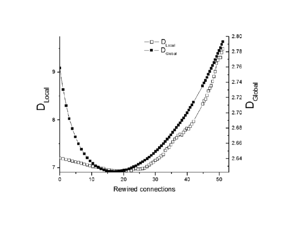
It has been shown that is similar to , and is similar to Marchiori00 , although this is not an exact relation. Thus, if a network is small-world, both, and should become small. Fig.[2] shows and as a function of the number of rewiring steps for a network of 5 neurons per layer and 5 layers. One observes that both, and , become small at about . The position of minima for other networks are shown in Tab.[1].
Small world networks are characterized by the scaling law . From the similarity of and , we expect
| (4) |
In Tab.[1] we display , where denotes the value of at the position where both and are small. The onset of scaling is observed when networks become larger. From our data we observed another scaling law for the variable . Our data are consistent with
| (5) |
where and are constants. In Tab.[1] we display . This law says that the number of rewirings associated with the minimum of and , i.e. small world connectivity, measured in terms of the number of connections of the regular network, increases with the number of connections in a logarithmic way.
III Learning
We trained the networks with random binary input and output patterns. Our neurons are sigmoid real-valued units. The learning time, defined as the number of iterations it takes until the error of training becomes smaller than a given error tolerance, depends on the error tolerance. In the following we will present the learning error instead of learning time.
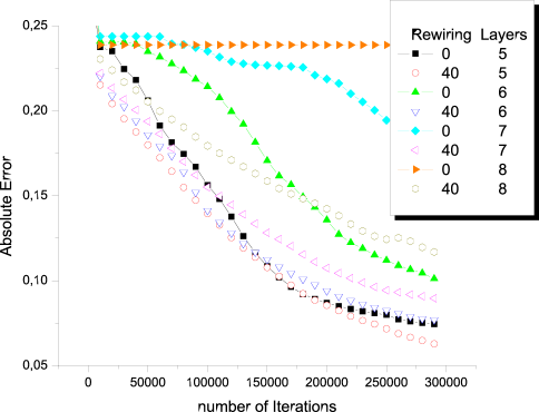
The effect on learning due to a variation of the number of layers and the effect of rewiring, i.e. introducing short-cuts, is shown in Fig.[3]. It shows the absolute error, which is an average of the absolute error over the neurons, patterns and statistical tests. We have considered a network of 5 neurons per layer and varied the number of layers from 5 to 8. We compare the regular network () with the network of . We find that for up to a few thousand iterations the network with gives a smaller error compared to the regular network. In the regime of many iterations, one observes that the 5-layer regular network learns (i.e. the error decreases with iterations), while the regular 8-layer network does not learn at all. In contrast, after 40 rewirings all networks do learn. The improvement over the regular network is small for 5 layers, but major for 8 layers. This indicates that the learning improvement due to small-world architecture becomes more efficient in the presence of more layers. In the case of 8 layers, the error curve for is in the regime where and are both small (see Tab.[1]), i.e. close to the small-world architecture.
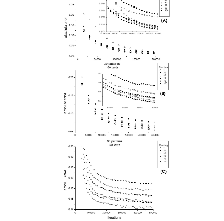
The effect on learning when changing the number of learning patterns and the rewiring of the network is shown in Fig.[4] for a network of 5 neurons per layer and 5 layers. When learning 5 patterns (Fig.[4a]) in the domain of few iterations (1000-5000), rewiring brings about a substantial reduction in the error compared to the regular network () and also to the random network (). For very many iterations (about 500000) there is little improvement with rewirings compared to the regular architecture. For learning of 20 patterns (Fig.[4b]) the behavior is similar, but the reduction of error in the presence of 20 rewirings is more substantial for many iterations. When learning 80 patterns Fig.[4c] we see that the error is large, we are near or beyond the storage capacity. In this case the regular architecture is optimal and rewiring brings no advantage.
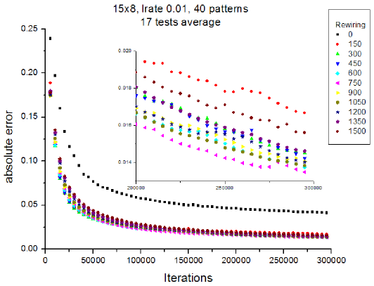
The influence of the number of neurons per layer on learning is depicted in Fig.[5]. We compare (a) a network of 5 neurons per layer and 8 layers with a network (b) of 15 neurons per layer and 8 layers. We trained the network with 40 patterns in both cases. In case (a) (not shown) we found that the error as function of rewiring has a minimum at which is in coincidence with the minimum of and given in Tab.[1], i.e in the small-world regime. This gives a clear improvement over the regular architecture () and the random architecture (). In case (b) the learning error is shown in Fig.[5]. One observes that the learning error has a minimum at , which is close to the minimum of and at (see Tab.[1]), also near the small-world regime.
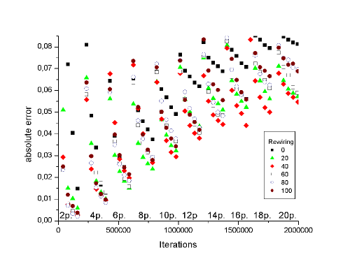
So far we studied learning when the training patterns were given all together in the beginning. However, sometimes one is interested in changing strategies or parameters during training (enforced learning). In order to see if the small world architecture gives an advantage in such scenarios, we studied learning by adding patterns sequentially in groups of 2 patterns. For a network of 5 neurons per layer and 5 layers, Fig.[6] shows the learning error versus the number of rewirings. Also here one observes a distinctive gain by introducing some rewirings (optimum at ) over the regular network () and the random network ().
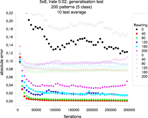
In the last experiment we studied generalization in a network of 5 neurons per layer and 8 layers. We trained the network to put patterns into classes. We considered 5 classes: A pattern belongs to class 1, if neuron 1 in the input layer has the highest value of all neurons in this layer. Class 2 corresponds to neuron 2 having the highest value. etc. The classification of 200 patterns achieved by the network as function of connectivity is shown in Fig.[7]. It turns out the network with some rewirings gives improvement over the regular and also random network architecture. We observe that the generalization error has a minimum at , which is in the regime where and are small (see Tab.[1]), i.e. in the regime of small-world architecture.
In summary, we observed that the network with some rewirings., i.e. short-cuts, gives reduced learning errors. The minimum of the error as function of rewiring lies in the neighborhood of the minimum of and which indicates small-world architecture. However, while and depend only on the connectivity of the network, learning error and learning time depend on other parameters like the number of learning patterns, or the mode of learning, e.g. standard learning or enforced learning. We believe that our results have important implications on artificial intelligence and artificial neural networks. Neural networks are being widely used as computational devices for optimization problems based on learning in applications like pattern recognition, image processing, speech recognition, error detection, and quality control in industrial production, like of car parts or sales of air-line tickets. Our study reveals a clear advantage and suggests to use small-world networks in such applications. Our study may have potential applications in the domain of data-mining.
Acknowledgements
This work has been supported by NSERC Canada. H.K. is grateful for
discussions with Y. DeKoninck, A. Destexhe and M. Steriade.
References
- (1) Watts, D.J. & Strogatz, S.H. Nature 393, 440-442 (1998).
- (2) Albert, R., Jeong, H. & Barabási, A.L. Nature 401, 130-131 (1999).
- (3) Barabási, A.L. & Albert, R. Science 286, 509 (1999).
- (4) Albert, R., Jeong, H. & Barabási, A.L. Nature 406, 378-382 (2000).
- (5) Jeong, H., Tombor, B., Albert, R., Oltvai, Z.N. & Barabási, A.L. Nature 407, 651-654 (2000).
- (6) Huberman, B.A. & Adamic, L.A. Nature 401, 131 (1999).
- (7) Kleinberg, J.M. Nature 406, 845 (2000).
- (8) Strogatz, S.H. Nature 410, 268-276 (2001).
- (9) Watts, D.J., Dodds P.S. & Newman, M.E.J. Science 296, 1302 (2002).
- (10) Faloutsos, M., Faloutsos, P. & Faloutsos, C. Comp. Comm. Rev. 29, 251-262 (1999).
- (11) Wagner, A. Proc. R. Soc. London B268, 1803-1810 (2001).
- (12) Corbacho, H.R., Lago-Fernández, F., Sigüenza, L.F. & Sigüenza, J.A. Phys. Rev. Lett. 84, 2758-2761 (2000).
- (13) Bohland, J.W.& Minai, A.A. Neurocomputing 38-40, 489-496 (2001).
- (14) Labiouse, C.L, Salah, A.A.& Starikova,I., ”The impact of connectivity on the memory capacity and the retrieval dynamics of Hopfield-type networks,” in Proceedings of the Santa Fe Complex Systems Summer School, pp. 77-84, Budapest, NM: SFI, 2002.
- (15) Rosin, A., Riecke, H., & Solla, S.A. Phys. Rev. Letters 92, 19 (2004).
- (16) Netoff, T.I, Clewley, R., Arno, S., Keck, T. & White, J.A. J. Neurosci 24, 8075-8083 (2004).
- (17) Sporns, O., Tononi, G., & Edelman, G.M. Cerebral Cortex 10, 127-141 (2000).
- (18) Dante R. Chialvo, Physica A340, 756-765 (2004).
- (19) Laughlin, S.B. & Sejnowski, T.J. Science 301, 1870-1874 (2003).
- (20) Rosenblatt, F. Principles of Neurodynamics, Spartan, New York (1962).
- (21) LeCun, Y., Bottou, L., Bengio, Y. & Haffner, P. Proc. of the IEEE 86, 2278-2324 (1998).
- (22) Rummelhart, D.E., Hinton, G.E. & Williams, R.J. Nature 323, 533-536 (1986).
- (23) V. Latora, M. Marchiori Phys. Rev. Lett. 87, 198701 (2001).
- (24) Marchiori, M. & Latora, V. Physica A285, 539-546 (2000).