Abstract

Several studies on real complex networks from different fields as biology, economy, or sociology have shown that the degree of nodes (number of edges connected to each node) follows a scale-free power-law distribution like $P(k)\approx k^{-\gamma}$, where $P(k)$ denotes the frequency of the nodes that are connected to $k$ other nodes. Here we have carried out a study on scale-free networks, where a line graph transformation (i.e., edges in an initial network are transformed into nodes) is applied to a power-law distribution. Our results indicate that a power-law distribution as $P(k)\approx k^{-\gamma+1}$ is found for the transformed network together with a peak for low-degree nodes. In the present work we show a parametrization of this behaviour and discuss its application to real networks as metabolic networks, protein-protein interaction network and World Wide Web.

PACS numbers: 89.75.-k, 05.65.+b

1 Introduction

Commonly, networks of complex systems were described with the classical random graph theory of Erd$\ddot{o}$s and R$\acute{e}$nyi [1, 2]. In the random graph theory, the degree distribution $P(k)$ (probability that a randomly selected node has exactly $k$ edges) peaks strongly around $K$ = $\langle k\rangle$, where $\langle\rangle$ denotes the average. However, recent experimental studies indicated that the random graph model could not explain the topological properties of real networks. For many real networks the degree distribution was found to follow a scale-free power-law distribution like $P(k)\approx k^{-\gamma}$ with an exponent $\gamma$ between two to four. Some examples of these networks are World Wide Web ($\gamma=2.1$), power grid ($\gamma=4$) and film actors ($\gamma=2.3$) [3]. The analyses also showed that some physical networks (neural network of worm $C.elegans$, film actors, power grid) had common features as small path length $L_{actual}\approx L_{random}$ but high clustering degree $C_{actual}>>C_{random}$ [4], revealing a different topology than the classical random approach. The systems with these properties were called ”small-world” networks [5, 6, 7].

Concerning the biological networks, several analyses on metabolic networks corresponding to 43 different organisms [8] and protein-protein interaction network [9] were done. These works revealed the same scale-free topology found in non-biological networks.

This wealth of data stimulated to develop theoretical approaches to reproduce such kind of scale-free topology. One of the most successful models was proposed by Barabási-Albert [3, 10], which introduced a mean-field method to simulate the growth dynamics of individual nodes in a continuum theory framework. The Barab$\acute{a}$si-Albert (BA) model is based on two main mechanisms; (1) Growth: the network starts with a small number of nodes ($m_{0}$), and a new node is added at every time step with ($m\leq m_{0}$) edges that link the new node to ($m$) different nodes. (2) Preferential attachment: the BA model assumes that the probability $\prod$ that a new node will be connected to node $i$ depends on the connectivity $k_{i}$ of that node $\prod(k_{i})$ = ${k_{i}}/{\sum_{j}k_{j}}$. Therefore, after $t$ time steps, the network is populated with $N$ = $t$ + $m_{0}$ nodes and $mt$ edges [3, 10]. Even though recent extensions of this model, with rewiring edges [11] , adding a fitness-dependent dynamic exponent [12], and with aging features [13, 14] have provided a more accurate description of the network evolution, by generating a large available spectrum of scaling exponent or cut-offs in the connectivity distribution [12], we will use the original BA model for generating our synthetic network.

The aim of our work is to introduce the concept of the line graph transformation and to study the topology of the scale-free networks after the line graph transformation is done. As the line graph transformation is closely related to the representation of metabolic networks, similarities and differences between the line graph transformation and real metabolic networks are also discussed. In addition, we will illustrate our results with examples from several real networks as World Wide Web and protein-protein interaction networks.

It is also worth noting that the line graph transformation has recently been applied with success on the protein interaction network [15] with the aim to detect functional modules. In that work, the edges (interactions) between two proteins become the nodes of the transformed network (interaction network). By means of the line graph transformation, the interaction network has its structure level more increased than that from the protein network (i.e., higher clustering coefficient), and by using the TribeMCL algorithm [16] they are able to detect clusters in the more highly clustered interaction network. These clusters are transformed back to the initial protein-protein network to identify which proteins conform functional clusters.

The paper is organized as follows. In Sec. II we describe the theoretical model that we use and we explain in detail the mathematical methods. In Sec. III we present the experimental data of several real networks and we compare with our theoretical predictions. The final section summarizes our work.

2 Theoretical Models

2.1 Line graph transformation

Given an undirected graph $G$, defined by a set of nodes $V(G)$ and a set of edges $E(G)$, we associate another graph $L(G)$, called the line graph of $G$, in which $V(L(G))=E(G)$, and where two vertices are adjacent if and only if they have a common endpoint in $G$ (i.e., $E(L(G))=\{\{(u,v),(v,w)\}|(u,v)\in E(G),(v,w)\in E(G)\}$). This construction of graph $L(G)$ from the initial graph $G$ is called line graph transformation [17].

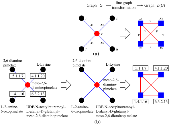
In Fig. 1(a), we consider a graph $G$ and we apply the line graph transformation over this graph $G$. The result of this transformation is the line graph of $G$, $L(G)$. We see that, under the line graph transformation, the nodes of $L(G)$ are the edges of $G$, with two nodes of $L(G)$ adjacent whenever the corresponding edges of $G$ are. If $x=(u,v)$ is an edge of $G$, then the degree of $x$ (deg $(x)$) (i.e., number of edges connected to the node $x$) in $L(G)$ can be written as: deg $(u)$ + deg $(v)$ - 2. The example shown in Fig. 1(a) can correspond to a synthetic network generated by the BA model, where the network is only composed by one kind of nodes. In this case, the edges of the initial network $E(G)$ do not correspond to any physical entity. The line graph transformation becomes more meaningful when those edges $E(G)$ have physical meaning.

This concept of line graph transformation has similarities to the representation of metabolic networks as we can see in Fig. 1(b). Fig. 1(b) (left) shows a real subgraph from the Lysine Biosynthesis metabolic network in the ordinary representation of biochemical pathways. We see that the nodes are chemical compounds and edges are represented by chemical reactions . In this example, nodes and edges have physical meaning. There are five chemical compounds and four chemical reactions in that representation. ¿From this representation we can construct the graph $G$ which only contains compounds as nodes (chemical compound network). Two nodes are linked by an edge when they occur (either as substrates or products) in the same chemical reaction. After applying the line graph transformation on the graph $G$, we obtain the graph $L(G)$ which only contains reactions as nodes (reaction network). The graph $G$ (compound network) will have a degree distribution $P_{G}(k)$, and the graph $L(G)$ (reaction network), obtained through the line graph transformation, will allow us to study its degree distribution $P_{L(G)}(k)$ (or other topological observable). In particular, we focus on the correlation between both degree distributions $P_{G}(k)$ and $P_{L(G)}(k)$, through the line graph transformation. In these figures, we see clearly the close relationship between the line graph transformation and real metabolic networks illustrating the motivation of our analysis. In this example, the line graph transformation becomes more meaningful.

However, we must notice that in some cases the line graph transformation could give rise to spurious nodes. To be concrete, we will use the terminology of chemical compounds/reactions, but this explanation can be extended to any other similar graph structure. These spurious nodes appear when the reactions have more than one product (or substrate) as chemical compounds. When these cases appear, the compound graph $G$ generated (as explained later with Fig. 6) will have extra edges, and consequently the line graph transformation will generate reactions as nodes which do not exist in the real metabolic process. We have analysed this issue and a detailed explanation for the case of metabolic networks can be found in Sec. III.

Figure 1: (a) Graph $G$ is an initial network. $L(G)$ is the corresponding line graph network. (b) A representation of one subgraph from the Lysine Biosynthesis metabolic network. The graph $G$ only contains compounds as nodes (chemical compound network). Two compounds are linked by an edge when they occur in the same chemical reaction. Applying the line graph transformation we generate the line graph $L(G)$, which is the chemical reaction graph embedded in the metabolic network, where the nodes are the reactions. This example illustrates the close relationship between the line graph transformation and the metabolic network.

The main feature underlying the line graph transformation can be summarized as follows: We assume that the initial network has the scale-free topology as $P(k)\approx k^{-\gamma}$. As the degree of each transformed node (i.e., an edge in $G$) will be roughly around $k$, the distribution of the line graph $L(G)$ should be $k\cdot k^{-\gamma}$ = $k^{-\gamma+1}$ with degree around $k$. Therefore, we can conclude that if we have a graph $G$ with a probability distribution following a power-law as $k^{-\gamma}$, then $L(G)$ will follow a power-law as $k^{-\gamma+1}$. We have developed two models to reproduce the behavior of the line graph transformation over the scale-free network. In the first one we solve the discrete equation for the degree distribution of the line graph and in the second one we use the inverted beta distribution. A detailed mathematical explanation on these models can be found in the next subsections.

Figure 2: Eq. (3) is numerically computed with the BA model by fixing degree $j=j_{0}$ ($j_{0}=10,20,50$). 30 trials of BA networks of 10000 nodes are computed for each $j_{0}$ in order to have enough statistics. The results reproduce Eq. (4) with $\gamma^{\prime}=-2$ (continuous lines).

2.2 Discrete equation for the degree distribution of a transformed graph

We asumme the following: $A)$ degree distribution of an original scale-free network follows $|\{v|deg(v)=d\}|\propto d^{-\gamma}$ if $(d>m_{0})$, and $|\{v|deg(v)=d\}|=0$ otherwise. $B)$ edges are randomly generated under $(A)$. Precisely, $deg(u)$ is independent of $deg(v)$ for each edge $(u,v)$. Hence, if $deg(u)$ is $1+d_{1}$ and $deg(v)$ is $1+d_{2}$, the transformed node corresponding to edge $(u,v)$ has degree $d_{1}+d_{2}$. The following relations hold from $(A)$ and $(B)$: $Prob\,[deg(v)=1+d_{i}]\propto\,\,\,(1+d_{i})^{-\gamma}$ with $i$=1,2, for a randomly generated edge ($u$, $v$), where $d_{1}+1$, $d_{2}+1$ $\geq$ $m_{0}$. Therefore, degree distribution of a transformed node would be given by:

$$Prob\,[deg{(u,v)}=d]\propto\sum_{d=d_{1}+d_{2}\atop{d_{1}+1\geq m_{0}\atop{d_{2}+1\geq m_{0}}}}(1+d_{1})^{-\gamma+1}\cdot(1+d_{2})^{-\gamma+1}.$$ (1)

This equation can be expressed as:

$$Prob\,[deg{(u,v)}=d]\propto\sum_{x=m_{0}}^{d_{0}-m_{0}}[{x^{1-\gamma}\cdot(d_{0}-x)^{1-\gamma}}]$$ (2)

with $d_{0}$ = $d+2$ and $x=1+d_{1}$. We are also able to sum in a discrete way in terms of polygamma functions (see the next subsection).

Though we have assumed that $deg(u)$ is independent from $deg(v)$, this assumption can be weakened to the condition that the original network shows no assortative mixing (neutral network). By assortative (disassortative) mixing in networks we understand the preference for nodes with high degree to connect to other high (low) degree nodes [20, 21]. We could choose randomly one edge and we consider the node reached by following that edge. Following Newman [20], the degree distribution for the node at the end of a randomly chosen edge will be: $(k+1)\cdot P(k+1)$, if we only consider the number of edges leaving the node (i.e., not taking into account the node we arrived along). Therefore, the probability distribution $e_{jk}$ of all edges ($u$,$v$) that link together nodes with degree $j+k$ (sum of the degrees of the nodes at the ends of $(u,v)$ edge) would be approximated as:

$$e_{jk}\propto(j+1)\cdot(j+1)^{-\gamma}(k+1)\cdot(k+1)^{-\gamma}.$$ (3)

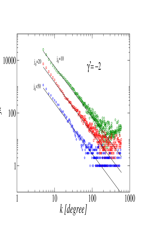
In order to validate Eq. (3) with the BA model, we compute $e_{jk}$ by using several fixed values of $j=j_{0}$. By fixing $j$, Eq. (3) can be written as:

$$e_{{j_{0}k}}\propto C(j_{0})\cdot(k+1)^{-\gamma+1},$$ (4)

where $C(j_{0})$ is a constant, and as $\gamma=3$ for the BA model, $\gamma^{\prime}=-\gamma+1$ should be $-2$. We show the results of our numerical computation in Fig. 2. We see three power-law with exponent $\gamma^{\prime}=-2$ for three different values of $j_{0}$. These results indicate that Eq. (3) is a valid expression for the BA model. It is worth noticing that $e_{jk}=e_{kj}$.

Figure 3: Analysis with synthetic network. (a) Circles (blue): degree distribution generated by using the Barabasi-Albert model [3, 10] with $m_{0}$=$m$=5 (in what follows, $m_{0}$=$m$). The synthetic network follows the power-law distribution $P(k)\approx k^{-\gamma}$ with exponent $\gamma$ = $2.9\pm 0.1$ (continuous line). Diamonds (red): the distribution of the transformed scale-free network also follows a power-law with exponent $\gamma$= $1.9\pm 0.1$ (dashed line). We took average of 10 BA networks of 10000 nodes.(b) Inverted beta distribution (continuous line) with parameters $\beta=17$, $\alpha=1$ and $a=m_{0}=5$ and polygamma distribution for $\gamma=3$ (dash-dotted line). In the inset we show the transformed network data together the polygamma distribution in linear-linear scale. It is interesting to note that the peak found in the transformed network does not exist in the original network. This feature can also be predicted by our theoretical model.

In order to compare with Eq. (1), we sum for all the possible degrees of the two vertices at either end of edges ($u$,$v$) which can generate transformed nodes with degree $d$:

$$Prob\,[deg{(u,v)}=d]=\sum_{d=j+k\atop{j+1\geq m_{0}\atop{k+1\geq m_{0}}}}e_{jk}\propto\sum_{d=j+k\atop{j+1\geq m_{0}\atop{k+1\geq m_{0}}}}(j+1)^{-\gamma+1}\cdot(k+1)^{-\gamma+1},$$ (5)

and Eq. (1) holds.

Although in [20] it is suggested that the BA model is not assortative (neutral scale-free network) (i.e., Pearson correlation function gives a zero result), Redner and Krapivsky [22] pointed out that obvious degree correlations exist in BA model (older nodes tend to be connected) and in similar growth models. However, as we have seen in Fig. 2, Eq. (3) is a good approximation for the BA model.

2.3 Analysis in terms of Polygamma functions

The digamma function is defined as: $\Psi(z)=\frac{d}{dz}\ln\Gamma(z)=\frac{\Gamma^{\prime}(z)}{\Gamma(z)}$ where $\Gamma(z)$ is an extension of the factorial to complex and real numbers and it is analytic everywhere except at $z=0,-1,-2,-3...$. The $n$th derivate of $\Psi$ is named the Polygamma function, denoted $\psi_{n}(z)$. The notation $\psi_{0}(z)$ is frequently used for the digamma function itself as $\psi_{n}(z)=\frac{d^{n}}{dz^{n}}\frac{\Gamma^{\prime}(z)}{\Gamma(z)}=\frac{d^{n}}{dz^{n}}\psi_{0}(z)$. Other useful identities are

$$\frac{d\psi_{0}}{dz}=\sum_{k=0}^{\infty}\frac{1}{(z+k)^{2}}$$ (6)

and

$$\psi_{0}(x)=-\gamma+\sum_{k=1}^{x-1}\frac{1}{k}$$ (7)

where $\gamma$ is the Euler-Mascheroni constant and $x$ is a positive integer value.

By decomposing Eq. (2) in partial fractions, and by using the polygamma relationships shown above, we can find the expressions for Eq. (2) evaluated with $\gamma=2$ and $\gamma=3$. We detail the calculation for $\gamma=2$. The summation of Eq. (2) can be decomposed in two terms:

$$\sum_{x=m_{0}}^{d_{0}-m_{0}}\frac{A}{x}+\frac{B}{d_{0}-x}$$ (8)

where $A=B=1/d_{0}$.

The first term of the sum gives:

$$\sum_{x=m_{0}}^{d_{0}-m_{0}}\frac{1}{x}=\frac{1}{m_{0}}+\frac{1}{m_{0}+1}+...+\frac{1}{d_{0}-m_{0}+1}+\frac{1}{d_{0}-m_{0}}$$ (9)

and by using Eq. (7), we can write it as: $\psi_{0}(x+1)-\psi_{0}(m_{0})$, with $x=d_{0}-m_{0}$. Analogously, the second term gives the same contribution. Therefore for $\gamma=2$, Eq. (2) reads as:

$$Prob\,[deg{(u,v)}=d]_{\gamma=2}\propto\frac{2}{d_{0}}[\psi_{0}(x+1)-\psi_{0}(m_{0})].$$ (10)

For $\gamma=3$ we have

$$Prob\,[deg{(u,v)}=d]_{\gamma=3}\propto\frac{2}{d_{0}\,^{3}}[\psi_{0}]+\frac{1}{d_{0}\,^{2}}[\psi_{1}]$$ (11)

with

$$\psi_{0}=2[\psi_{0}(x+1)-\psi_{0}(m_{0})]$$ (12)

and

$$\psi_{1}=2[\psi_{1}(m_{0})-\psi_{1}(x+1)],$$ (13)

where $d_{0}=d+2$ and $x=d_{0}-m_{0}$ are integer values.

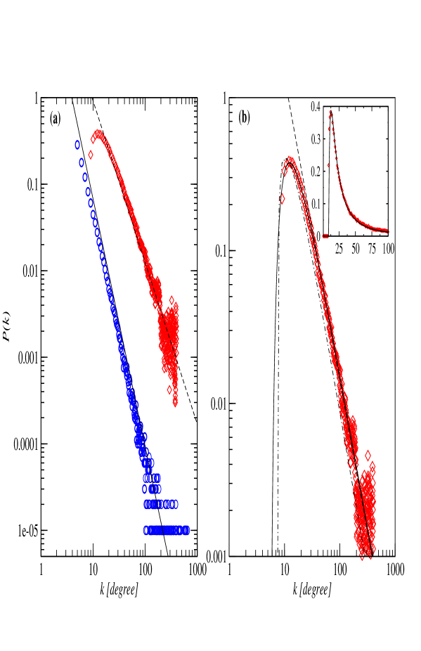
It is interesting to note that $Prob\,[deg{(u,v)}=d]_{\gamma=2}\approx d^{-1}$ and $Prob\,[deg{(u,v)}=d]_{\gamma=3}\approx d^{-2}$ for large $d$, which matches the distribution of $k^{-\gamma+1}$ as we can see in Fig. 3(b).

2.4 Inverted beta distribution

One drawback of the previous approach is that the exponent $\gamma$ is considered as an integer number which constrains its range of quantitative applicability. Hence, we have looked for a continuous function in terms of the exponent $\gamma$. In that sense, we have found that the inverted beta distribution $B(y)\propto{(y-a)^{\beta-1}}/{(1+y-a)^{\alpha+\beta}}$, which is obtained doing the transformation $Y=\frac{1-X}{X}$ over the beta distribution followed by a translation $y\rightarrow\ y-a$, fits well our requirements and it was used successfully to reproduce the data. In addition, it is interesting to note that the distribution shows a power-law tail for large $y$ as: $B(y)\rightarrow{y^{-\alpha-1}}$.

2.5 Theoretical results

Once the theoretical approaches have been introduced, we generate a synthetic scale-free network with exponent $\gamma=2.9$ using the BA model [3, 10] and we study the behavior of the line graph transformation over that scale-free network. We compare the transformed network with the results from the theoretical functions introduced in the previous sections. In Fig. 3(a) we see that the transformed network (diamonds) follows a power-law with exponent $\gamma=1.9$. It is interesting to note that the exponent of this scale-free is exactly reduced by one unit (from the original scale-free network to the transformed network) as it was predicted in the previous sections. As a second result, a peak was found for low degree nodes in the line graph transformed network, indicating that the power-law is like a tail (or asymptotic behaviour) of a more general distribution. In Fig. 3(b) we plot the inverted beta distribution and the polygamma function to compare with the transformed network. We see that the curves reproduce well the peak of the data for low degree $k$ and also shows a power-law tail for higher degree $k$. Both agreements give us confidence about the fairness of both approaches used to study the data.

3 Experimental data

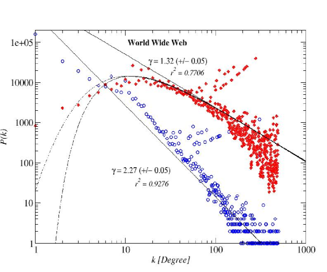
There are several examples, in biological and non-biological networks, which appear to support our theoretical analysis. We have tested our results in the World Wide Web network with a size of 325729 nodes representing web pages being connected by links each other. The dataset was obtained from the website of Notre-Dame Research Group [23]. We must notice that we have considered the links as undirected edges in order to compare with our theoretical approach. In that sense the value of $\gamma$ obtained here could be considered as an average of the $\gamma_{in}$, $\gamma_{out}$ [19]. We have also analysed the protein-protein interaction network for the yeast S. Cerevisae which contains around 1870 proteins as nodes linked by 2240 bidirectional interactions [9, 23]. In Fig. 4 and Fig. 5 we show the data for the WWW network and the protein-protein interaction network respectively. We see that both networks (circles) are following the power-law $P(k)\sim k^{-\gamma}$. In the same figures, we present our results for the corresponding transformed network (diamonds). In both cases, we see that the scale-free topology is preserved and the exponent $\gamma$ is decreased by almost one unit as we expected.

Figure 4: Circles (blue): degree distribution for the WWW network generated with data from [23]. The WWW network follows a power-law with exponent $\gamma=2.27$. Diamonds (red): the distribution of the transformed network also shows a power-law tail with exponent $\gamma=1.32$. We show the inverted beta distribution evaluated with $a=m_{0}=1$ (dashed line), $a=m_{0}=0$ (dash-dotted line), and the beta parameters are $\beta=16$, $\alpha=0.4$. The correlation coefficient is $r^{2}$.

Figure 5: Circles (blue): degree distribution for the protein-protein interaction network S. Cerevisae generated with data from [23]. The protein-protein interaction network follows a power-law with exponent $\gamma=2.20$. Diamonds (red): the distribution of the transformed network also shows a power-law tail with exponent $\gamma=1.32$. We show the inverted beta distribution evaluated with $a=m_{0}=1$ (dashed line), $a=m_{0}=0$ (dash-dotted line), and the beta parameters are $\beta=6$, $\alpha=0.4$. The correlation coefficient is $r^{2}$.

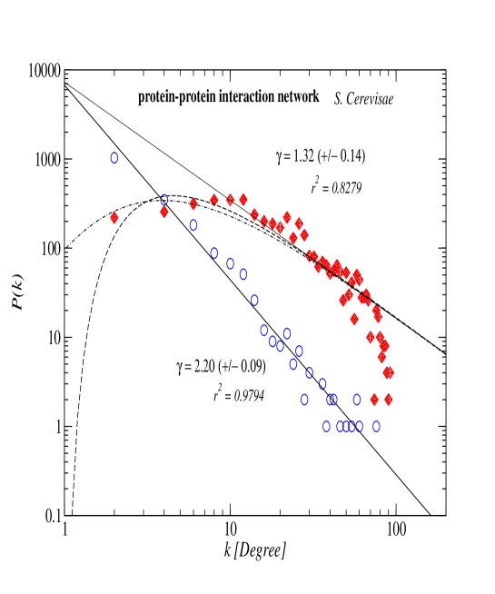
Following with our analysis of real networks, we analyse now the metabolic network from the KEGG database [24] which contained around 10400 chemical compounds and 4100 chemical reactions. The KEGG database is one of the best sites for biochemistry, metabolism, and molecular biology information. As we showed in Fig. 1, the line graph transformation is closely related to the representation of metabolic networks, however we must point out some differences which we have found in our study.

Figure 6: Sketch of metabolic networks. We show two reactions ($R1$, $R2$), with only one common substrate (product) $C4$. The substrate graph $G$ (compounds) is shown with dark blue circles. The reaction graph $L_{real}(G)$ (reactions) is shown with light red circles. To obtain this graph $L_{real}(G)$ we apply a ${\it physical}$ line graph transformation, i.e., we do not transform all the edges from the initial graph and we only generate the same number of nodes in the transformed network as the number of reactions in the real metabolic process. An ordinary line graph transformation would generate nine reactions as nodes in the line graph $L(G)$, when only two reactions exist in the real network.

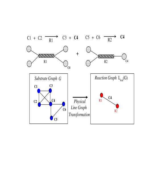
As it is depicted in Fig. 6, in the metabolic networks exist some cases where not all the edges associated to the substrate network should be transformed by the line graph transformation. The main issue is that for each chemical reaction with more than one product (or substrate), we must only transform the same number of edges from the substrate graph as the number of reactions in the real metabolic process. In the case shown in Fig. 6, the resulting network (reaction network), after an ordinary line graph transformation, would generate up to nine nodes (reactions), but only two exist in the real metabolic process. These spurious nodes only appear when one (or some) reaction(s) in the network have more than one product (or substrate). These cases should be transformed as it is shown in Fig. 6 (i.e., by creating only as many nodes in the transformed network as reactions in the real metabolic process). This procedure is called ${physical}$ line graph transformation. The graph generated by the ${physical}$ line graph transformation is denoted by $L_{real}(G)$. In a network where the are some spurious cases as exposed above, we proceed by applying the $physical$ line transformation for these ones, and the ordinary line graph transformation for the rest of the cases. The resulting distribution could be different if we compare it with the distribution generated only by the line graph transformation $P(k)$ $\simeq$ $k^{-\gamma+1}$. The distortion could be larger if there are many of these spurious cases in a network.

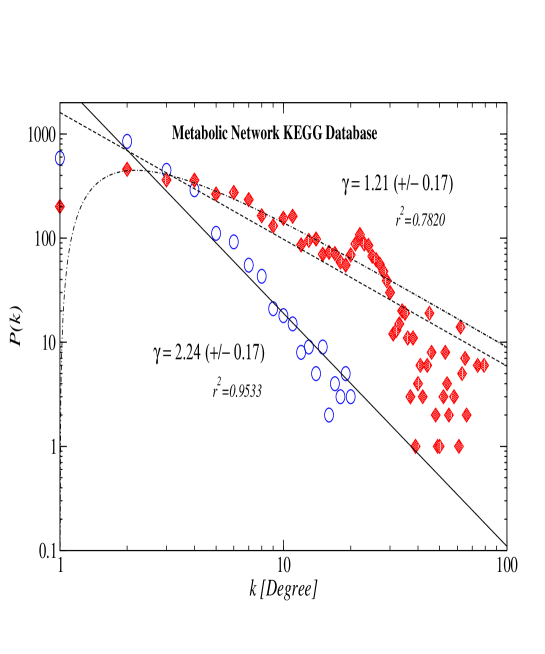
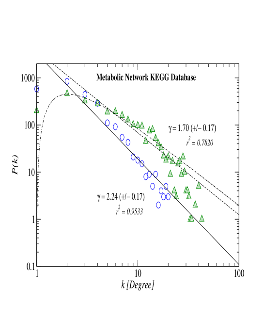
In Fig. 7 we show the degree distribution of the chemical compounds (circles) in the metabolic network from the KEGG database. In the same figure, we have plotted the distribution (diamonds) for the transformed network which corresponds to the reaction network. We see that both distributions follow a power-law and the difference between their exponents is one. However, that transformed network $L(G)$ would not have a full physical meaning because it could have extra reactions as nodes which do not exist in the real metabolic process, as we explained in Fig. 6. In Fig. 8 we plot the transformed network after applying the line graph transformation and the $physical$ line graph transformation for the spurious cases. We see that both graphs are scale-free networks, but in this case, the difference between the exponents is smaller than one, due to the distortion mentioned above.

Experimental results shown in our paper suggest that exponents of the transformed scale-free network may change due to the effect of the spurious cases. However, the experiments also indicate that the scale-free topology is preserved. In particular, if the average number of substrates and products per reaction is small, the spurious cases may not strongly affect, and the scale-free power-law distribution would be preserved.

Figure 7: Circles (blue): Degree distribution for the metabolic networks of KEGG database [24]. The data included the following 9 metabolic pathways: Carbohydrate Metabolism, Energy Metabolism, Lipid Metabolism, Nucleotide Metabolism, Amino Acid Metabolism, Metabolism of Other Amino Acids, Metabolism of Complex Lipids, Metabolism of Complex Carbohydrates and Metabolism of Cofactors and Vitamins. Diamonds (red): The metabolic network follows a power-law with exponent $\gamma=2.24$ (continuous line). Diamonds (red): the transformed distribution of the scale-free network shows a power-law tail with exponent $\gamma=1.21$ (dashed line). With dash-dotted line, we show the inverted beta distribution with parameters $\beta=2.5$, $\alpha=0.25$ evaluated with $a=m_{0}=1$. The correlation coefficient is $r^{2}$.

Figure 8: Circles (blue): Same as Fig. 5. Triangles (green): the distribution of the transformed network after applying the line graph transformation and the $physical$ line graph transformation for the spurious cases. It shows a power-tail with exponent $\gamma=1.70$ (dashed line). With dash-dotted line, we show the inverted beta distribution with parameters $\beta=2.7$, $\alpha=0.7$ evaluated with $a=m_{0}=1$. The correlation coefficient is $r^{2}$.

It is interesting to quote a previous work [25], which analysed the distribution of metabolite connectivities in both substrate and reaction graphs. Although in that paper they do not mention about the line graph transformation technique and, consequently, they do not discuss about the reason of the modification of exponent $\gamma$, they notice that the degree distribution in the reaction graph does not follow a simple power-law and it appears to be governed by two quantitatively different regimes.

4 Conclusions

We have reported on the two complementary representations of a scale-free network using the line graph transformation. This transformation is useful when it is applied on networks where the edges have physical meaning. In particular, we have illustrated that the line graph transformation is closely related to the representation of metabolic network. In this network by using the line graph transformation, the reaction network can be generated and it allows us to study its degree distribution $P(k)$ and other topological observables as clustering degree, for example.

The two goals of the present work can be summarized as follows: We have described the real networks as two complementary representations of a scale-free network, where the second one emerges when the line graph transformation is done over the first one. Our second goal is that we have found that the exponent $\gamma$ is always one unit less than the initial exponent $\gamma$ coming from the original scale-free network. We have seen that the difference of one unit in the exponents of the degree distributions can be found in biological and non-biological networks. We have also carried out a theoretical study of the general distribution underlying the line graph transformation, being successfully to reproduce the tail of the power-law and the peak found for low-degree nodes. However, we should bear in mind that in some particular cases (e.g., metabolic networks) an ordinary line graph transformation applied over a real network could generate extra nodes in the transformed network without a real correspondence. These spurious cases make that the difference between the exponents $\gamma$ could differ from one unit.

We also took advantage of the fact that the BA model is not assortative [20] to compare our results for the discrete equation of a transformed graph. As a future work, an extension of this analysis to assortative networks should be done.

This study is an interesting step forward to understanding large complex networks from this complementary scale-free perspective.

Acknowledgements

This work was partially supported by Grant-in-Aid for Scientific Research on Priority Areas (C) “Genome Information Science” from MEXT. We also thank the Research Group of Notre Dame University for making its database publicly available for research purposes.

References

- [1] P. Erdös, P., A. Rényi, Publ. Math. Inst. Hung. Acad. Sci. 5, 17 (1960).
- [2] B. Bollobás, Random Graphs (Academic Press, London, 1985).
- [3] A.-L. Barabási, R. Albert, Science 286, 509 (1999).
- [4] D.J. Watts, S.H. Strogatz, Nature 393, 440 (1998).
- [5] S. Milgram, Physchol. Today 2, 60 (1967).
- [6] M. Kochen, (ed.) The small world (Ablex, Norwood, NJ, 1989).
- [7] J. Guare, Six Degrees of Separation: A Play (Vintage Books, New York, 1990).
- [8] H. Jeong, B. Tombor, R. Albert, Z.N. Oltvai, A.-L. Barabási, Nature 407, 651 (2000).
- [9] H. Jeong, S.P. Mason, A.-L. Barabási, Z.N. Oltvai, Nature 411, 41 (2001).
- [10] A.-L. Barabási, R. Albert, H. Jeong, Physica A 272, 173 (1999).
- [11] R. Albert, A.-L. Barabási, Phys. Rev. Lett 85, 5234 (2000).
- [12] G. Bianconi, A.-L. Barabási, Europhysics Letters 54 (4), 436 (2001).
- [13] S. N. Dorogovtsev, J. F. F. Mendes, Phys. Rev. E 62, 1842 (2000).
- [14] L. A. N. Amaral, A. Scala, M. Barthelemy, H. E. Stanley, Proc. Natl. Acad. Sci. USA 97, 11149 (2000).
- [15] J.B. Pereira-Leal, A.J. Enright, and C.A. Ouzounis, Proteins 54, 49 (2004).
- [16] A.J. Enright, S. Van Dongen, and C.A. Ouzounis, Nucleic Acids Res. 30, 1575 (2002).
- [17] R. L. Hemminger, L. W. Beineke, Selected Topics in Graph Theory I (Academic Press, London, 1978).
- [18] K. Tipton, S. Boyce, Bioinformatics 16, 34 (2000).
- [19] R. Albert, and A.-L. Barabási, Review of Modern Physics 74, 47 (2002).
- [20] M. E. J. Newman, Phys. Rev. Lett. 89, 208701 (2002).
- [21] M. E. J. Newman, Phys. Rev. E. 67 026126 (2003).
- [22] P. L. Krapivsky and S. Redner, Phys. Review E. 63, 066123 (2003).
- [23] http://www.nd.edu/ networks/database/index.html (2003).
- [24] M. Kanehisa, S. Goto, S. Kawashima, A. Nakaya, Nucleic Acids Res. 30, 42 (2002).
- [25] A. Wagner, D. A. Fell, Proc. R. Soc. London B 268, 1803 (2001).