Electron-acoustic plasma waves:
oblique modulation and envelope solitons

Abstract

Theoretical and numerical studies are presented of the amplitude modulation of electron-acoustic waves (EAWs) propagating in space plasmas whose constituents are inertial cold electrons, Boltzmann distributed hot electrons and stationary ions. Perturbations oblique to the carrier EAW propagation direction have been considered. The stability analysis, based on a nonlinear Schrödinger equation (NLSE), reveals that the EAW may become unstable; the stability criteria depend on the angle $\theta$ between the modulation and propagation directions. Different types of localized EA excitations are shown to exist.

I Introduction

Electron acoustic waves (EAWs) are high-frequency (in comparison with the ion plasma frequency) electrostatic modes STB in plasmas where a ‘minority’ of inertial cold electrons oscillate against a dominant thermalized background of inertialess hot electrons providing the necessary restoring force. The phase speed $v_{ph}$ of the EAW is much larger than the thermal speeds of cold electrons ($v_{th,c}$) and ions ($v_{th,i}$), but is much smaller than the thermal speed of the hot electron component ($v_{th,h}$); $v_{th,\alpha}=(T_{\alpha}/m_{\alpha})^{1/2}$, where $\alpha=c,h,i$ ($m_{\alpha}$ denotes the mass of the component $\alpha$; the Boltzmann constant $k_{B}$ is understood to precede the temperature $T_{\alpha}$ everywhere). Thus, the ions may be regarded as a constant positive charge density background, providing charge neutrality. The EAW frequency is typically well below the cold electron plasma frequency, since the wavelength is larger than the Debye length $\lambda_{h}=(T_{h}/4\pi n_{h0}e^{2})^{1/2}$ involving hot electrons ($n_{\alpha}$ denotes the particle density of the component $\alpha$ everywhere).

The linear properties of the EA waves are well understood [2–5]. Of particular importance is the fact that the EAW propagation is only possible within a restricted range of the parameter values, since both long and short wavelength EAWs are subject to strong Landau damping due to resonance with either the hot or the cold (respectively) electron component. In general, the EAW group velocity scales as $v_{ph}=v_{th,h}\,\sqrt{n_{c}/n_{h}}$; therefore, the condition $v_{th,c}\ll v_{ph}\ll v_{th,h}$ immediately leads to a stability criterion in the form: $T_{c}/T_{h}\ll\sqrt{n_{c}/n_{h}}\ll 1$. A more rigorous investigation [4] reveals that EAWs will be heavily damped, unless the following (approximate) conditions are satisfied: $T_{h}/T_{c}\gtrsim 10$ and $0.2\lesssim n_{c}/n_{e}\lesssim 0.8$ (where $n_{e}=n_{c}+n_{h}$). Even then, however, only wavenumbers $k$ between, roughly, $0.2\,k_{D,c}$ and $0.6\,k_{D,c}$ (for $T_{h}/T_{c}=100$; see in Ref. 4b), will remain weakly damped [$k_{D,c}=(4\pi n_{c,0}e^{2}/T_{c})^{1/2}\equiv\lambda_{D,c}^{-1}$ obviously denotes the cold electron Debye wavenumber]. The stable wavenumber value range is in principle somewhat extended with growing temperature ratio $T_{h}/T_{c}$; see the exhaustive discussion in Refs. 4 and 5.

As far as the nonlinear aspects of EAW are concerned, the formation of coherent EA structures has been considered in a one-dimensional model involving cold Dubouloz ; singh or finite temperature Mace2 ions. Furthermore, such non-envelope solitary structures, associated with a localized compression of the cold electron density, have been shown to exist in a magnetized plasma [9 – 11]. It is worth noting that such studies are recently encouraged by the observation of moving EAW-related structures, reported by spacecraft missions e.g. the FAST at the auroral region [12 – 14], as well as the GEOTAIL and POLAR earlier missions in the magnetosphere [15 – 17]. However, although most solitary wave structures observed are positive potential waves (consistent with an electron hole image), there have also been some negative potential and low velocity structure observations, suggesting that some other type of solitary waves may be present in the magnetosphere [17, 18]. These structures are now believed to be related to EA envelope solitary waves, for instance due to trapping and modulation by ion acoustic density perturbations Dubouloz ; shukla .

Amplitude modulation is a long-known generic feature of nonlinear wave propagation, resulting in higher harmonic generation due to nonlinear self-interactions of the carrier wave in the background medium. The standard method for studying this mechanism is a multiple space and time scale technique redpert ; redpert2 , which leads to a nonlinear Schrödinger equation (NLSE) describing the evolution of the wave envelope. Under certain conditions, it has been shown that waves may develop a Benjamin-Feir-type (modulational) instability (MI), i.e. their modulated envelope may be unstable to external perturbations. Furthermore, the NLSE-based analysis, encountered in a variety of physical systems [21 – 23], reveals the possibility of the existence of localized structures (envelope solitary waves) due to the balance between the wave dispersion and nonlinearities. This approach has long been considered with respect to electrostatic plasma waves [20, 24 – 30].

In this paper, we study the occurrence of modulational instability as well as the existence of envelope solitary structures involving EAWs that propagate in an unmagnetized plasma composed of three distinct particle populations: a population of ‘cold’ inertial electrons (mass $m_{e}$, charge $-e$), surrounded by an environment of ‘hot’ (thermalized Boltzmann) electrons, moving against a fixed background of ions (mass $m_{i}$, charge $q_{i}=+Z_{i}e$), which provide charge neutrality. These three plasma species will henceforth be denoted by $c,\,h$ and $i$, respectively. By employing the reductive perturbation method and accounting for harmonic generation nonlinearities, we derive a cubic Schrödinger equation for the modulated EA wave packet. It is found that the EAWs are unstable against oblique modulations. Conditions under which the modulational instability occurs are given. Possible stationary solutions of the nonlinear Schrödinger equation are also presented.

II The model equations

Let us consider the hydrodynamic–Poisson system of equations for the EAWs in an unmagnetized plasma. The number density $n_{c}$ of cold electrons is governed by the continuity equation

$$\frac{\partial n_{c}}{dt}+\nabla\cdot(n_{c}\,\mathbf{u}_{c})=0\,,$$ (1)

where the mean velocity $\mathbf{u}_{c}$ obeys

$$\frac{\partial\mathbf{u}_{c}}{dt}+\mathbf{u}_{c}\cdot\nabla\mathbf{u}_{c}\,=\,\frac{e}{m_{e}}\,\nabla\,\Phi\,.$$ (2)

Here, the wave potential $\Phi$ is obtained from Poisson’s equation

$$\nabla^{2}\Phi\,=\,-4\pi\,\sum q_{s}\,n_{s}\,=\,4\pi\,e\,(n_{c}\,+n_{h}\,-Z_{i}\,n_{i})\,.$$ (3)

We assume immobile ions ($n_{i}=n_{i,0}$ = constant) and a Boltzmann distribution for the hot electrons, i.e. $n_{h}\approx n_{h,0}\,\exp(e\Phi/k_{B}T_{h})\,$ ($T_{h}$ is electron temperature, $k_{B}$ is the Boltzmann constant), since the EAW frequency is much higher than the ion plasma frequency, and the EA wave phase velocity is much lower than the electron thermal speed $(T_{h}/m_{e})^{1/2}$. The overall quasi-neutrality condition reads

$$n_{c,0}\,+n_{h,0}\,-Z_{i}\,n_{i,0}\,=\,0\,.$$ (4)

Re-scaling all variables and developing around $\Phi=0$, Eqs. (1) - (3) can be cast in the reduced form

$$\frac{\partial n}{dt}+\nabla\cdot(n\,\mathbf{u}) = 0\,,$$

$$\frac{\partial\mathbf{u}}{dt}+\mathbf{u}\cdot\nabla\mathbf{u}\, = \,\nabla\phi\,,$$

and

$$\nabla^{2}\phi\,=\,\phi+\frac{1}{2}\,\phi^{2}+\frac{1}{6}\,\phi^{3}+\,\beta\,(n-1)\,,$$ (5)

where all quantities are non-dimensional: $n=n_{c}/n_{c,0}$, $\mathbf{u}=\mathbf{u}_{c}/v_{0}$ and $\phi=\Phi/\Phi_{0}$; the scaling quantities are, respectively: the equilibrium density $n_{c,0}$, the ‘electron acoustic speed’ $v_{0}=c_{s,h}=(k_{B}T_{h}/m_{e})^{1/2}$ and $\Phi_{0}=(k_{B}T_{h}/e)$. Space and time are scaled over the Debye length $\lambda_{D,h}=(k_{B}T_{h}/4\pi n_{h,0}e^{2})^{1/2}$ and the inverse plasma frequency $\omega_{p,h}^{-1}=\lambda_{D,h}/c_{s}=(4\pi n_{h,0}e^{2}/m_{e})^{-1/2}$, respectively. The dimensionless parameter $\beta$ denotes the ratio of the cold to the hot electron component i.e. $\beta=n_{c}/n_{h}$. Recall that Landau damping in principle prevails on both high and low values of $beta$ (cf. the discussion in the introduction). According to the results of Ref. [4b], for undamped EA wave propagation one should consider: $0.25\lesssim\beta\lesssim 4$.

III Perturbative analysis

Let $S$ be the state (column) vector $(n,\,\mathbf{u},\,\phi)^{T}$, describing the system’s state at a given position $\mathbf{r}$ and instant $t$. Small deviations will be considered from the equilibrium state $S^{(0)}=(1,\,\mathbf{0},\,0)^{T}$ by taking $S=S^{(0)}\,+\,\epsilon\,S^{(1)}+\,\epsilon^{2}\,S^{(2)}+\,...=S^{(0)}\,+\,\,\sum_{n=1}^{\infty}\epsilon^{n}\,S^{(n)}$, where $\epsilon\ll 1$ is a smallness parameter. Following the standard multiple scale (reductive perturbation) technique redpert , we shall consider a set of stretched (slow) space and time variables $\zeta\,=\,\epsilon(x-\lambda\,t)$ and $\tau\,=\,\epsilon^{2}\,t\,,$, where $\lambda$ is to be later determined by compatibility requirements. All perturbed states depend on the fast scales via the phase $\theta_{1}=\mathbf{k\cdot r}-\omega t$ only, while the slow scales only enter the $l-$th harmonic amplitude $S_{l}^{(n)}$, viz. $S^{(n)}\,=\,\sum_{l=-\infty}^{\infty}\,S_{l}^{(n)}(\zeta,\,\tau)\,e^{il(\mathbf{k\cdot r}-\omega t)}$; the reality condition $S_{-l}^{(n)}={S_{l}^{(n)}}^{*}$ is met by all state variables. Two directions are therefore of importance in this (three-dimensional) problem: the (arbitrary) propagation direction and the oblique modulation direction, defining, say, the $x-$axis, characterized by a pitch angle $\theta$. The wave vector $\mathbf{k}$ is thus taken to be $\mathbf{k}=(k_{x},\,k_{y})=(k\,\cos\theta,\,k\,\sin\theta)$.

Substituting the above expressions into the system of equations (5) and isolating distinct orders in $\epsilon$, we obtain the $n$th-order reduced equations

$$-il\omega n_{l}^{(n)}\,+\,il\mathbf{k\cdot u}_{l}^{(n)}\,-\,\lambda\,\frac{\partial n_{l}^{(n-1)}}{\partial\zeta}\,+\,\frac{\partial n_{l}^{(n-2)}}{\partial\tau}$$

$$\,+\,\frac{\partial u_{l,x}^{(n-1)}}{\partial\zeta}$$

$$\,+\,\sum_{n^{\prime}=1}^{\infty}\,\sum_{l^{\prime}=-\infty}^{\infty}\biggl{[}il\mathbf{k\cdot u}_{l-l^{\prime}}^{(n-n^{\prime})}\,n_{l^{\prime}}^{(n^{\prime})}\qquad\qquad\qquad$$

$$+\,\frac{\partial}{\partial\zeta}\biggl{(}n_{l^{\prime}}^{(n^{\prime})}u_{(l-l^{\prime}),x}^{(n-n^{\prime}-1)}\biggr{)}\biggr{]}\,=\,0\,,\quad$$ (6)

$$-il\omega\mathbf{u}_{l}^{(n)}\,-\,il\mathbf{k}\phi_{l}^{(n)}\,-\,\lambda\,\frac{\partial\mathbf{u}_{l}^{(n-1)}}{\partial\zeta}\,+\,\frac{\partial\mathbf{u}_{l}^{(n-2)}}{\partial\tau}$$

$$\,-\,\frac{\partial\phi_{l}^{(n-1)}}{\partial\zeta}\,\hat{x}$$

$$\,+\,\sum_{n^{\prime}=1}^{\infty}\,\sum_{l^{\prime}=-\infty}^{\infty}\biggl{[}il^{\prime}\mathbf{k\cdot u}_{l-l^{\prime}}^{(n-n^{\prime})}\,\mathbf{u}_{l^{\prime}}^{(n^{\prime})}\qquad\qquad\qquad$$

$$+\,u_{(l-l^{\prime}),x}^{(n-n^{\prime}-1)}\,\frac{\partial\mathbf{u}_{l^{\prime}}^{(n^{\prime})}}{\partial\zeta}\biggr{]}\,=\,0\,,$$ (7)

and

$$-(l^{2}k^{2}+1)\,\phi_{l}^{(n)}\,-\,\beta\,n_{l}^{(n)}\qquad\qquad\qquad\qquad\qquad\qquad$$

$$\,+2ilk_{x}\,\frac{\partial\phi_{l}^{(n-1)}}{\partial\zeta}\,+\,\frac{\partial^{2}\phi_{l}^{(n-2)}}{\partial\zeta^{2}}\qquad\qquad\qquad\qquad$$

$$-\,\frac{1}{2}\,\sum_{n^{\prime}=1}^{\infty}\,\sum_{l^{\prime}=-\infty}^{\infty}\,\phi_{l-l^{\prime}}^{(n-n^{\prime})}\,\phi_{l^{\prime}}^{(n^{\prime})}\,\qquad\qquad\qquad\qquad$$

$$-\,\frac{1}{6}\,\sum_{n^{\prime},n^{\prime\prime}=1}^{\infty}\,\sum_{l^{\prime},l^{\prime\prime}=-\infty}^{\infty}\,\phi_{l-l^{\prime}-l^{\prime\prime}}^{(n-n^{\prime}-n^{\prime\prime})}\,\phi_{l^{\prime}}^{(n^{\prime})}\,\phi_{l^{\prime\prime}}^{(n^{\prime\prime})}\,=\,0\,.\quad$$ (8)

For convenience, one may consider instead of the vectorial relation (7) the scalar one obtained by taking its scalar product with the wavenumber $\mathbf{k}$.

The standard perturbation procedure now consists in solving in successive orders $\sim\epsilon^{n}$ and substituting in subsequent orders. For instance, the equations for $n=2$, $l=1$

$$-il\omega n_{l}^{(1)}\,+\,il\mathbf{k\cdot u}_{l}^{(1)}\,=\,0\,,$$ (9)

$$-il\omega\mathbf{u}_{l}^{(1)}\,-\,il\mathbf{k}\phi_{l}^{(1)}\,=\,0$$ (10)

and

$$-(l^{2}k^{2}+1)\,\phi_{l}^{(1)}\,-\,\beta\,n_{l}^{(1)}\,=\,0$$ (11)

provide the familiar EAW dispersion relation

$$\omega^{2}\,=\frac{\beta\,k^{2}}{k^{2}+1}\,,$$ (12)

i.e. restoring dimensions

$$\omega^{2}\, = \omega_{p,c}^{2}\,\frac{k^{2}}{k^{2}+k_{D}^{2}}\,\equiv\,\frac{c_{s,c}^{2}\,k^{2}}{1+k^{2}\,{\lambda_{D}}_{h}^{2}}\,,$$ (13)

where $\omega_{p,c}=c_{s,c}/\lambda_{D,c}=(4\pi n_{c,0}e^{2}/m_{e})^{1/2}$ (associated with the cold component), and determine the first harmonics of the perturbation viz.

$$n_{1}^{(1)}\, = -\,\frac{1+k^{2}}{\beta}\phi_{1}^{(1)}\,,\qquad\mathbf{k\cdot u}_{1}^{(1)}\,=\,\omega\,n_{1}^{(1)}\,$$

$$\qquad u_{1,x}^{(1)}\, = \frac{\omega}{k}\cos\theta\,n_{1}^{(1)}\,\,,\qquad u_{1,y}^{(1)}\,=\frac{\omega}{k}\sin\theta\,n_{1}^{(1)}\,\,.\qquad$$ (14)

Proceeding in the same manner, we obtain the second order quantities, namely the amplitudes of the second harmonics $S_{2}^{(2)}$ and constant (‘direct current’) terms $S_{0}^{(2)}$, as well as a non-vanishing contribution $S_{1}^{(2)}$ to the first harmonics. The lengthy expressions for these quantities, omitted here for brevity, are conveniently expressed in terms of the first-order potential correction $\phi_{1}^{(1)}$. The equations for $n=2$, $l=1$ then provide the compatibility condition: $\lambda\,=v_{g}(k)\,=\frac{\partial\omega}{\partial k_{x}}=\omega^{\prime}(k)\cos\theta=$ $\frac{\omega^{3}}{\beta k^{3}}\,\cos\theta$; $\lambda$ is, therefore, the group velocity in the $x$ direction.

IV Derivation of the Nonlinear Schrödinger Equation

Proceeding to the third order in $\epsilon$ ($n=3$), the equations for $l=1$ yield an explicit compatibility condition in the form of the Nonlinear Schrödinger Equation

$$i\,\frac{\partial\psi}{\partial\tau}+P\,\frac{\partial^{2}\psi}{\partial\zeta^{2}}+Q\,|\psi|^{2}\,\psi=0\,.$$ (15)

where $\psi$ denotes the electric potential correction $\phi_{1}^{(1)}$. The ‘slow’ variables $\{\zeta,\tau\}$ were defined above.

The group dispersion coefficient $P$ is related to the curvature of the dispersion curve as $P\,=\,\frac{1}{2}\,\frac{\partial^{2}\omega}{\partial k_{x}^{2}}\,=\,\frac{1}{2}\,\biggl{[}\omega^{\prime\prime}(k)\,\cos^{2}\theta\,+\omega^{\prime}(k)\,\frac{\sin^{2}\theta}{k}\biggr{]}$; the exact form of P reads

$$P(k)\,=\,\frac{1}{\beta}\frac{1}{2\,\omega}\,\biggl{(}\frac{\omega}{k}\biggr{)}^{4}\,\biggl{[}1-\biggl{(}1+3\,\frac{1}{\beta}\,\omega^{2}\biggr{)}\,\cos^{2}\theta\biggr{]}\,.$$ (16)

The nonlinearity coefficient $Q$ is due to the carrier wave self-interaction in the background plasma. Distinguishing different contributions, $Q$ can be split into three distinct parts, viz. $Q=\,Q_{0}\,+\,Q_{1}\,+\,Q_{2}$, where

$$Q_{0} = \,\frac{\omega^{3}}{2\,\beta^{3}\,k^{2}}\,\frac{1}{(1+\,k^{2})^{3}-\cos^{2}\theta}\,$$ (17)

$$\biggl{\{}(1+\,k^{2})^{4}(1+2\beta+\,k^{2})$$

$$+\biggl{[}\beta^{2}+4\beta(1+\,k^{2})^{3}+4(1+\,k^{2})^{4}(2+\,2k^{2}+\,k^{4})\biggr{]}\,$$

$$\qquad\times\cos^{2}\theta\biggr{\}}\,,$$

$$Q_{1} = \,\frac{\omega^{3}}{4\,\beta\,k^{2}}\,,$$ (18)

$$Q_{2} = \,-\frac{k^{2}}{12\,\omega^{3}}\,\biggl{[}\frac{\omega^{6}}{\beta\,k^{6}}\,+\frac{\omega^{2}}{k^{2}}\,+3\,(3+8\,k^{2})\biggr{]}\,.$$ (19)

We observe that only the first contribution $Q_{0}$, related to self-interaction due to the zeroth harmonics, is angle-dependent, while the latter two - respectively due to the cubic and quadratic terms in (5c) - are isotropic. Also, $Q_{2}$ is negative, while $Q_{0}$, $Q_{1}$ are positive for all values of $k$ and $\beta$. For parallel modulation, i.e. $\theta=0$, the simplified expressions for $\left.P\right|_{\theta=0}$ and $\left.Q\right|_{\theta=0}$ are readily obtained from the above formulae; note that $\left.P\right|_{\theta=0}<0$, while $\left.Q\right|_{\theta=0}$, even though positive for $k\rightarrow 0$ (see below), changes sign at some critical value of $k$.

A preliminary result regarding the behaviour of the coefficients $P$ and $Q$ for long wavelengths may be obtained by considering the limit of small $k\ll 1$ in the above formulae. The parallel ($\theta=0$) and oblique ($\theta\neq 0$) modulation cases have to be distinguished straightaway. For small values of $k$ ($k\ll 1$), $P$ is negative and varies as

$$P\bigr{|}_{\theta=0}\,\approx-\frac{3}{2}\,{\sqrt{\beta}}\,k$$ (20)

in the parallel modulation case (i.e. $\theta=0$), thus tending to zero for vanishing $k$, while for $\theta\neq 0$, $P$ is positive and goes to infinity as

$$P\bigr{|}_{\theta\neq 0}\,\approx\frac{\sqrt{\beta}}{2\,k}\,\sin^{2}\theta$$ (21)

for vanishing $k$. Therefore, the slightest deviation by $\theta$ of the amplitude variation direction with respect to the wave propagation direction results in a change in sign of the group-velocity dispersion coefficient $P$. On the other hand, $Q$ varies as $\sim 1/k$ for small $k\ll 1$. For $\theta\neq 0$, $Q$ is negative

$$Q\bigr{|}_{\theta\neq 0}\,\approx\,-\frac{1}{12\,\beta^{3/2}}\,(3+\beta)^{2}\,\frac{1}{k}\,,$$ (22)

while for vanishing $\theta$, the approximate expression for $Q$ changes sign, i.e.

$$Q\bigr{|}_{\theta=0}\,\approx\,+\frac{1}{12\,\beta^{3/2}}\,(3+\beta)^{2}\,\frac{1}{k}\,.$$ (23)

In conclusion, both $P$ and $Q$ change sign when ‘switching on’ theta. Since the wave’s (linear) stability profile, expected to be influence by obliqueness in modulation, essentially relies on (the sign of) the product $PQ$ (see below), we see that long wavelengths will always be stable.

V Stability analysis

The standard stability analysis [20, 21, 31] consists in linearizing around the monochromatic (Stokes’s wave) solution of the NLSE (15): $\psi\,=\,{\hat{\psi}}\,e^{iQ|\psi|^{2}\tau}\,+\,c.c.\,,$ (notice the amplitude dependence of the frequency) by setting ${\hat{\psi}}\,=\,{\hat{\psi}}_{0}\,+\,\epsilon\,{\hat{\psi}}_{1}\,,$ and taking the perturbation ${\hat{\psi}}_{1}$ to be of the form: ${\hat{\psi}}_{1}\,=\,{\hat{\psi}}_{1,0}\,e^{i({\hat{k}}\zeta-{\hat{\omega}}\tau)}\,+\,c.c.$ (the perturbation wavenumber $\hat{k}$ and the frequency $\hat{\omega}$ should be distinguished from their carrier wave homologue quantities, denoted by $k$ and $\omega$). Substituting into (15), one thus readily obtains the nonlinear dispersion relation

$$\hat{\omega}^{2}\,=\,P^{2}\,\hat{k}^{2}\,\biggl{(}\hat{k}^{2}\,-\,2\frac{Q}{P}|\hat{\psi}_{0}|^{2}\biggr{)}\,.$$ (24)

The wave will obviously be stable if the product $PQ$ is negative. However, for positive $PQ>0$, instability sets in for wavenumbers below a critical value $\hat{k}_{cr}=\sqrt{2\frac{Q}{P}}|\hat{\psi}_{0}|$, i.e. for wavelengths above a threshold: $\lambda_{cr}=2\pi/\hat{k}_{cr}$; defining the instability growth rate $\sigma=|Im\hat{\omega}(\hat{k})|$, we see that it reaches its maximum value for $\hat{k}=\hat{k}_{cr}/\sqrt{2}$, viz.

$$\sigma_{max}=|Im\hat{\omega}|_{\hat{k}=\hat{k}_{cr}/\sqrt{2}}\,=\,|Q|\,|\hat{\psi}_{0}|^{2}\,.$$ (25)

We conclude that the instability condition depends only on the sign of the product $PQ$, which may now be studied numerically, relying on the exact expressions derived above.

In figures 1 to 3, we have depicted the $PQ=0$ boundary curve against the normalized wavenumber $k/k_{D}$ (in abscissa) and angle $\theta$ (between $0$ and $\pi$); the area in black (white) represents the region in the $(k-\theta)$ plane where the product is negative (positive), i.e. where the wave is stable (unstable). For illustration purposes, we have considered w a wide range of values of the wavenumber $k$ (normalized by the Debye wavenumber $k_{D,h}$; nevertheless, recall that the analysis is rigorously valid in a quite restricted region of (low) values of $k$. Modulation angle $\theta$ is allowed to vary between zero and ${\pi}$ (see that all plots are $\frac{\pi}{2}$- periodic).

As analytically predicted above, the product $PQ$ is negative for small $k$, for all values of theta; long wavelengths will always be stable. The product possesses positive values for angle values between zero and $\theta\approx 1$ rad $\approx 57{}^{\circ}$; instability sets in above a wavenumber threshold which, even though unrealistically high for $\theta=0$, is clearly seen to decrease as the modulation pitch angle $\theta$ increases from zero to approximately 30 degrees, and then increases again up to $\theta\approx 57{}^{\circ}$. Nevertheless, beyond that value (and up to $\pi/2$) the wave remains stable; this is even true for the wavenumber regions where the wave would be unstable to a parallel modulation. The inverse effect is also present: even though certain $k$ values correspond to stability for $\theta=0$, the same modes may become unstable when subject to an oblique modulation ($\theta\neq 0$). In all cases, the wave appears to be globally stable to large angle $\theta$ modulation (between 1 and $\pi/2$ radians, i.e. $57{}^{\circ}$ to $90{}^{\circ})$.

It is interesting to trace the influence of the percentage of the cold electron population (related to $\beta=n_{c}/n_{h}$) on the qualitative remarks of the preceding paragraph. For values of $\beta$ below unity, there seems to be only a small effect on the wave’s stability, as described above; cf. figs. 1, 2. As a matter of fact, $\beta<1$ appears to be valid in most reports of satellite observations, carried out at the edges of the Auroral Kilometric Radiation (AKR) region (where the hot and cold electron population co-existence is observed) Berthomier2000 ; obs1 ; obs3 ; furthermore, theoretical studies have suggested that a low $\beta$ value (in addition to a high hot to cold electron temperature ratio) are conditions ensuring EAW stability i.e. resistance to damping Gary ; Berthomier2000 . Nevertheless, notice for rigor that allowing for a high fraction of cold electrons ($\beta\gtrsim 3.5$) leads to a strong modification of the the EA wave’s stability profile, and even produces instability in otherwise stable regions; cf. fig. 3 (where an unrealistic value of $\beta=5$ was considered). In a qualitative manner, adding cold electrons seems to favour stability to quasi-parallel modulation (small $\theta$), yet allows for instability to higher $\theta$ oblique modulation; cf. figs. 1 to 3. Since the black/white regions in the figures correspond to dark/bright type solitons (see below), we qualitatively deduce that a solitary wave of either type may become unstable in case of an important increase in minority electron component, i.e. well above $\beta=1$; see fig. 5. Notice that the critical value of the cold-to-hot electron number ratio $\beta$ in order for such phenomena to occur may be quite low if oblique modulation is considered; see e.g. fig. 5b.

VI Envelope solitary waves

The NLSE (15) is known to possess distinct types of localized constant profile (solitary wave) solutions, depending on the sign of the product $PQ$. Following Ref. Hasegawa ; Fedele , we seek a solution of Eq. (15) in the form $\psi(\zeta,\tau)=\sqrt{\rho(\zeta,\tau)}\,e^{i\,\Theta(\zeta,\tau)}$, where $\rho$, $\sigma$ are real variables which are determined by substituting into the NLSE and separating real and imaginary parts. The different types of solution thus obtained are summarized in the following.

For $PQ>0$ we find the (bright) envelope soliton commentFedele1

$$\rho=\rho_{0}\,sech^{2}\biggl{(}\frac{\zeta-u\,\tau}{L}\biggr{)}\,,\qquad\Theta=\frac{1}{2P}\,\bigl{[}u\,\zeta\,-(\Omega+\frac{1}{2}u^{2})\tau\bigr{]}\,,$$ (26)

representing a bell – shaped localized pulse travelling at a speed $u$ and oscillating at a frequency $\Omega$ (for $u=0$). The pulse width $L$ depends on the (constant) maximum amplitude square $\rho_{0}$ as

$$L=\sqrt{\frac{2P}{Q\,\rho_{0}}}\,.$$ (27)

For $PQ<0$ we have the dark envelope soliton (hole) commentFedele1

$$\rho = \rho_{1}\,\biggl{[}1-\,sech^{2}\biggl{(}\frac{\zeta-u\,\tau}{L^{\prime}}\biggr{)}\biggr{]}\,=\,\rho_{1}\,tanh^{2}\biggl{(}\frac{\zeta-u\,\tau}{L^{\prime}}\biggr{)}\,,$$

$$\Theta = \frac{1}{2P}\,\biggl{[}u\,\zeta\,-\biggl{(}\frac{1}{2}u^{2}-2PQ\rho_{1}\biggr{)}\,\tau\biggr{]}\,,$$ (28)

representing a localized region of negative wave density (shock) travelling at a speed $u$; this cavity traps the electron-wave envelope, whose intensity is now rarefactive i.e. a propagating hole in the center and constant elsewhere. Again, the pulse width depends on the maximum amplitude square $\rho_{1}$ via

$$L^{\prime}=\sqrt{2\biggl{|}\frac{P}{Q\,\rho_{1}}\biggr{|}}\,\qquad.$$ (29)

Finally, looking for velocity-dependent amplitude solutions, for $PQ<0$, one obtains the grey envelope solitary wave Fedele

$$\rho = \rho_{2}\,\biggl{[}1-a^{2}\,sech^{2}\biggl{(}\frac{\zeta-u\,\tau}{L^{\prime\prime}}\biggr{)}\biggr{]}\,,$$

$$\Theta = \frac{1}{2P}\,\biggl{[}V_{0}\,\zeta\,-\biggl{(}\frac{1}{2}V_{0}^{2}-2PQ\rho_{2}\biggr{)}\,\tau+\Theta_{10}\biggr{]}\,$$ (30)

$$\qquad\,-S\,\sin^{-1}\frac{a\,\tanh\bigl{(}\frac{\zeta-u\,\tau}{L^{\prime\prime}}\bigr{)}}{\biggr{[}1-a^{2}\,sech^{2}\biggl{(}\frac{\zeta-u\,\tau}{L^{\prime\prime}}\biggr{)}\biggr{]}^{1/2}}\,,\qquad$$

which also represents a localized region of negative wave density; $\Theta_{10}$ is a constant phase; $S$ denotes the product $S=sign\,P\,\times sign\,(u-V_{0})$. In comparison to the dark soliton (28), note that apart from the maximum amplitude $\rho_{2}$, which is now finite (i.e. non-zero) everywhere, the pulse width of this grey-type excitation

$$L^{\prime\prime}=\sqrt{2\biggl{|}\frac{P}{Q\,\rho_{2}}\biggr{|}}\,\frac{1}{a}$$ (31)

now also depends on $a$, given by

$$a^{2}\,=\,1\,+\,\frac{1}{2PQ}\frac{1}{\rho_{2}}(u^{2}-V_{0}^{2})\,\leq\,1$$ (32)

($PQ<0$), an independent parameter representing the modulation depth ($0<a\leq 1$). $V_{0}$ is an independent real constant which satisfies the condition Fedele

$$V_{0}-\sqrt{2|PQ|\,\rho_{2}}\,\leq\,u\,\leq\,V_{0}+\sqrt{2|PQ|\,\rho_{2}}\quad;$$

for $V_{0}=u$, we have $a=1$ and thus recover the dark soliton presented in the previous paragraph.

Summarizing, we see that the regions depicted in figs. 1 – 3 actually also distinguish the regions where different types of localized solutions may exist: bright (dark or grey) solitons will occur in white (black) regions (the different types of NLS excitations are exhaustively reviewed in Fedele ). Soliton characteristics will depend on dispersion and nonlinearity via the $P$ and $Q$ coefficients; in particular, the sign/absolute value of the ratio $P/Q$ provides, as we saw, the type (bright or dark-grey)/width, respectively, of the localized excitation. Therefore, regions with higher values of $|P/Q|$ will support wider (spatially more extended) localized excitations of either bright or dark/grey type - see fig. 4. Solitons of the latter type (holes) appear to be predominant in the long wavelength region which is of interest here, in agreement with observations, yet may become unstable and give their place to (bright) pulses, in the presence of oblique perturbation (figs. 1, 2) and/or local $n_{c}/n_{h}$- value irregularities (fig. 5). In the short wavelength region, these qualitative results may still be valid, yet quantitatively appear to be rather questionable, since the wave stability cannot be taken for granted due to electron Landau damping. Nevertheless, even so, the EAWs are known to be less heavily damped than Langmuir waves Gary , and may dominate the space plasma (high) frequency spectrum in the presence of different temperature electron populations.

VII Conclusions

This work has been devoted to the study of the modulation of EAWs propagating in an unmagnetized space plasma. Allowing for the modulation to occur in an oblique manner, we have shown that the conditions for the modulational instability depend on the angle between the EAW propagation and modulation directions. In fact, the region of parameter values where instability occurs is rather extended for angle $\theta$ values up to a certain threshold, and, on the contrary, smeared out for higher $\theta$ values (and up to 90 degrees, then going on in a $\frac{\pi}{2}$ - periodic fashion).

Furthermore, we have studied the possibility for the formation of localized structures (envelope EAW solitary waves) in our two electron system. Distinct types of localized excitations (envelope solitons) have been shown to exist. Their type and propagation characteristics depend on the carrier wave wavenumber $k$ and the modulation angle $\theta$. The dominant localized mode at long wavelengths appears to be a rarefactive region of negative wave intensity (hole), which may however become unstable to oblique modulation or variations of the $n_{c}/n_{h}$ ratio. It should be mentioned that both bright and dark/grey envelope excitations are possible within this model; thus, even though the latter appear to be rather privileged within the parameter range where waves are expected not to be heavily damped, the former may exist due to oblique amplitude perturbations. In conclusion, we stress that the qualitative aspects of the observed envelope solitary structures are recovered from our simple fluid model. The present investigation can be readily extended to include the effects of the geomagnetic field, a tenuous electron beam, and on dynamics on the amplitude modulation of the EAWs. The magnetic field effects would produce three-dimensional NLSE in which the longitudinal and transverse (to the external magnetic field direction) group dispersions would be different due to the cold electron polarization effect. The harmonic generation nonlinearities would also be modified by the presence of the external magnetic field.

Figure Captions

Figure 1.

The product $PQ=0$ contour is depicted against the normalized wavenumber $k/k_{D}$ (in abscissa) and angle $\theta$ (between $0$ and $\pi$); black (white) colour represents the region where the product is negative (positive), i.e. the region of linear stability (instability). Furthermore, black (white) regions may support dark (bright)-type solitary excitations. This plot refers to a realistic cold to hot electron ratio equal to $\beta=0.5$ (i.e. one third of the electrons are cold).

Figure 2.

Similar to fig. 1, for $\beta=1$.

Figure 3.

Similar to figures 1, 2 considering a very strong presence of cold electrons ($\beta=5$). Notice the appearance of instability (bright) regions for large angle values and long wavelengths.

Figure 4.

Contours of the ratio $P/Q$ – whose absolute value is related to the square of the soliton width, see (27), (29) – are represented against the normalized wavenumber $k/k_{D,h}$ and angle $\theta$. See that the negative values correspond to two branches (lower half), so that the variation of $P/Q$, for a given wavenumber $k$, does not depend monotonically on $\theta$. $\beta=0.5$ in this plot.

Figure 5.

The $P/Q$ coefficient ratio, whose sign/absolute value is related to the type/width of solitary excitations, is depicted against the cold-to-hot electron density ratio $\beta$. The wavenumber is chosen as $k/k_{D,h}=0.7$. (a) $\theta=0{}^{\circ}$ (parallel modulation): only dark-type excitations exist ($PQ<0$); their width increases with $\beta$. (b) $\theta=60{}^{\circ}$ (oblique modulation): bright/dark excitations exist for $\beta$ below/above $\beta_{cr}\approx 0.8$. The bright/dark soliton width increases/decreases with $\beta$. (c) $\theta=90{}^{\circ}$ (transverse modulation). A rather (unacceptably) high value of $\beta$ was taken, to stress the omnipresence of dark–type excitations.

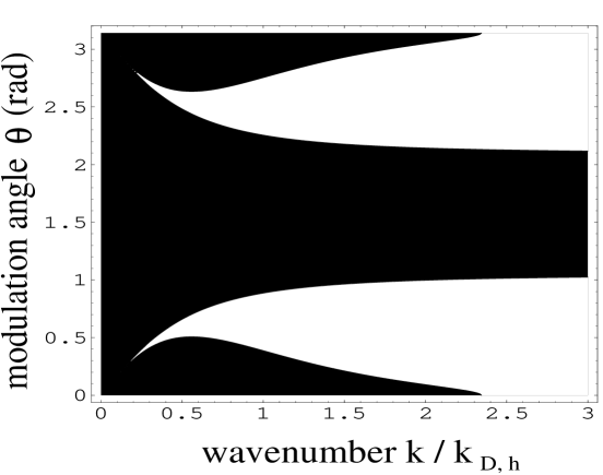
Figure 1:

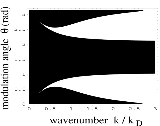
Figure 2:

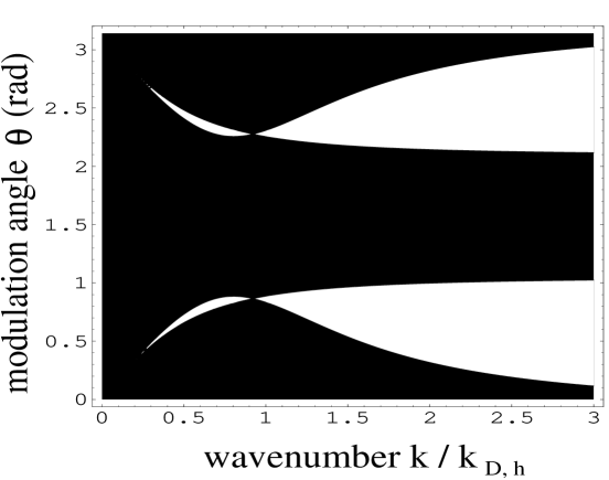
Figure 3:

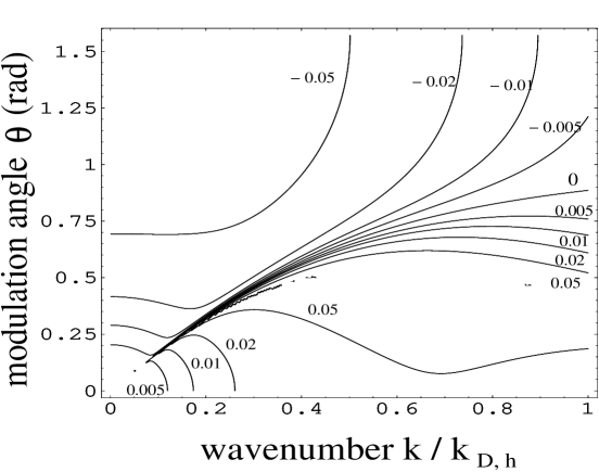
Figure 4:

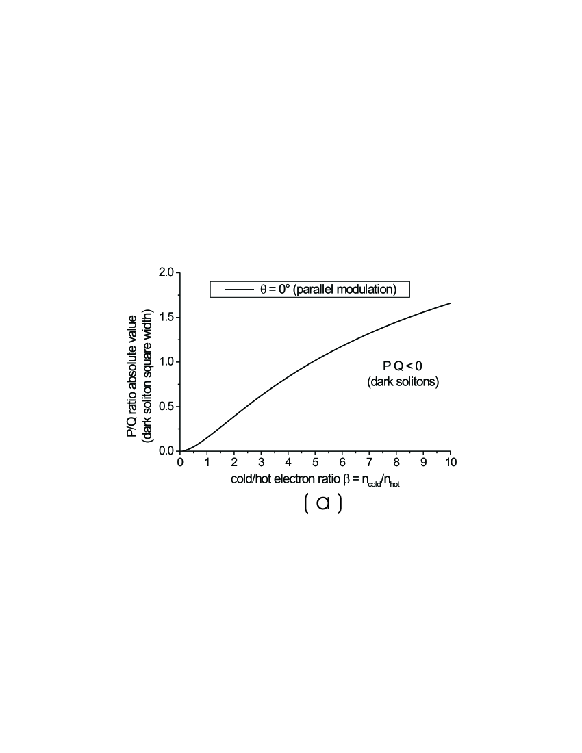
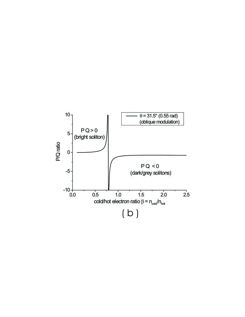
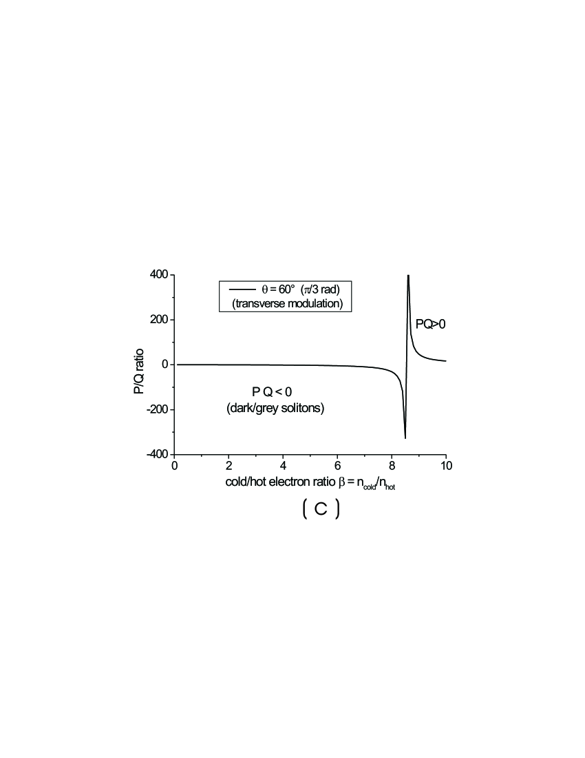
Figure 5: