Enhanced group velocity in metamaterials

Abstract. The Bruggeman formalism is implemented to estimate the refractive index of an isotropic, dielectric, homogenized composite medium (HCM). Invoking the well–known Hashin–Shtrikman bounds, we demonstrate that the group velocity in certain HCMs can exceed the group velocities in their component materials. Such HCMs should therefore be considered as metamaterials.

PACS numbers: 41.20.Jb, 42.25.Dd, 83.80.Ab

1 Introduction

By definition, metamaterials exhibit behavior which (i) either their component materials do not exhibit (ii) or is enhanced relative to exhibition in the component materials [1]. Many types of metamaterials may be conceptualized through the process of homogenization [2, 3, 4], paving the way for their realization. For example, a homogenized composite medium (HCM) may be envisaged which supports the propagation of a Voigt wave (which is a planar wave whose amplitude varies linearly with propagation distance), although such waves cannot propagate through its component materials [5, 6].

In this communication, we explore the enhancement of group velocity which may be achieved through homogenization. Sølna and Milton recently considered this issue, by estimating the relative permittivity of a HCM as the volume–weighted sum of the relative permittivities of the component materials [7]. But that estimation is applicable only for planar composite materials such as superlattices of thin films, and not to the more commonly encountered particulate composite materials [2, 3, 4]. In the following analysis, we implement the well–established Bruggeman formalism [4] to calculate the effective refractive index of an isotropic dielectric HCM. Thereby, we demonstrate that metamaterials which support group velocities exceeding those in their component materials may be realized as particulate composite materials.

2 Analysis

Consider a composite material containing materials labeled $a$ and $b$, with refractive indexes $n_{a}$ and $n_{b}$, respectively. The component materials are envisioned as random distributions of spherical particles. Provided that the diameters of these particles are small compared with electromagnetic wavelengths, homogenization techniques may be applied to estimate the effective refractive index of the HCM.

In particular, the well–established Bruggeman homogenization formalism [2, 4] — which may be rigorously derived from the strong–permittivity–fluctuation theory [8, 9] —  leads to the equation

$$f_{a}\frac{n^{2}_{a}-n^{2}_{Br}}{n^{2}_{a}+2n^{2}_{Br}}+f_{b}\frac{n^{2}_{b}-n^{2}_{Br}}{n^{2}_{b}+2n^{2}_{Br}}=0,$$ (1)

whose solution yields $n_{Br}$ as the estimated refractive index of the HCM. Here, $f_{a}$ and $f_{b}=1-f_{a}$ are the volume fractions of the component materials. In the following, both component materials are assumed to have negligible dissipation in the frequency range of interest.

The group velocity of a wavepacket propagating through the HCM is given as [10]

$$\left.v_{Br}=\frac{c}{n_{Br}(\omega)+\omega\frac{dn_{Br}}{d\omega}}\;\right|_{\omega(k_{avg})},\hskip 71.13188pt$$ (2)

where $v_{Br}$ is evaluated at the angular frequency $\omega=\omega(k_{avg})$, with $k_{avg}$ being the average wavenumber of the wavepacket, and $c$ is the speed of light in free space. Similarly, the respective group velocities in component materials $a$ and $b$ are given by

$$\left.v_{\ell}=\frac{c}{n_{\ell}(\omega)+\omega\frac{dn_{\ell}}{d\omega}}\;\right|_{\omega(k_{avg})},\hskip 71.13188pt\left(\ell=a,b\right).$$ (3)

We proceed to establish upper and lower bounds on $v_{Br}$, in terms of $n_{a}$ and $n_{b}$. In particular, we demonstrate that the inequalities

$$v_{Br}>v_{\ell}\,,\hskip 71.13188pt\left(\ell=a,b\right)$$ (4)

can be satisfied for certain values of $n_{a}\geq 1$, $n_{b}\geq 1$, $\frac{dn_{a}}{d\omega}>0$, and $\frac{dn_{b}}{d\omega}>0$.

Differentiation of both sides of Eq. (1) with respect to $\omega$ yields

$$\frac{dn_{Br}}{d\omega}=\delta_{a}\frac{dn_{a}}{d\omega}+\delta_{b}\frac{dn_{b}}{d\omega},$$ (5)

where

$$\left.\begin{array}[]{l}\delta_{a}=\displaystyle\frac{f_{a}n_{a}n_{Br}\left(n^{2}_{b}+2n^{2}_{Br}\right)^{2}}{f_{a}n^{2}_{a}\left(n^{2}_{b}+2n^{2}_{Br}\right)^{2}+f_{b}n^{2}_{b}\left(n^{2}_{a}+2n^{2}_{Br}\right)^{2}}\\ \vspace{-4mm}\\ \delta_{b}=\displaystyle\frac{f_{b}n_{b}n_{Br}\left(n^{2}_{a}+2n^{2}_{Br}\right)^{2}}{f_{a}n^{2}_{a}\left(n^{2}_{b}+2n^{2}_{Br}\right)^{2}+f_{b}n^{2}_{b}\left(n^{2}_{a}+2n^{2}_{Br}\right)^{2}}\end{array}\right\}.$$ (6)

Upper and lower bounds on $\delta_{a}$ and $\delta_{b}$ may be established by exploiting the Hashin–Shtrikman bounds $n_{L}$ and $n_{U}$ on $n_{Br}$ [11]; i.e.,

$$n_{L}<n_{Br}<n_{U},$$ (7)

where

$$\left.\begin{array}[]{l}n^{2}_{L}=n^{2}_{b}+\displaystyle\frac{3f_{a}n^{2}_{b}\left(n^{2}_{a}-n^{2}_{b}\right)}{n^{2}_{a}+2n^{2}_{b}-f_{a}\left(n^{2}_{a}-n^{2}_{b}\right)}\\ \vspace{-4mm}\\ n^{2}_{U}=n^{2}_{a}+\displaystyle\frac{3f_{b}n^{2}_{a}\left(n^{2}_{b}-n^{2}_{a}\right)}{n^{2}_{b}+2n^{2}_{a}-f_{b}\left(n^{2}_{b}-n^{2}_{a}\right)}\end{array}\right\}.$$ (8)

Combining Eqs. (6)–(8), we get

$$\rho_{\ell}<\delta_{\ell}<\kappa_{\ell}\,,\hskip 71.13188pt\left(\ell=a,b\right),$$ (9)

where

$$\left.\begin{array}[]{l}\kappa_{a}=\displaystyle\frac{f_{a}n_{a}n_{U}\left(n^{2}_{b}+2n^{2}_{U}\right)^{2}}{f_{a}n^{2}_{a}\left(n^{2}_{b}+2n^{2}_{L}\right)^{2}+f_{b}n^{2}_{b}\left(n^{2}_{a}+2n^{2}_{L}\right)^{2}}\\ \vspace{-4mm}\\ \kappa_{b}=\displaystyle\frac{f_{b}n_{b}n_{U}\left(n^{2}_{a}+2n^{2}_{U}\right)^{2}}{f_{a}n^{2}_{a}\left(n^{2}_{b}+2n^{2}_{L}\right)^{2}+f_{b}n^{2}_{b}\left(n^{2}_{a}+2n^{2}_{L}\right)^{2}}\end{array}\right\}$$ (10)

and

$$\left.\begin{array}[]{l}\rho_{a}=\displaystyle\frac{f_{a}n_{a}n_{L}\left(n^{2}_{b}+2n^{2}_{L}\right)^{2}}{f_{a}n^{2}_{a}\left(n^{2}_{b}+2n^{2}_{U}\right)^{2}+f_{b}n^{2}_{b}\left(n^{2}_{a}+2n^{2}_{U}\right)^{2}}\\ \vspace{-4mm}\\ \rho_{b}=\displaystyle\frac{f_{b}n_{b}n_{L}\left(n^{2}_{a}+2n^{2}_{L}\right)^{2}}{f_{a}n^{2}_{a}\left(n^{2}_{b}+2n^{2}_{U}\right)^{2}+f_{b}n^{2}_{b}\left(n^{2}_{a}+2n^{2}_{U}\right)^{2}}\end{array}\right\}.$$ (11)

Thus, we have

$$\rho_{a}\frac{dn_{a}}{d\omega}+\rho_{b}\frac{dn_{b}}{d\omega}<\frac{dn_{Br}}{d\omega}<\kappa_{a}\frac{dn_{a}}{d\omega}+\kappa_{b}\frac{dn_{b}}{d\omega},$$ (12)

and the group velocity in the HCM is accordingly bounded as

$$v_{L}<v_{Br}<v_{U}\,,$$ (13)

with

$$\left.\begin{array}[]{l}v_{L}=\displaystyle\frac{c}{n_{U}+\omega\left(\kappa_{a}\frac{dn_{a}}{d\omega}+\kappa_{b}\frac{dn_{b}}{d\omega}\right)}\\ \vspace{-4mm}\\ v_{U}=\displaystyle\frac{c}{n_{L}+\omega\left(\rho_{a}\frac{dn_{a}}{d\omega}+\rho_{b}\frac{dn_{b}}{d\omega}\right)}\end{array}\right\}.$$ (14)

If the inequalities

$$\left.\begin{array}[]{l}\displaystyle n_{U}+\omega\left(\kappa_{a}\frac{dn_{a}}{d\omega}+\kappa_{b}\frac{dn_{b}}{d\omega}\right)<n_{a}+\omega\frac{dn_{a}}{d\omega}\\ \vspace{-4mm}\\ \displaystyle n_{U}+\omega\left(\kappa_{a}\frac{dn_{a}}{d\omega}+\kappa_{b}\frac{dn_{b}}{d\omega}\right)<n_{b}+\omega\frac{dn_{b}}{d\omega}\end{array}\right\}$$ (15)

hold for certain component materials, then the inequalities (4) are automatically satisfied.

The inequalities (15) reduce to the particularly simple inequality

$$n_{U}+\omega\frac{dn_{a}}{d\omega}\left(\kappa_{a}+\kappa_{b}-1\right)+\kappa_{b}\left(n_{a}-n_{b}\right)<n_{a},$$ (16)

if $v_{a}=v_{b}$. The conditions

$$\left.\begin{array}[]{lcl}n_{U}+\kappa_{b}\left(n_{a}-n_{b}\right)&<&n_{a}\\ \vspace{-4mm}\\ \kappa_{a}+\kappa_{b}-1&>&0\end{array}\right\}$$ (17)

are satisfied, for example, by $n_{a}=3$, $n_{b}=1.2$ and $f_{a}=0.9$. Thus, the inequality (16) holds, provided that the dispersive term $\frac{dn_{a}}{d\omega}$ is sufficiently small.

3 Numerical results

Let us illustrate the phenomenon represented by the inequalities (4) by means of a specific numerical example. Consider a particulate composite material at a particular value $\omega_{\scriptscriptstyle 0}$ of $\omega$. At the chosen angular frequency, let $n_{a}=5$, $n_{b}=1.2$, $\frac{dn_{a}}{d\omega}\Big{|}_{\omega=\omega_{\scriptscriptstyle 0}}=0.5/\omega_{\scriptscriptstyle 0}$, and $\frac{dn_{b}}{d\omega}\Big{|}_{\omega=\omega_{\scriptscriptstyle 0}}=5.5/\omega_{\scriptscriptstyle 0}$. Significantly, material $a$ has a high refractive index but low dispersion in the neighbourhood of $\omega_{\scriptscriptstyle 0}$, whereas high dispersion in material $b$ is combined with a low refractive index.

The Bruggeman estimate of the refractive index of the HCM, namely $n_{Br}$, is plotted as a function of the volume fraction $f_{a}$ in figure 1. Also shown are the upper and lower Hashin–Shtrikman bounds, $n_{U}$ and $n_{L}$, on $n_{Br}$, as well as the parameters $\delta_{a}$ and $\delta_{b}$. The Bruggeman estimate adheres closely to the lower bound $n_{L}$ at low values of $f_{a}$, whereas at high values of $f_{a}$ the difference between $n_{Br}$ and its upper bound $n_{U}$ becomes marginal. The observed agreement between $n_{Br}$ and $n_{L}$ at low $f_{a}$ reflects the fact that the lower Hashin–Shtrikman bound is equivalent to the Maxwell Garnett estimate of the refractive index of the HCM arising from spherical particles of material $a$ embedded in the host material $b$ [4]. The Maxwell Garnett estimate is only valid then at low values of $f_{a}$. As the volume fraction becomes increasingly small, the Bruggeman estimate ($n_{Br}$) and the Maxwell Garnett estimate (low $f_{a}$ value of $n_{L}$) converge on $n_{b}$. In a similar manner, the agreement between $n_{Br}$ and $n_{U}$ at high values of $f_{a}$ is indicative of the fact that the upper Hashin–Shtrikman bound is equivalent to the Maxwell Garnett estimate of the refractive index of the HCM arising from spherical particles made of material $b$ embedded in host material $a$; the Maxwell Garnett estimate then holds only at high values of $f_{a}$. In the limit $f_{a}\rightarrow 0$, the coefficients $\delta_{a}\rightarrow 0$ and $\delta_{b}\rightarrow 1$; while $\delta_{a}\rightarrow 1$ and $\delta_{b}\rightarrow 0$ as $f_{a}\rightarrow 1$.

The corresponding group velocities $v_{a}$, $v_{b}$ and $v_{Br}$ are plotted as functions of $f_{a}$ in figure 2. The upper and lower bounds on $v_{Br}$ as given by $v_{U}$ and $v_{L}$, respectively, are also displayed. Clearly, we have $v_{Br}>v_{a}$ and $v_{Br}>v_{b}$ for $f_{a}>0.67$.

The inequalities (4) hold only over a relatively small range of parameter values. For example, the phase space in which the inequalities (4) are satisfied is illustrated in figure 3 for $n_{a}=5$, $\frac{dn_{a}}{d\omega}\Big{|}_{\omega=\omega_{\scriptscriptstyle 0}}=0.5/\omega_{\scriptscriptstyle 0}$ and $f_{a}=0.8$. With these relationships fixed for the component material $a$, we find that $v_{Br}>v_{a}$ and $v_{Br}>v_{b}$ for

• $1.17<n_{b}<1.23$ with $\frac{dn_{b}}{d\omega}\Big{|}_{\omega=\omega_{\scriptscriptstyle 0}}=5.51/\omega_{\scriptscriptstyle 0}$; and

• $5.45/\omega_{\scriptscriptstyle 0}<\frac{dn_{b}}{d\omega}\Big{|}_{\omega=\omega_{\scriptscriptstyle 0}}<5.57/\omega_{\scriptscriptstyle 0}$ with $n_{b}=1.2$.

4 Concluding remarks

We conclude that the group velocity in an isotropic, dielectric, particulate composite material — as estimated via the Bruggeman homogenization formalism — can exceed the group velocities in its component materials. This metamaterial characteristic may be achieved through homogenizing (i) a component material $a$ with high refractive index and low dispersion with (ii) a component material $b$ with low refractive index and high dispersion. Neither anomalous dispersion nor an explicit frequency–dependent model of the refractive index (unlike Ref. [7]) is required to demonstrate this characteristic.

Improved estimates of HCM group velocity may be achieved through the implementation of homogenization approaches which take into better account the distributional statististics of the component materials (e.g., the strong–permittivity–fluctuation theory approach [8, 9]). In particular, the effects of coherent scattering losses — which are neglected in the present study — may well result in a moderation of the group velocity. Such studies are currently being undertaken, especially in light of the recent emergence of metamaterials wherein the phase velocity and the time–averaged Poynting vector are oppositely directed [12].

Acknowledgements. TGM acknowledges the financial support of The Nuffield Foundation. AL thanks the Trustees of the Pennsylvania State University for a sabbatical leave of absence.

List of Figure Captions

Fig. 1. The estimated refractive index $n_{Br}$ (solid line), the upper and lower Hashin–Shtrikman bounds on $n_{Br}$ (broken dashed lines, labeled as $n_{U}$ and $n_{L}$), and the coefficients $\delta_{a}$ and $\delta_{b}$ (dashed lines), all plotted as functions of the volume fraction $f_{a}$, when $n_{a}=5$ and $n_{b}=1.2$.

Fig. 2. The estimated group velocity $v_{Br}$ (solid line) and its upper and lower bounds (broken dashed lines, labeled as $v_{U}$ and $v_{L}$), along with the group velocities $v_{a}$ and $v_{b}$ (broken dashed lines) in the component materials, plotted as functions of the volume fraction $f_{a}$, when $n_{a}=5$, $n_{b}=1.2$, $\frac{dn_{a}}{d\omega}\Big{|}_{\omega=\omega_{\scriptscriptstyle 0}}=0.5/\omega_{\scriptscriptstyle 0}$ and $\frac{dn_{b}}{d\omega}\Big{|}_{\omega=\omega_{\scriptscriptstyle 0}}=5.5/\omega_{\scriptscriptstyle 0}$. All group velocities are normalized with respect to $c$.

Fig. 3. The shaded region indicates the portion of the $\alpha$–$\beta$ phase space wherein $v_{Br}>v_{a}$ and $v_{Br}>v_{b}$; here, $\alpha=\frac{n_{a}}{n_{b}}$ and $\beta=\Big{(}\frac{dn_{a}}{d\omega}/\frac{dn_{b}}{d\omega}\Big{)}\Big{|}_{\omega=\omega_{\scriptscriptstyle 0}}$. This region was demarcated for $n_{a}=5$, $\frac{dn_{a}}{d\omega}\Big{|}_{\omega=\omega_{\scriptscriptstyle 0}}=0.5/\omega_{\scriptscriptstyle 0}$ and $f_{a}=0.8$.

Figure 1: The estimated refractive index $n_{Br}$ (solid line), the upper and lower Hashin–Shtrikman bounds on $n_{Br}$ (broken dashed lines, labeled as $n_{U}$ and $n_{L}$), and the coefficients $\delta_{a}$ and $\delta_{b}$ (dashed lines), all plotted as functions of the volume fraction $f_{a}$ when $n_{a}=5$ and $n_{b}=1.2$.

Figure 2: The estimated group velocity $v_{Br}$ (solid line) and its upper and lower bounds (broken dashed lines, labeled as $v_{U}$ and $v_{L}$), along with the group velocities $v_{a}$ and $v_{b}$ (broken dashed lines) in the component materials, plotted as functions of the volume fraction $f_{a}$, when $n_{a}=5$, $n_{b}=1.2$, $\frac{dn_{a}}{d\omega}\Big{|}_{\omega=\omega_{\scriptscriptstyle 0}}=0.5/\omega_{\scriptscriptstyle 0}$ and $\frac{dn_{b}}{d\omega}\Big{|}_{\omega=\omega_{\scriptscriptstyle 0}}=5.5/\omega_{\scriptscriptstyle 0}$. All group velocities are normalized with respect to $c$.

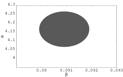
Figure 3: The shaded region indicates the portion of the $\alpha$–$\beta$ phase space wherein $v_{Br}>v_{a}$ and $v_{Br}>v_{b}$; here, $\alpha=\frac{n_{a}}{n_{b}}$ and $\beta=\Big{(}\frac{dn_{a}}{d\omega}/\frac{dn_{b}}{d\omega}\Big{)}\Big{|}_{\omega=\omega_{\scriptscriptstyle 0}}$. This region was demarcated for $n_{a}=5$, $\frac{dn_{a}}{d\omega}\Big{|}_{\omega=\omega_{\scriptscriptstyle 0}}=0.5/\omega_{\scriptscriptstyle 0}$ and $f_{a}=0.8$.

References

• [1] Walser RM 2003 Metamaterials Introduction to Complex Mediums for Optics and Electromagnetics Weiglhofer WS and Lakhtakia A (eds) ( Bellingham, WA, USA: SPIE Optical Engineering Press)
• [2] Ward L 1988 The Optical Constants of Bulk Materials and Films (Bristol, UK: Adam Hilger)
• [3] Neelakanta PS 1995 Handbook of Electromagnetic Materials ( Boca Raton, FL, USA: CRC Press)
• [4] Lakhtakia A (ed) 1996 Selected Papers on Linear Optical Composite Materials ( Bellingham, WA, USA: SPIE Optical Engineering Press)
• [5] Mackay TG and Lakhtakia A 2003 Voigt wave propagation in biaxial composite materials J. Opt. A: Pure Appl. Opt. 5 91
• [6] Mackay TG and Lakhtakia A 2004 Correlation length facilitates Voigt wave propagation Waves Random Media 14 L1
• [7] Sølna K and Milton GW 2002 Can mixing materials make electromagnetic signals travel faster? SIAM J. Appl. Math. 62 2064
• [8] Kong JA and Tsang L 1981 Scattering of electromagnetic waves from random media with strong permittivity fluctuations Radio Sci. 16 303
• [9] Mackay TG 2003 Homogenization of linear and nonlinear complex composite materials Introduction to Complex Mediums for Optics and Electromagnetics Weiglhofer WS and Lakhtakia A (eds) (Bellingham, WA, USA: SPIE Optical Engineering Press)
• [10] Jackson JD 1999 Classical Electrodynamics (3rd edn) (New York, NY, USA: John Wiley & Sons)
• [11] Hashin Z and Shtrikman S 1962 A variational approach to the theory of the effective magnetic permeability of multiphase materials J. Appl. Phys. 33 3125
• [12] Lakhtakia A, McCall MW, and Weiglhofer WS 2003 Negative phase–velocity mediums Introduction to Complex Mediums for Optics and Electromagnetics ed WS Weiglhofer and A Lakhtakia (Bellingham, WA, USA: SPIE Optical Engineering Press)