Permanent address: ]Rutherford Appleton Laboratory, Chilton, Didcot, Oxfordshire, OX11 0QX, UK

Nonlinear model for magnetosonic shocklets in plasmas

Abstract

Exact nonlinear equations for magnetosonic shocklets in a uniform hot magnetoplasma are derived by using the nonlinear magnetohydrodynamic equations. Analytic as well as numerical solutions of the nonlinear equations are presented. Shock-like structures of the ion fluid velocity and magnetic field (or the plasma density) perturbations are obtained. The results may have relevance to the understanding of fast magnetosonic shocklets that have been recently observed by onboard instruments of the Cluster spacecraft at the Earth’s bow shock.

In the past, there has been a great deal of theoretical interest (e.g. Refs. r0 ; r1 ; r2 ) in studying the properties of nonlinear magnetohydrodynamic waves in plasmas. It has been found that both slow and fast magnetosonic (FMS) waves can propagate in the form of either solitary or shock waves in plasmas. Very recently Stasiewicz et al. a0 ; a1 reported detailed properties of slow magnetosonic (SM) solitons a0 and FMS shocklets a1 , which have been observed by a fleet of four Cluster spacecraft at the quasi-parallel bow shock. Observations reveal that SM solitons jm are associated with large amplitude compressional (rarefactional) magnetic field (plasma density) variations. On the other hand, FMS shocklets are accompanied with compression of the plasma density and magnetic field perturbations.

In this Brief Communication, we present a nonlinear model for FMS shocklets, which may account for the observed FMS shocklets at the Earth’s bow shock. Specifically, we show that FMS shocklets are associated with the nonlinear steepening r3 of arbitrary large amplitude FMS waves in a high-beta magnetoplasma.

The dynamics of the nonlinear FMS waves in a magnetized plasma is governed by the inertialess electron momentum equation

$$0=-n_{e}e{\bf E}-\nabla p_{e}-n_{e}e\frac{{\bf v}_{e}}{c}\times{\bf B},$$ (1)

where $n_{e}$ is the electron density, $e$ is the magnitude of the electron charge, ${\bf E}$ is the wave electric field, ${\bf B}$ is the sum of the ambient and wave magnetic fields, $p_{e}=n_{e}T_{e}$ is the electron pressure, $T_{e}$ is the electron temperature, ${\bf v}_{e}$ is the electron fluid velocity, and $c$ is the speed of light in vacuum. The ion dynamics is governed by the ion continuity equation

$$\frac{\partial n_{i}}{\partial t}+\nabla\cdot(n_{i}{\bf v}_{i})=0,$$ (2)

and the ion momentum equation

$$\rho\left(\frac{\partial}{\partial t}+{\bf v}_{i}\cdot\nabla\right){\bf v}_{i}=n_{i}e{\bf E}-\nabla p_{i}+n_{i}e\frac{{\bf v}_{i}}{c}\times{\bf B},$$ (3)

where $n_{i}$ is the ion number density, ${\bf v}_{i}$ is the ion fluid velocity, $\rho=n_{i}m_{i}$ is the ion mass density, $m_{i}$ is the ion mass, $p_{i}=n_{i}T_{i}$ is the ion pressure, and $T_{i}$ is the ion temperature. Equations (1)-(3) are closed by means of Ampère’s and Faraday’s laws

$$\nabla\times{\bf B}=\frac{4\pi e}{c}(n_{i}{\bf v}_{i}-n_{e}{\bf v}_{e}),$$ (4)

$$\frac{\partial{\bf B}}{\partial t}=-c\nabla\times{\bf E},$$ (5)

together with the quasi-neutrality condition $n_{e}=n_{i}=n$. The latter is valid for a dense plasma in which the ion plasma frequency is much larger than the ion gyrofrequency. Equation (4) holds for the FMS waves whose phase speed is much smaller than the speed of light.

Eliminating ${\bf E}$ from (1) and (3) we obtain

$$\frac{\partial{\bf v}_{i}}{\partial t}+{\bf v}_{i}\cdot\nabla{\bf v}_{i}=\frac{(\nabla\times{\bf B})\times{\bf B}}{4\pi\rho}-C_{s}^{2}\nabla{\rm ln}\,\rho,$$ (6)

where the ion sound speed is denoted by $C_{s}=[(T_{e}+T_{i})/m_{i}]^{1/2}$. On the other hand, from (1), (4) and (5) we have

$$\frac{\partial{\bf B}}{\partial t}=\nabla\times\left[{\bf v}_{i}\times{\bf B}-\frac{c}{4\pi en}(\nabla\times{\bf B})\times{\bf B}\right].$$ (7)

We are interested in studying the nonlinear properties of one-dimensional FMS waves across the external magnetic field direction $\hat{\bf z}B_{0}$, where $\hat{\bf z}$ is the unit vector along the $z$ axis and $B_{0}$ is the strength of the ambient magnetic field. Thus, we have $\nabla=\hat{\bf x}\partial/\partial x$, ${\bf v}_{i}=u\hat{\bf x}$ and ${\bf B}=B(x)\hat{\bf z}$, where $\hat{\bf x}$ is the unit vector along the $x$ axis in the Cartesian coordinate. Normalizing $\rho$ by the equilibrium mass density $\rho_{0}=n_{0}m_{i}$, $u$ by the Alfvén speed $V_{A}=B_{0}/\sqrt{4\pi\rho_{0}}$, $B$ by $B_{0}$, time by the ion gyroperiod $\omega_{ci}^{-1}$, $x$ by $V_{A}/\omega_{ci}=c/\omega_{pi}$, where $\omega_{pi}$ is the ion plasma frequency, we have our nonlinear MHD equations in dimensionless form as

$$\frac{\partial\rho}{\partial t}+\frac{\partial}{\partial x}(\rho u)=0,$$ (8)

$$\frac{\partial u}{\partial t}+u\frac{\partial u}{\partial x}+\frac{1}{\rho}\frac{\partial}{\partial x}\left(\frac{h^{2}}{2}+\beta\,\rho\right)=0,$$ (9)

and

$$\frac{\partial h}{\partial t}+h\frac{\partial u}{\partial x}+u\frac{\partial h}{\partial x}=0,$$ (10)

where $h=B(x,t)/B_{0}$ and $\beta=C_{s}^{2}/V_{A}^{2}\equiv 4\pi n_{0}(T_{e}+T_{i})/B_{0}^{2}$ represents the plasma beta.

Equations (8) and (10) yield $\rho=h$, a concept of frozen-in-field lines in a magnetized plasma. Hence, we have from (9) and (10)

$$\frac{\partial u}{\partial t}+u\frac{\partial u}{\partial x}+\frac{\partial}{\partial x}\left(h+\beta\,{\rm ln}\,h\right)=0,$$ (11)

and

$$\frac{\partial h}{\partial t}+u\frac{\partial h}{\partial x}+h\frac{\partial u}{\partial x}=0.$$ (12)

In the zero-$\beta$ limit, Eqs. (11) and (12) agree completely with Eqs. (2a) and (2b) of Stenflo et al. a2 who demonstrated rapid steepening of the velocity and magnetic field perturbations leading to the formation of FMS shocklets in a cold magnetoplasma.

In the following, we study the properties of FMS shocklets in a warm magnetoplasma. We introduce the change of variables

$$\psi_{1} = u+2\sqrt{h+\beta}+\sqrt{\beta}\mathrm{ln}\left(\frac{\sqrt{h+\beta}-\sqrt{\beta}}{\sqrt{h+\beta}+\sqrt{\beta}}\right)+c_{1},$$ (13)

$$\psi_{2} = -u+2\sqrt{h+\beta}+\sqrt{\beta}\mathrm{ln}\left(\frac{\sqrt{h+\beta}-\sqrt{\beta}}{\sqrt{h+\beta}+\sqrt{\beta}}\right)+c_{2},$$ (14)

where $c_{1}$ and $c_{2}$ are constants. This diagonalizes the system of equations (11)–(12) to the form

$$\frac{\partial\psi_{1}}{\partial t}+(u+\sqrt{h+\beta})\frac{\partial\psi_{1}}{\partial x}=0,$$ (15)

$$\frac{\partial\psi_{2}}{\partial t}+(u-\sqrt{h+\beta})\frac{\partial\psi_{2}}{\partial x}=0,$$ (16)

where $u$ and $h$ are given in terms of $\psi_{1}$ and $\psi_{2}$ by Eqs. (13)–(14). This system admits “simple wave” solutions a6 , which can be found by either setting $\psi_{1}$ or $\psi_{2}$ to zero. Setting $\psi_{2}$ to zero in Eqs. (15)–(16), we obtain

$$\frac{\partial\psi_{1}}{\partial t}+(u+\sqrt{h+\beta})\frac{\partial\psi_{1}}{\partial x}=0,$$ (17)

where from Eqs. (13)–(14)

$$u=2\sqrt{h+\beta}+\sqrt{\beta}\mathrm{ln}\left(\frac{\sqrt{h+\beta}-\sqrt{\beta}}{\sqrt{h+\beta}+\sqrt{\beta}}\right)+c=\frac{\psi_{1}}{2}.$$ (18)

The constant

$$c=-2\sqrt{1+\beta}-\sqrt{\beta}\ln\left(\frac{\sqrt{1+\beta}-\sqrt{\beta}}{\sqrt{1+\beta}+\sqrt{\beta}}\right)$$

is determined by the boundary conditions $u=0$ and $h=1$ at $|x|=\infty$. Using $\psi_{1}=2u$ in Eq. (17), we have

$$\frac{\partial u}{\partial t}+(u+\sqrt{h+\beta})\frac{\partial u}{\partial x}=0,$$ (19)

where $h(u)$ is implicitly given by Eq. (18). We note that the results given by Eqs. (18) and (19) generalize the results presented in Ref. a2 for the case of arbitrary $\beta$ values. The paths in the ($x,t$) space where $u$ is constant, can be described by the ordinary differential equation

$$\frac{dx}{dt}=u+\sqrt{h+\beta},$$ (20)

where the right-hand side is constant (since $u$ is constant along the path), which after integration gives

$$x(t)=(u+\sqrt{h+\beta})t+x_{0}.$$ (21)

Here $x_{0}$ is a constant of integration. The general solution of Eq. (19) is a function of the integration constant $x_{0}$, viz.

$$u=f(x_{0})=f[x-(u+\sqrt{h+\beta})t],$$ (22)

where $h(u)$ is given by Eq. (18) and $f$ is a function of one variable, determined from the initial condition at $t=0$; the velocity $u$ can be evaluated for different $x$ and $t$ by solving Eq. (22) for $u$. Equation (22) describes a nonlinear FMS wave propagating in the positive $x$ direction, where the time-dependent solution has a typical structure of the wave-steepening, similarly to the solution of the inviscid Burgers equation r1 . This solution may also be obtained by directly assuming that $h$ can be written as a function of $u$. Note that there are no steady state solutions within this system, since the dispersion is absent; but by including the electron inertial effect in Eq. (10) this could be achieved on length scales $\lesssim\lambda_{e}=c/\omega_{pe}$, where $\omega_{pe}$ is the electron plasma frequency. The dispersive effects break the $\rho=h$ relation, and produce an asymmetry between the density and magnetic field perturbations.

We have analyzed the system (11)–(12) numerically. As an initial condition, we took the magnetic field $h=1+0.5\,\mathrm{sech}(x/20)$, describing a localized magnetic field (and density) compression of the plasma. As we are interested in the evolution and creation of a “shocklet” moving in one direction, we choose the initial condition for the velocity $u$ from Eq. (18), describing a wave moving in the positive $x$–direction only. The evolution of the system for a low-beta ($\beta=0$) and for a high-beta ($\beta=10$) plasma is displayed in Figs. 1 and 2, respectively. In agreement with the analytical prediction, the initial wave is propagating in the positive $x$–direction only. Figure 1 shows that both the magnetic and velocity perturbations steepen and a shock front starts to develop. For the high-beta plasma case, as displayed in Fig. 2, the velocity associated with the shocklet is larger, and the self-steepening develops faster than for the low-beta plasma case. When the shock fronts become steep enough, effects such as the electron inertia and electron Landau damping (which heats the plasma) will become important. Dispersive effects also occur if the waves propagate with some angle to the magnetic field direction. The combined effects of dispersion and wave-particle induced dissipation could explain the apparent phase asymmetry between the magnetic field and density perturbations, as observed in large-amplitude FMS shocklets a1 . This asymmetry is likely to appear after the shocklets have developed due to the self-steepening of the FMS waves, as investigated here.

To summarize, we have considered the nonlinear propagation of FMS waves in a hot magnetoplasma. It has been shown that the nonlinear MHD equations in a finite-$\beta$ plasma can be reduced to a pair of equations in which the ion fluid velocity and the compressional magnetic field are nonlinearly coupled. The system has been diagonalized and special, single wave solutions have been obtained. The solutions represent the spatio-temporal evolution of an arbitrary amplitude FMS waves. The equations for the full system are solved numerically to show the formation of FMS shocklets, in full agreement with the analytic results. The finite plasma beta has significant influence on the shocklet profile in that the shocks develop on a much shorter timescale than for the the plasma with a low beta. In conclusion, the present results qualitatively account for the salient features of the observed FMS shocklets at the Earth’s bow shock a1 .

FIGURE CAPTIONS

FIG. 1. The evolution of the normalized ion fluid velocity (upper panel) and compressional magnetic field (lower panel) for $\beta=0$, for the times 1) $t=0$, 2) $t=12.25$ 3) $t=24.75$ and 4) $t=37.25$.

FIG. 2. The evolution of the normalized ion fluid velocity (upper panel) and compressional magnetic field (lower panel) for $\beta=10$, for the times 1) $t=0$, 2) $t=12.25$ and 3) $t=24.75$.

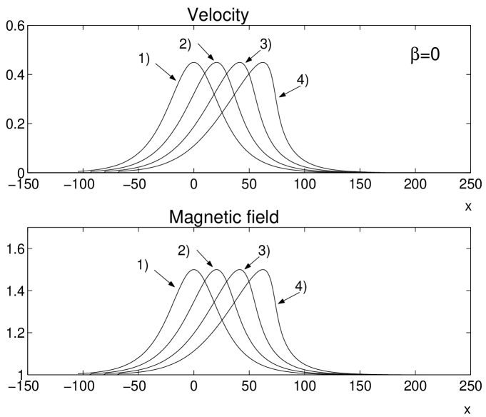
Figure 1:

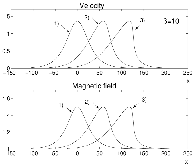
Figure 2: