On the intermittency exponent of the turbulent energy cascade

Abstract

We consider the turbulent energy dissipation from one-dimensional records in experiments using air and gaseous helium at cryogenic temperatures, and obtain the intermittency exponent via the two-point correlation function of the energy dissipation. The air data are obtained in a number of flows in a wind tunnel and the atmospheric boundary layer at a height of about 35 m above the ground. The helium data correspond to the centerline of a jet exhausting into a container. The air data on the intermittency exponent are consistent with each other and with a trend that increases with the Taylor microscale Reynolds number, $R_{\lambda}$, of up to about 1000 and saturates thereafter. On the other hand, the helium data cluster around a constant value at nearly all $R_{\lambda}$, this being about half of the asymptotic value for the air data. Some possible explanation is offered for this anomaly.

I Introduction

That turbulent energy dissipation is intermittent in space has been known since the seminal work of Batchelor & Townsend BT . The characteristics of intermittency are best expressed, at present, in terms of multifractals and the multiplicity of scaling exponents; see e.g. Ref. MEN91 . In the hierarchy of the scaling exponents, the so-called intermittency exponent characterizing the second-order behavior of the energy dissipation, is the most basic. In this paper, we address the Reynolds number variation of the intermittency exponent and its asymptotic value (if one exists).

The intermittency exponent has been determined by a number of authors in the past using several different methods; for a summary as of some years ago, see Refs. SRE93 ; PRA97 . Recently, Cleve, Greiner & Sreenivasan CLE03a evaluated these methods and showed that the best procedure is to examine the scaling of the two-point correlation function $\langle\varepsilon(x+d)\varepsilon(x)\rangle$ of the energy dissipation $\varepsilon$. Other procedures based on moments $\langle\varepsilon_{l}^{2}\rangle$ and $\langle\ln^{2}\varepsilon_{l}\rangle-\langle\ln\varepsilon_{l}\rangle^{2}$ of the coarse-grained dissipation $\varepsilon_{l}=(1/l)\int_{l}\varepsilon(x)\mathrm{d}x$, or the power-spectrum $P(k)=|\varepsilon(k)|^{2}$, are corrupted by the unavoidable surrogacy of the observed energy dissipation.

The follow-up effort CLE03b was able to characterize and understand the functional form of the two-point correlation function beyond the power-law scaling range. Within the theory of (binary) random multiplicative cascade processes, the finite-size parametrization

$$\frac{\left\langle\varepsilon(x+d)\varepsilon(x)\right\rangle}{\left\langle\varepsilon(x)\right\rangle^{2}}=c\left(\frac{L_{\mathrm{casc}}}{d}\right)^{\mu}+(1-c)\frac{d}{L_{\mathrm{casc}}}$$ (1)

was derived, introducing the cascade length $L_{\mathrm{casc}}$ as a meaningful physical upper length scale, this being similar to the integral scale (as discussed later) but typically larger. Here, $\mu$ is the intermittency exponent, and the first term is the pure power-law part and the second term is the finite-size correction. Comments on the constant $c$ will be given further below. The one atmospheric and the three wind tunnel records employed in Ref. CLE03b were found to be in accordance with this close-to-universal finite-size parametrization. Even for flows at moderate Taylor-microscale Reynolds numbers $R_{\lambda}$, Eq. (1) allowed an unambiguous extraction of $\mu$. For the four data records, a weak dependence of $\mu$ on $R_{\lambda}$ was observed in CLE03b but was not commented upon in any detail. The present analysis examines many more records and attempts to put that Reynolds number dependence on firmer footing.

II The data

Two of the data records examined here come from the atmospheric boundary layer (records a1 and a2) DHR00 , eight records from a wind tunnel shear flow (records w1 to w8) PEA02 and eleven records from a gaseous helium jet flow (records h1 to h11) CHA00 . We find that all air experiments show an increasing trend of the exponent towards 0.2 as the Reynolds number increases. The helium data, on the other hand, show the exceptional behavior of a Reynolds-number-independent “constant” of around 0.1. Some comments on this behavior are made.

It is useful to summarize the standard analysis in order to emphasize the quality of the data. As is the standard practice, energy dissipation is constructed via its one-dimensional surrogate

$$\varepsilon(x)=15\nu\left(\frac{du}{dx}\right)^{2}\;,$$ (2)

where the coordinate system is defined such that $u$ is the component of the turbulent velocity pointing in the longitudinal $x$ direction (the direction of mean motion). The coefficient $\nu$ is the kinematic viscosity. Characteristic quantities such as the Reynolds number $R_{\lambda}\equiv\sqrt{\langle u^{2}\rangle}\lambda/\nu$, based on the Taylor microscale $\lambda=\sqrt{\langle u^{2}\rangle/\langle(\partial u/\partial x)^{2}\rangle}$, the integral length $L$, the record length $L_{\mathrm{record}}$, the resolution length $\Delta{x}$ and the hot-wire length $l_{w}$ in units of the Kolmogorov dissipation scale $\eta=(\nu^{3}/\langle\varepsilon\rangle)^{1/4}$ are listed in Table 1.

Table 1: Taylor-microscale based Reynolds number $R_{\lambda}$, the integral length scale $L$ in units of the Kolmogorov scale $\eta$, the record length $L_{\mathrm{record}}$, the Taylor microscale $\lambda$, the resolution scale $\Delta x$ ($=$ sampling time interval $\times$ mean velocity), the length of the hot wire $l_{w}$, the intermittency exponent $\mu$, the cascade length $L_{\mathrm{casc}}$ and the surrogacy cutoff length $\Lambda^{*}$ for the two atmospheric boundary layer data (a1,a2) DHR00 , the eight wind tunnel data (w1–w8) PEA02 and the eleven sets from gaseous helium jet (h1–h11) CHA00 measurements.

data set	$R_{\lambda}$	$L/\eta$	$L_{\mathrm{record}}/L$	$\lambda/\eta$	$\Delta x/\eta$	$l_{w}/\eta$	$\mu$	$L_{\mathrm{casc}}/\eta$	$\Lambda^{*}/\eta$
a1	$9000$	$5{\times}10^{4}$	$1000$	$187$	$1.29$	$1.755$	$0.216$	$322743$	$3.9$
a2	$17000$	$7.5{\times}10^{4}$	$970$	$246$	$3.64$	$1.534$	$0.202$	$509354$	$9.1$
w1	$208$	$539$	$28000$	$27$	$2.42$	$1.052$	$0.143$	$1164$	$24$
w2	$306$	$484$	$102500$	$35$	$1.98$	$1.780$	$0.155$	$1939$	$26$
w3	$410$	$697$	$127700$	$38$	$2.67$	$2.533$	$0.151$	$2707$	$27$
w4	$493$	$968$	$193500$	$44$	$2.79$	$3.382$	$0.145$	$3228$	$31$
w5	$584$	$1095$	$88600$	$44$	$2.71$	$0.890$	$0.172$	$4062$	$27$
w6	$704$	$1365$	$117700$	$48$	$2.90$	$1.079$	$0.173$	$4343$	$29$
w7	$860$	$1959$	$89500$	$53$	$2.63$	$1.580$	$0.176$	$5513$	$26$
w8	$1045$	$2564$	$77500$	$64$	$2.97$	$1.927$	$0.171$	$7469$	$27$
h1	$85$	$102$	$197000$	$22$	$1.20$	$0.040$	$0.12$	$934$	$10.8$
h2	$89$	$101$	$175000$	$22$	$1.05$	$0.025$	$0.128$	$472$	$10.5$
h3	$124$	$165$	$100000$	$26$	$0.98$	$0.068$	$0.102$	$738$	$17.7$
h4	$208$	$344$	$85200$	$33$	$1.75$	$0.088$	$0.154$	$1258$	$14.0$
h5	$209$	$277$	$59000$	$23$	$0.97$	$0.072$	$0.083$	$1559$	$10.7$
h6	$352$	$606$	$62400$	$47$	$2.25$	$0.165$	$0.13$	$2254$	$22.5$
h7	$463$	$1011$	$32100$	$50$	$1.93$	$0.310$	$0.092$	$10438$	$25.1$
h8	$885$	$1442$	$40100$	$47$	$3.45$	$0.763$	$0.089$	$18954$	$10.3$
h9	$929$	$2064$	$29800$	$48$	$3.67$	$0.762$	$0.079$	$8434$	$18.3$
h10	$985$	$2144$	$37800$	$48$	$4.83$	$0.837$	$0.105$	$23659$	$14.5$
h11	$1181$	$3106$	$26900$	$57$	$4.97$	$1.097$	$0.061$	$14921$	$19.9$

To calculate the numerical value of $\lambda$ the method described in ARO93 has been used. The integral length is defined as the integral over the velocity autocorrelation function (using Taylor’s hypothesis). In the atmosphere, where the data do not converge for very large values of the time lag, the autocorrelation function is smoothly extrapolated to zero and the integral is evaluated. This smoothing operation towards the tail does not introduce measurable uncertainty in $L$. The energy spectrum, which is illustrated in Fig. 1 for the records a2, w1 and h7 as representatives of the three different flow geometries with Reynolds numbers ranging from the small to the very large side, follows an approximate $-5/3$-rds power over the inertial range.

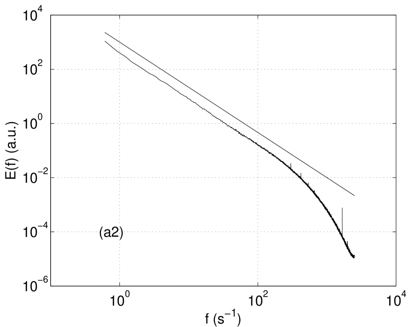
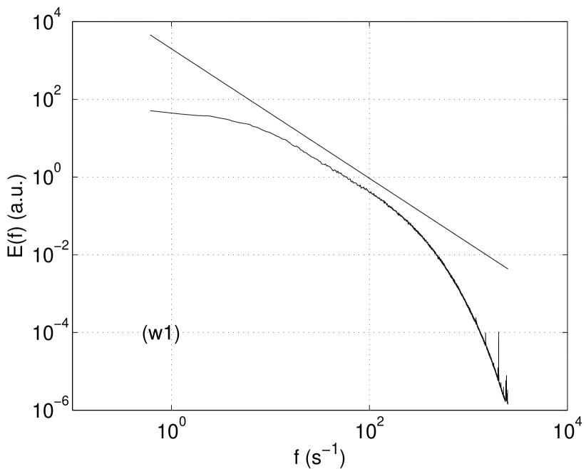
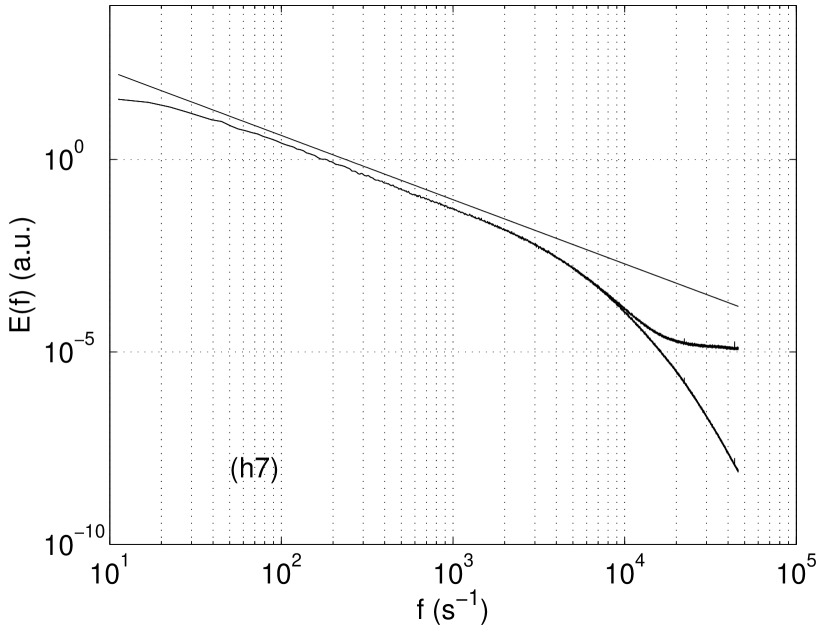
Figure 1: Power spectral densities of the velocity fluctuations for the records a2, w1 and h7. The sharp peaks are artifacts. For the record h7, the filtered power spectral density is also shown.

The wind tunnel records are relatively noise-free, while the helium data are affected by instrumental noise significantly, as evidenced by the flattening of the energy spectrum for high wave numbers. The atmospheric data fall somewhere in-between. The effect of this high-frequency noise, and of removing it by a suitable filtering scheme, will be discussed later.

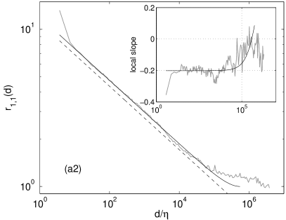
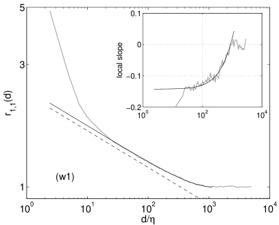
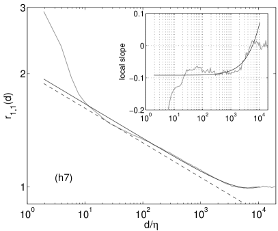
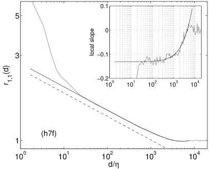
Figure 2: Best fits of expression (1) to two-point correlators extracted from data sets a2, w1, unfiltered h7 and filtered h7 (h7f). The inset figures show the local slopes, compared with the fits given by (1). For comparison, power-law fits with the extracted intermittency exponent listed in Table I (and $\mu=0.13$ for h7f) are shown as dashed straight lines drawn with arbitrary shifts.

Again for the three representative cases a2, w1 and h7, Fig. 2 shows the two-point correlation defined in (1) for the surrogate quantity (2) and compares it to the best-fits for the proposed form of finite-size parametrization given by Eq. (1). As is also the case for all the other records, the agreement is quite substantial and unambiguous. The upturn at small separation distances $d<\Lambda^{*}$ has been explained in CLE03a as the effect of the surrogacy of the energy dissipation. Hence, we call $\Lambda^{*}$ the surrogacy cutoff length. The two-point function decorrelates at a length scale $L_{\mathrm{casc}}$ that is substantially larger than the integral length scale. The cascade length $L_{\mathrm{casc}}$ and the surrogacy cutoff length $\Lambda^{*}$ are also listed in Table 1 for all the records inspected.

III Intermittency exponent

To determine the intermittency exponent $\mu$, the data are fitted to Eq. (1) using a best-fit algorithm (see Fig. 2). These values are also listed in Table 1. The local slopes from the best fits, plotted as insets in the figure, show that deviations from the pure power-law become evident only towards large values of the separation distance $d$. The dashed lines in each figure are pure power-laws (with arbitrary shift) for the values of $\mu$ listed in the Table.

For the atmospheric boundary layer, the analysis of two data sets yields a value of about $0.2$ for the intermittency exponent $\mu$; see Fig. 3.

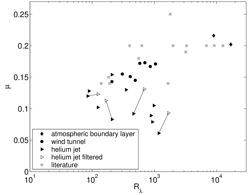
Figure 3: The intermittency exponent, $\mu$, extracted from a best fit of expression (1) to the two-point correlator of the various data records, as a function of the Taylor-microscale based Reynolds number. Also shown are some values quoted in the literature. For some of the helium data, the lines show the shift resulting from the application of the Wiener filter to remove high-frequency noise.

Note that, since the data set a1 contains both the longitudinal and transverse velocity components, one can form different forms of the surrogate energy dissipation. It was found in Ref. CLE03a that all of them lead to the same value of the intermittency exponent. The filtering of the data has no measurable effect on the numerical value of $\mu$.

The wind-tunnel data w1-w8 seem to suggest a Reynolds number dependence of the intermittency exponent for $R_{\lambda}$ of up to about 1000. The value $\mu=0.2$ of the atmospheric boundary layer is reached only for higher $R_{\lambda}$. Unfortunately there is no laboratory data for $R_{\lambda}>1000$ so that there is a gap between the wind tunnel data and the atmospheric boundary layer data. Nevertheless, all the air data taken together appear to be consistent with a trend that increases with the Taylor microscale Reynolds number up to an $R_{\lambda}$ of about 1000, and saturates thereafter. This trend is also supported by results quoted in the literature ANT81 ; ANT82 ; ANS84 ; KUZ92 ; SRE93 ; PRA97 ; MIJ01 , although the finite-size form (1) has not been employed for the extraction of the intermittency exponent. The literature values, shown in Fig. 3, fill the gap between the present wind tunnel and atmospheric data.

In contrast to the air data, the gaseous helium records h1-h11 show a different behavior (Fig. 3). It appears that, unlike the air data which show a gradual trend with $R_{\lambda}$, leading to a saturation for $R_{\lambda}>1000$, the helium data yield an intermittency exponent that is flat with $R_{\lambda}$ at a lower value of $0.1$. It remains an open question as to why this is so. It would be important to settle this puzzle and clarify if this special behavior has other consequences for the helium jet data.

To make some progress, we examined the helium data more closely. Perhaps the instrumental noise, which is seen in Fig. 1c by the flattening of the energy spectrum for high frequencies, affects the accuracy of the calculation of the energy dissipation. To account for such effects, we applied a Wiener filter to the data, see again Fig. 1c, and recomputed the two-point correlation; the result is shown in Fig. 2d. The quality of the agreement with the finite-size parametrization remained the same but the numerical value for the intermittency exponent altered. Filtering produces different amounts of shift for different sets of data; see again Fig. 3. The most extreme change of the numerical value was found for h7, where the intermittency exponent changed from $\mu=0.09$ in the unfiltered case to $\mu=0.13$ in the filtered case. The difference between the two values can perhaps be taken as the bounds for the error in the determination of the intermittency exponent. Given this uncertainty, one cannot attribute any trend with respect to the Reynolds number for the helium data, and an average constant value of $\mu\approx 0.1$ seems to be a good estimate for all helium data.

Further questions relate to the spatial and temporal resolutions of the hot wire. The temporal resolution in the helium case is comparable to that in the air data (see Table 1); and, if anything, the ratio of the wire length to the smallest flow scale, namely $l_{w}/\eta$, is better for helium experiments. However, an important difference between the air data and the helium data concerns the length to the diameter of the hot wire. For air measurements, the ratio is usually of the order of a hundred (about 140 for a1 and a2 and about 200 for w1 to w7), while it is about 1/3 for h1-h11. In general, this is some cause for concern because the conduction losses from the sensitive element to the sides will be governed partly by this ratio, but the precise effect depends on the conductivity of the material with which the hot wires are made. For hot wires used in air measurements, the material is a platinum-rhodium alloy, while for those used in helium, the wire is made of Au-Ge sputtered on a fiber glass. This issue has been discussed at some length for similarly constructed hot wires of Emsellem et al. emsellem . The conclusion there has not been definitive, but the helium data discussed in emsellem show another unusual behavior: unlike the air data collected in sreeni , the flatness of the velocity derivative shows a non-monotonic behavior with $R_{\lambda}$. See also figure 4 of Ref. gylf . Whether the two unusual behaviors of the helium data are related, and whether they are in fact due to end losses, remains unclear and cannot be confirmed without further study. A further comment is offered towards the end of the paper.

The data on the surrogacy cutoff length $\Lambda^{*}$ does not show a clear Reynolds number dependence. Referring again to Table 1, it appears that $\Lambda^{*}$ is directly related to neither $\lambda$ nor $\eta$. However, definitive statements cannot be made because of the practical difficulty of locating $\Lambda^{*}$ precisely.

Figure 4 illustrates the findings on the cascade length ratio $L_{\mathrm{casc}}/\eta$.

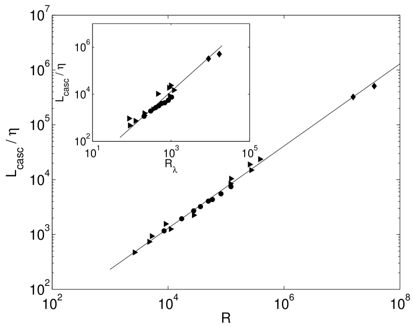
Figure 4: The dependence on the Reynolds number of the ratio of the cascade length $L_{\mathrm{casc}}$ to the Kolmogorov scale $\eta$. The a-, w- and h-records are represented by diamonds, circles and triangles, respectively. In the main graph, the straight line indicates a power-law scaling with exponent $3/4$, and the Reynolds number is defined as $R=u^{\prime}L_{\mathrm{casc}}/\nu$. The inset shows the same data over $R_{\lambda}$ with the straight line indicating the expected power-law scaling of $3/2$. The prefactor for the main graph is $A=1.3$, for the inset $A=0.41$.

The ratio increases with the large-scale Reynolds number $R=u^{\prime}L_{\mathrm{casc}}/\nu$ as a power-law with the exponent of $3/4$, exactly as anticipated if $L_{\mathrm{casc}}$ were proportional to the integral scale. The ratio $L_{\mathrm{casc}}/L$ is not exactly a constant for all the data (as can be seen from Table 1), but given the uncertainty in determining $L$ and the absence of any systematic trend suggests that our supposition is reasonable. This is further reinforced by the variation of $L_{\mathrm{casc}}/\eta$ with respect to $R_{\lambda}$ (see inset), which also follows the expected behavior. We should note that it is difficult to single out the helium data in this respect.

There is more to learn from fitting the finite-size parametrization (1) to the experimental two-point correlations than merely extracting the intermittency exponent and the cascade length. As revealed by a closer inspection of the asymptotic behavior as $d\to L_{\mathrm{casc}}$, see again Fig. 2, the two-point correlation of the atmospheric boundary layer and wind tunnel records approach their asymptotic value of unity from above, whereas for most of the gaseous helium jet records the curve first swings a little below unity before approaching the asymptotic value. The expression (1) is flexible enough to reproduce even this behavior. The derivation of (1) within the theory of binary random multiplicative cascade processes, which has been presented in Ref. CLE03b , also specifies the parameter

$$c=\frac{\langle\Pi^{2}\rangle\langle q_{L}q_{R}\rangle}{2\langle q_{L/R}^{2}\rangle-1}$$ (3)

in terms of cascade quantities. Normalized to $\langle\Pi\rangle=1$, $\Pi$ represents the initial energy flux density, which is fed into the cascade at the initial length scale $L_{\mathrm{casc}}$. $\langle q_{L/R}^{2}\rangle$ and $\langle q_{L}q_{R}\rangle$ are second-order moments of the bivariate probabilistic cascade generator $p(q_{L},q_{R})=p(q_{R},q_{L})$, which we assume to be symmetric. Again the normalization of the left and right random multiplicative weights is such that $\langle q_{L/R}\rangle=1$. Note, that $\log_{2}\langle q_{L/R}^{2}\rangle=\mu$ is equal to the intermittency exponent. Figure 5 shows various graphs of the two-point correlation (1) with the expression (3), where parameters $\mu$ and $L_{\mathrm{casc}}$ have been kept fixed, but $c$ has been varied in the range $0<c<1$.

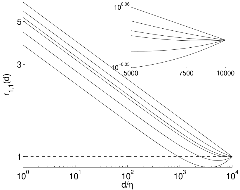
Figure 5: Two-point correlator (1) for various parameter values $c=0.6,0.7,0.8,1/(1+\mu),0.9,1$ (from left to right). The other parameters are fixed to $L_{\mathrm{casc}}/\eta=10^{4}$ and $\mu=0.20$.

We observe that for large $c$ the two-point correlation approaches its asymptotic value from above, whereas for small $c$ it swings below one before it reaches the asymptotic value from below. The transition between these two behaviors occurs at $c\approx\frac{1}{1+\mu}$. This translates to $\langle\Pi^{2}\rangle\langle q_{L}q_{R}\rangle=(2^{1+\mu}-1)/(1+\mu)$, which is $1.08$ for $\mu=0.2$ and $1.04$ for $\mu=0.1$. Hence, we are tempted to conclude that for the air data the fluctuation of the initial energy flux density fed into the inertial-range cascade at the upper length scale is somewhat larger than for the helium jet data; this appears to be plausible and is one difference between air and helium data. We also read this as an indication that $\langle q_{L}q_{R}\rangle<1$, which is fulfilled if the left and right multiplicative weight are anticorrelated to some extent. As has already been discussed in a different context JOU00 , this anticorrelation is a clear signature that the three-dimensional turbulent energy cascade conserves energy.

IV Concluding remarks

In summary, we state that the picture of the turbulent energy cascade is robust and again confirmed by the excellent agreement between the two-point correlation density predicted by random multiplicative cascade theory and that extracted from various experimental records. The cascade mechanism appears to be universal, although its strength, as represented by the intermittency exponent, seems to depend on the Reynolds number except when it is very high. The discrepancy between the air data on the one hand and the gaseous helium data on the other remains a puzzle (despite some possible explanations offered), and is in need of a fuller explanation.

- (1) G.K. Batchelor and A.A. Townsend, Proc. Roy. Soc. A 199, 238 (1949).
- (2) C. Meneveau and K.R. Sreenivasan, J. Fluid Mech. 224, 429 (1991).
- (3) K. R. Sreenivasan and P. Kailasnath, Phys. Fluids A5, 512 (1993).
- (4) A. Praskovsky and S. Oncley, Fluid Dyn. Res. 21, 331 (1997).
- (5) J. Cleve, M. Greiner and K.R. Sreenivasan, Europhys. Lett. 61, 756 (2003).
- (6) J. Cleve, T. Dziekan, J. Schmiegel, O.E. Barndorff-Nielsen, B.R. Pearson, K.R. Sreenivasan and M. Greiner, Preprint, arXiv:physics/0312113.
- (7) B. Dhruva, An Experimental Study of High Reynolds Number Turbulence in the Atmosphere, PhD thesis, Yale University (2000).
- (8) B.R. Pearson, P.A. Krogstad and W. van de Water, Phys. Fluids 14, 1288 (2002).
- (9) O. Chanal, B. Chebaud, B. Castaing, and B. Hébral, Eur. Phys. J. B 17, 309 (2000).
- (10) D. Aronson and L. Löfdahl, Phys. Fluids A 5, 1433 (1993).
- (11) R. A. Antonia, A. J. Chambers and B. R. Satyaprakash, Boundary-Layer Meteorology 21, 159 (1981).
- (12) R.A. Antonia, B.R. Satyaprakash and A.K.M.F. Hussain, J. Fluid Mech. 119, 55 (1982).
- (13) F. Anselmet, Y. Gagne, E. J. Hopfinger and R. A. Antonia, J. Fluid Mech. 140, 63 (1984).
- (14) V. R. Kuznetsov, A. A. Praskovsky and V.A. Sabelnikov, J. Fluid Mech. 243, 595 (1992).
- (15) J. Mi and R. A. Antonia, Phys. Rev. E 64, 026302 (2001).
- (16) V. Emsellem, D. Lohse, P. Tabeling, L. Kadanoff and J. Wang, Phys. Rev. E 55, 2672 (1997).
- (17) K.R. Sreenivasan and R.A. Antonia, Annu. Rev. Fluid Mech. 29, 435 (1997).
- (18) A. Gylfason, S. Ayyalasomayajulu and Z. Warhaft, J. Fluid. Mech. 501, xxx (2003).
- (19) B. Jouault, M. Greiner and P. Lipa, Physica D136, 125 (2000).