Counterposed phase velocity and energy–transport velocity vectors in a dielectric–magnetic uniaxial medium
Akhlesh Lakhtakia111Corresponding Author. Tel: +1 814 863 4319; Fax: +1 814 865 9974;
E–mail: AXL4@psu.edu
Computational & Theoretical Materials Sciences Group (CATMAS)
Department of Engineering Science & Mechanics
Pennsylvania State University, University Park, PA 16802–6812, USA
Martin W. McCall
Department of Physics, Imperial College London
Prince Consort Road, London SW7 2BZ, UK
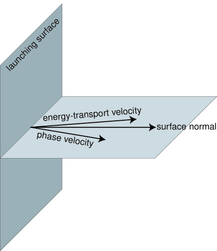
Abstract: When a plane wave is launched from a plane surface in a linear, homogenous, dielectric–magnetic, uniaxial medium, we show that its phase velocity and the energy–transport velocity vectors can be counterposed (i.e., lie on different sides of the surface normal) under certain circumstances.
Keywords: Anisotropy; Energy–transport velocity; Phase velocity;
1 Introduction
In any linear homogeneous medium, two distinct plane waves can propagate in any direction (except in very rare circumstances [1, 2], which are ignored here). With each plane wave are associated a phase velocity vector and an energy–transport velocity vector [3]. These two vectors are parallel to each other in isotropic mediums, but not in anisotropic mediums.
While examining a recently reported experimental result [4], we came across the following question: If a plane wave is launched from an infinite plane — possibly, either by reflection or refraction — into a linear, homogeneous, anisotropic medium, can the phase velocity and the energy–transport velocity vectors be counterposed (i.e., lie on different sides of the surface normal), as shown in Figure 1? Although we suspected an affirmative answer to the question, we were unable to find any treatment of the question in standard textbooks. Therefore, we undertook an investigation, the results of which are reported here.
2 Analysis
Let us consider a dielectric–magnetic uniaxial medium whose relative permittivity and relative permeability dyadics are denoted by
| (1) | |||
| (2) |
respectively, where is the identity dyadic and is a unit vector parallel to the distinguished axis of the medium.
In this medium, two distinct plane waves can propagate in any given direction, as detailed elsewhere [5]. The wavenumbers of the two plane waves are obtained as
| (3) | |||
| (4) |
where is a unit vector denoting the direction of propagation while is the free–space wavenumber. The electric and magnetic field phasors associated with the two plane waves are known, their expressions not being needed for the present purposes.
But we do need expressions for the phase velocity and the energy–transport velocity vectors. With the assumption that the imaginary parts of and are negligibly small, we obtain [5]
| (5) |
for the phase velocity vectors, and
| (6) |
for the energy–transport velocity vectors of the two plane waves, with denoting the speed of light in free space. Note that are co–parallel with the respective time–averaged Poynting vectors; and they are also co–parallel with the respective group velocity vectors in the absence of dispersion [3, Sec. 3.6].
Let us now suppose that a plane wave is launched into the half–space from the plane . We say that the phase velocity vector and the energy–transport velocity vector of the -th plane wave, (), are counterposed if the two vectors are pointed on the opposite sides of the axis.
Without loss of generality, we set
| (7) |
where and are unit cartesian vectors, while the angles and . Then, the expressions
| (8) | |||||
and
| (9) | |||||
emerge from (6).
Let us define angles , (), through the relation ; hence,
| (10) |
where the degree of uniaxiality
| (11) |
The counterposition condition then amounts to
| (12) |
Alternatively, the two velocity vectors of the -th plane wave are counterposed if when .
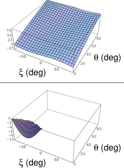
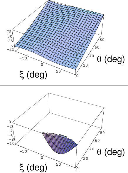
Figure 2 shows computed values of for , when the degree of uniaxiality is positive (i.e., for , and for ). Figure 3 shows the computed values for negative uniaxiality (i.e., for , and for ). The latter figure can, in fact, be deduced from Figure 2 via the substitution , but has been included for completeness. Quite clearly, a wide –range exists for very small angles for which the counterposition condition is satisfied. As increases, the –range for counterposition diminishes and eventually vanishes. The higher the degree of uniaxiality in magnitude, the larger is the portion of the space wherein the counterposition condition is satisfied.
3 Conclusion
When a plane wave is launched from a plane surface — possibly by refraction or reflection — in a linear, homogenous, dielectric–magnetic, uniaxial medium, we have shown here that its phase velocity and the energy–transport velocity vectors may be counterposed. An excellent experimental example has been furnished by Zhang et al. [4].
References
- [1] Gerardin J, Lakhtakia A: Conditions for Voigt wave propagation in linear, homogeneous, dielectric mediums. Optik 112 (2001) 493–495.
- [2] Berry MV, Dennis MR: The optical singularities of birefringent dichroic chiral crystals. Proc. R. Soc. Lond. A 459 (2003) 1261–1292.
- [3] Chen HC: Theory of Electromagnetic Waves. McGraw–Hill, New York, USA 1983.
- [4] Zhang Y, Fluegel B, Mascarenhas A: Total negative refraction in real crystals for ballistic electrons and light. Phys. Rev. Lett. 91 (2003) 157404.
- [5] Lakhtakia A, Varadan VK, Varadan VV: Plane waves and canonical sources in a gyroelectromagnetic uniaxial medium. Int. J. Electron. 71 (1991) 853–861.