Spatial Coherence of Synchrotron Radiation

Abstract

Theory and measurement of spatial coherence of synchrotron radiation beams are briefly reviewed. Emphasis is given to simple relationships between electron beam characteristics and far field properties of the light beam.

Introduction

Synchrotron Radiation (SR)handbook ; esrfcd ; wordscientific has been widely used since the 80’s as a tool for many applications of UV, soft X rays and hard X rays in condensed matter physics, chemistry and biology. The evolution of SR sources towards higher brightness has led to the design of low-emittance electron storage rings (emittance is the product of beam size and divergence), and the development of special source magnetic structures, as undulators. This means that more and more photons are available on a narrow bandwidth and on a small collimated beam; in other words there is the possibility of getting a high power in a coherent beam. In most applications, a monochromator is used, and the temporal coherence of the light is given by the monochromator bandwidth. With smaller and smaller sources, even without the use of collimators, the spatial coherence of the light has become appreciable, first in the UV and soft X ray range, and then also with hard X rays. This has made possible new or improved experiments in interferometry, microscopy, holography, correlation spectroscopy, etc. attwood ; cornacchia ; attwood_pt ; attwoodbook ; kondratenko ; alferov ; tang . In view of these recent possibilities and applications, it is useful to review some basic concepts about spatial coherence of SR, and its measurement and applications. In particular we show how the spatial coherence properties of the radiation in the far field can be calculated with simple operations from the single-electron amplitude and the electron beam angular and position spreads. The gaussian approximation will be studied in detail for a discussion of the properties of the far field mutual coherence and the estimate of the coherence widths, and the comparison with the VanCittert-Zernike limit.

I Spatial Coherence (SC)

First let us remind some concepts and define some symbols about SC of a quasi-monochromatic field in general. If we have paraxial propagation of a random electromagnetic field $f(\bm{\mathrm{p}})$ (where $\bm{\mathrm{p}}=(x,y)$ is a point in the transverse plane) along a direction $z$, the filed $f(\bm{\mathrm{p}})n$ at $z=0$ propagates in the Fresnel approximation

$$f_{z}(\bm{\mathrm{p}})=\frac{1}{(\lambda z)^{2}}\int{f_{0}(\bm{\mathrm{p}}_{0})\,e^{-\frac{ik}{z}(\bm{\mathrm{p}}-\bm{\mathrm{p}}_{0})^{2}}\,d^{2}\bm{\mathrm{p}}}\,,$$ (1)

and in the Far Field (FF) (Fraunhofer region), where most observations are done, we have

$$\tilde{f}(\bm{\mathrm{k}})=\mathrm{F}_{\bm{\mathrm{p}}\rightarrow\bm{\mathrm{k}}}f(\bm{\mathrm{p}})=\frac{1}{\sqrt{2\pi}}\int{f(\bm{\mathrm{p}})\,e^{i\bm{\mathrm{k}}\cdot\bm{\mathrm{p}}}\,d^{2}\bm{\mathrm{p}}}$$ (2)

where we have dropped the index $0$ and indicated with $F_{\bm{\mathrm{p}}\rightarrow\bm{\mathrm{k}}}$ the Fourier transform operator from $\bm{\mathrm{p}}$ to $\bm{\mathrm{k}}$ domain. Here we use as a variable the transverse component of the wavevector $\bm{\mathrm{k}}=(k_{x},k_{y})$, the observation angle is then

$$\theta=\bm{\mathrm{k}}\frac{\lambda}{2\pi}\,,$$ (3)

According to eq. (2), angles are expressed in terms of reciprocal space coordinates, as is natural in diffraction optics.

“Second-order” statistical properties of the field are described by the “mutual intensity” (m.i.) (see goodman ), i.e. the ensemble average of the products of fields at two points.

It is convenient to express the m.i. as a function of the average and difference coordinates: $\bm{\mathrm{p}}_{1}=\bm{\mathrm{p}}-\Delta\bm{\mathrm{p}}/2$, $\bm{\mathrm{p}}_{2}=\bm{\mathrm{p}}+\Delta\bm{\mathrm{p}}/2$ and, in reciprocal space, $\bm{\mathrm{k}}_{1}=\bm{\mathrm{k}}-\Delta\bm{\mathrm{k}}/2$, $\bm{\mathrm{k}}_{2}=\bm{\mathrm{k}}+\Delta\bm{\mathrm{k}}/2$

$$\mathrm{M}f(\bm{\mathrm{p}},\Delta\bm{\mathrm{p}})=\langle f^{*}(\bm{\mathrm{p}}-\Delta\bm{\mathrm{p}}/2)f(\bm{\mathrm{p}}+\Delta\bm{\mathrm{p}}/2\rangle$$ (4)

For simplicity we will also use these symbols:

$$\mathrm{I}f(\bm{\mathrm{p}})=\mathrm{M}f(\bm{\mathrm{p}},0)$$

the intensity and

$$\mathrm{C}f(\Delta\bm{\mathrm{p}})=\int Mf(\bm{\mathrm{p}},\Delta\bm{\mathrm{p}})d^{2}\bm{\mathrm{p}}$$

the (integrated) autocorrelation. The degree of (spatial) coherence is defined as

$$\mu f(\bm{\mathrm{p}},\Delta\bm{\mathrm{p}})\equiv\mathrm{M}f(\bm{\mathrm{p}},\Delta\bm{\mathrm{p}})/\sqrt{I(\bm{\mathrm{p}}-\Delta\bm{\mathrm{p}}/2)I(\bm{\mathrm{p}}+\Delta\bm{\mathrm{p}}/2)}$$ (5)

The Fresnel propagation of the m.i. can be expressed as:

$$\mathrm{M}f_{z}(\bar{\bm{\mathrm{p}}},\Delta\bar{\bm{\mathrm{p}}})=\frac{1}{(\lambda z)^{2}}\int\mathrm{M}f_{0}(\bm{\mathrm{p}},\Delta\bm{\mathrm{p}})e^{i\frac{k}{z}(\bar{\bm{\mathrm{p}}}-\bm{\mathrm{p}})(\Delta\bar{\bm{\mathrm{p}}}-\Delta\bm{\mathrm{p}})}d^{2}\bm{\mathrm{p}}\,d^{2}\Delta\bm{\mathrm{p}}$$ (6)

and in the FF

$$\left\langle\tilde{f}(\bm{\mathrm{k}}-\tfrac{\Delta\bm{\mathrm{k}}}{2})\tilde{f}(\bm{\mathrm{k}}+\tfrac{\Delta\bm{\mathrm{k}}}{2})\right\rangle=\int\mathrm{M}f(\bm{\mathrm{p}},\tfrac{\Delta\bm{\mathrm{p}}}{2})e^{i\bm{\mathrm{p}}\cdot\Delta\bm{\mathrm{k}}+\bm{\mathrm{k}}\cdot\Delta\bm{\mathrm{p}}}d^{2}\bm{\mathrm{p}}\,d^{2}\Delta\bm{\mathrm{p}}$$ (7)

or, with our simplified notation,

$$\mathrm{M}\tilde{f}(k,\Delta k)=\mathrm{F}_{\bm{\mathrm{p}}\rightarrow\Delta\bm{\mathrm{k}}}F_{\Delta\bm{\mathrm{p}}\rightarrow\bm{\mathrm{k}}}\mathrm{M}f(\bm{\mathrm{p}},\Delta\bm{\mathrm{p}})\,.$$

From this, two useful reciprocity relations connecting source and FF intensity/coherence properties can be derived friberg ; coissoncern :

$$\mathrm{FC}f(\bm{\mathrm{k}})=\mathrm{IF}f(\bm{\mathrm{k}})$$ (8)

$$\mathrm{FI}f(\Delta\bm{\mathrm{k}})=\mathrm{C}Ff(\Delta\bm{\mathrm{k}})$$ (9)

and reciprocal ones interchanging source and FF. Properties of non-stationary random functions can also be described by the Wigner function (WF) (which is a photon number distribution in phase space, if divided by $\hbar\omega$) kim ; coissonspie86 ; walther :

$$\mathrm{W}f(\bm{\mathrm{p}},\bm{\mathrm{k}}) = \int\left\langle f(\bm{\mathrm{p}}-\Delta\bm{\mathrm{p}}/2)f^{*}(\bm{\mathrm{p}}+\Delta\bm{\mathrm{p}}/2)\right\rangle e^{i\Delta\bm{\mathrm{p}}\cdot\bm{\mathrm{k}}}d^{2}\Delta\bm{\mathrm{p}}$$ (10)

$$= \int\left\langle\tilde{f}(\bm{\mathrm{k}}-\Delta\bm{\mathrm{k}}/2)\tilde{f}^{*}(\bm{\mathrm{k}}+\bm{\mathrm{k}}/2)\right\rangle e^{i\Delta\bm{\mathrm{k}}\cdot\bm{\mathrm{p}}}d^{2}\Delta\bm{\mathrm{k}}$$

In fact from the definition we see that Fourier-transforming the WF with respect to k one gets the m.i. of f(x), while transforming with respect to x gives the m.i. of $\tilde{f}(k)$. We also remind that the intensity at the object plane $If=\int Wfdk$ and in the far field $I\tilde{f}=\int Wfdx$.

An equivalent description, with essentially the same characteristics, could be obtained with the Ambiguity function papoulis:josa

$$Af(\Delta\bm{\mathrm{p}},\Delta\bm{\mathrm{k}})=\int<f(\bm{\mathrm{p}}-\Delta\bm{\mathrm{p}}/2)f^{*}(\bm{\mathrm{p}}+\Delta\bm{\mathrm{p}}/2)>e^{i\bm{\mathrm{p}}\cdot\Delta\bm{\mathrm{k}}}\,d^{2}\bm{\mathrm{p}}$$ (11)

Both Wigner and Ambiguity functions are real (almost always positive) functions and can be considered as a phase space energy density: notice that this phase space area is dimensionless. $Wf$ propagates in the same way of the “radiance” (or “brightness”) of geometrical optics:

$$Wf_{z}(\bm{\mathrm{p}},\bm{\mathrm{k}})=Wf_{0}(\bm{\mathrm{p}}-\frac{\bm{\mathrm{k}}}{k}z,\bm{\mathrm{k}})\,,$$ (12)

and the same for $Af_{z}(\Delta\bm{\mathrm{p}},\Delta\bm{\mathrm{k}})$.

I.1 Gaussian approximation

A gaussian model (also called a gaussian Schell modelmandelandwolf ) of a partially coherent field has a radiance which has a 4-D gaussian distribution in phase space. From now on let us for simplicity consider one transverse dimension, say x (and $k_{x}$ will be called k for short): we have then [ $\mathrm{W}f$ or $\mathrm{A}f$ ] of the form (using our previous symbols):

$$\mathrm{W}f(x,k)=N_{1}\exp\left(-\tfrac{1}{2}\tfrac{x^{2}}{\sigma_{I}^{2}}\right)\exp\left(-\tfrac{1}{2}\tfrac{k^{2}}{s_{I}^{2}}\right)$$ (13)

the $\mathrm{M}I$ is then

$$Mf(x,\Delta x)=N_{2}\exp\left(-\tfrac{1}{2}\tfrac{x^{2}}{\sigma_{I}^{2}}\right)\exp\left(-\tfrac{1}{2}\tfrac{\Delta x^{2}}{\sigma_{M}^{2}}\right)$$ (14)

where

$$\sigma_{M}=\frac{1}{s_{I}}$$ (15)

(in agreement with eq. 8), if we define $\sigma_{M}$ as the width of $Cf(\Delta x)$. Here we have indicated with N the normalisation constants)

This MI clearly satisfies separability between x and $\Delta x$ (Walther’s condition walther ). When $\sigma_{M}\ll\sigma_{I}$ we have the “quasi-homogeneous” approximation ($Mf(x,\Delta x)=If(x)\mu f(\Delta x)$), and the factor function of $x$ has the meaning of the intensity carter .

We easily see that this model satisfies the Schell condition (that’s why it is also called “gaussian Schell” model) that the degree of coherence depends only on the separation between two points $\Delta x$) : eq. 14 can be written:

$$\mathrm{M}f(x,\Delta x)=N\exp\left\{-\tfrac{1}{2}\frac{(x-\Delta x/2)^{2}}{2\sigma_{I}^{2}}\right\}\exp\left\{-\tfrac{1}{2}\frac{(x+\Delta x/2)^{2}}{2\sigma_{I}^{2}}\right\}\exp\left\{-\tfrac{1}{2}\frac{\Delta x^{2}}{\sigma_{\mu}^{2}}\right\}$$ (16)

where

$$\frac{1}{\sigma_{\mu}^{2}}=\frac{1}{\sigma_{M}^{2}}-\frac{1}{4\sigma_{I}^{2}}$$ (17)

In particular, we see that for a perfectly coherent gaussian beam, $\sigma_{M}=2\sigma_{I}$. The Schell and Walther conditions are satisfied simultaneously only for a plane wave and gaussian wave: writing the two conditions,

$$\left[\mathrm{I}f\left(x+\tfrac{\Delta x}{2}\right)\mathrm{I}f\left(x-\tfrac{\Delta x}{2}\right)\right]^{\frac{1}{2}}\mu f(\Delta x)=\mathrm{M}f\left(x,\Delta x\right)=\mathrm{I}f\left(x\right)\mathrm{m}f(\Delta x)$$ (18)

If we apply the logarithm and call $h(\Delta x)=\log[\mu f(\Delta x)/\mathrm{m}f(\Delta x)]$, $L(x)=\log[\mathrm{I}f(x)]$ Eq. 18 becomes:

$$2L(x)-L\left(x+\tfrac{\Delta x}{2}\right)-L\left(x-\tfrac{\Delta x}{2}\right)=2h(\Delta x)$$

By Taylor expanding $L$ we see that in order for the left term to be dependent only on $\Delta x$, terms higher than 2 must be 0, i.e. a Gaussian, exponential or flat intensity only.

II Mutual intensity of Synchrotron Radiation

A characteristic of SR is that it is the random superposition of a large number of rather collimated elementary waves emitted by each electron of the beam kim ; coissonspie86 ; coisson:jsr . Let us call $\tilde{a}(\bm{\mathrm{k}})$ the well-known far-field amplitude (or square root of the intensity) emitted by a single electron. It can be seen as the FT of the amplitude at the source $a(\bm{\mathrm{p}})$, which of course is not a Dirac delta because of the diffraction corresponding to the limited angular aperture (and this is a limit to the possibility of localizing an electron by observing or imaging the emitted SR). The electron beam is characterized by a transverse spatial distribution g(p) and an angular distribution $\gamma(\bm{\mathrm{k}})$, which are to a good approximation both gaussian. The ratio of the beam size and angular aperture is called the beta function and it is known from the machine physics. Usually the source is in a place where position and angular distribution are uncorrelated; otherwise it is possible to define an effective source position at the “waist” point where the two distibutions are uncorrelated. The “waist” points may be different for the vertical and the horizontal distributions.

We will consider for simplicity one transverse coordinate, say $x$ and $k$. The superposition of all elementary contributions can be best described in phase space, where the Wigner function (or Ambiguity function) can be obtained by a convolution of the two distributions (electron, and single-electron light) kim ; coissonspie86 .

$$\mathrm{W}f(x,k)=g(x)\gamma(k)**\mathrm{W}a(x,k)$$ (19)

where $**$ indicated the convolution with respect to both variables. The source and FF mutual intensities are then coisson:ao95 :

$$\mathrm{M}f(x,\Delta x)=\tilde{\gamma}(\Delta x)[g(x)*\mathrm{M}a(x,\Delta x)]$$ (20)

and

$$\mathrm{M}\tilde{f}(k,\Delta k)=\tilde{g}(\Delta k)[\gamma(k)*\mathrm{M}\tilde{a}(k,\Delta k)]$$ (21)

In particular, for the FF intensity:

$$\mathrm{I}\tilde{f}(k)=\gamma(k)*\mathrm{I}\tilde{a}(k)$$ (22)

In order to give estimates of sizes and correlation distances of SR, it is useful to use a gaussian approximation for the SR distributions $a(x)$ and $\tilde{a}(k)$. Actually they are not gaussians, but this approximation is rather good for two reasons: $g(x)$ and $\gamma(k)$ being gaussians, the convolution is close to a gaussian, except on the tails (as $a(x)$ has long tails), and the part that is used is just the central one.

With this gaussian approximation, the source and FF are characterised by 6 gaussian widths.

Let us call $\sigma_{I}$ the characteristic width of the intensity (so that $I(x)=\exp(-x^{2}/2\sigma^{2})$) at the source, and $s_{I}$ the FF intensity width. The M.I. of the source is given by eq. 14

As we have seen (eq. 14), the degree of coherence $\mu f(x)$ has a width which is related to the other two widths by:

$$\frac{1}{\sigma_{\mu}^{2}}=\frac{1}{\sigma_{M}^{2}}-\frac{1}{4\sigma_{I}^{2}}$$ (23)

And analogously, if we use $s$ for the FF widths:

$$\frac{1}{s_{\mu}^{2}}=\frac{1}{s_{M}^{2}}-\frac{1}{4s_{I}^{2}}$$ (24)

On the other hand, if we apply the reciprocity relations (Eq. 8, 9 ) to the gaussian case, we have:

$$s_{M}=\frac{1}{\sigma_{I}}\,,\text{ and }s_{I}=\frac{1}{\sigma_{M}}$$ (25)

This is illustrated in fig 1

Figure 1: Illustration of the source - far field reciprocity relations (eq. 25), note that in the gaussian case the ratio between beam width and coherence width is the same in the near field and far field (as well as in all sections in between coisson:jsr )

We want now to correlate these widths with the electron and SR characteristics. We approximate the single-electron FF amplitude with

$$\tilde{a}(k)=\exp\left(-\frac{k^{2}}{4\rho^{2}}\right)$$ (26)

In this way we have defined $\rho$ as the gaussian width of the FF intensity. The angular width $\rho$ is of the order of the relativistic factor of the electrons (multiplied by $2\pi/\lambda$, in our reciprocal space units) alferov ; coisson:oe ; coisson:ao88

If we also apply to the gaussian case eqs. 19, we get

$$s_{I}^{2}=s_{e}^{2}+\rho^{2}\text{, and }\sigma_{I}^{2}=\sigma_{e}^{2}+1/4\rho^{2}$$ (27)

Putting together these relations, we can eventually determine the intensity and coherence properties of the FF as a function of electron beam (and single-electron radiation) data:

$$s_{I}=(s_{e}^{2}+\rho^{2})^{1/2}\,,\,s_{M}=(\sigma_{e}^{2}+1/4\rho^{2})^{-1/2}$$

$$s_{\mu}=\left(\sigma_{e}^{2}+\frac{1}{4\rho^{2}}-\frac{1}{4(s_{e}^{2}+\rho^{2})}\right)^{-1/2}$$ (28)

In the perfectly coherent limit ($s_{e}<<1/\rho$ and $s_{e}<<\rho$) we have $s_{\mu}=\infty$, $s_{I}=\rho$ and $s_{M}=\rho$. The quasi-homogeneous case is when $s_{e}>>\rho$ and $\sigma_{e}>>1/\rho$: in this case

$$s_{\mu}=(\sigma_{e}^{2}+1/4\rho^{2})^{-1/2}\simeq 1/\sigma_{e}$$ (29)

This result coincides with the VanCittert-Zernike theorem, valid in the limit of a completely incoherent source. In general, however (for a rather coherent beam, that is a beam produced by an electron beam with small $\sigma_{e}$ and $s_{e}$), the VanCittert-Zernike theorem needs a correction coisson:ao95 .

It may also be of interest to know the resolution for imaging the source on the basis of FF intensity and coherence measurements. In principle, we can get both $\sigma_{e}$ and $s_{e}$ by measuring $s_{I}$ and $s_{M}$ or $s_{\mu}$: from the previous equations we see that from eq 27 we get

$$s_{e}^{2} = s_{I}^{2}-\rho^{2}\,,$$

$$\sigma_{e}^{2} = 1/s_{M}^{2}-1/4\rho^{2}\,.$$ (30)

However in practice the low precision of correlation measurement with the unfavorable propagation of errors, makes the method usable only if $4\rho^{2}/s_{M}^{2}-1$ and $s_{I}^{2}/\rho^{2}-1$ are not much smaller than one, i.e. the beam is not much smaller than the diffraction limit).

In these remarks we have considered always a quasi-monochromatic component of the field; in other words we imagine the light to be filtered before by a monochromator. It may be worthwhile to mention that SR, and in particular the radiation from undulators, is not “cross-spectrally pure” as defined by Mandel mandel , as the spectrum depends on angle, and then the spatial coherence and spectral characteristics cannot be separated, a subject that has not yet been analysed in the literature.

III Effects of quality of optical elements.

In recent machines where spatial coherence becomes appreciable over a fraction of the photon beam width, or in other words is very well collimated (near the diffraction limit), the effect of imperfection of optical elements, as mirrors coissonreport ; wang or Berillium windows snigirev:nima strongly influences the beam quality. For mirrors, if the rms slope error is $\varsigma$, this must be compared with $\theta_{coh}=\lambda s_{\mu}/2\pi$: in order to have small distortions we should have $\varsigma<<\theta_{coh}$ For windows, a uniform illumination will become non-uniform, with a contrast

$$C=2\pi h/\lambda(n-1)$$

.

Some authors have called this degradation of beam quality a “reduction of coherence” snigirev:nima ; snigirev:rsi . Actually this is not precise nugent:optexp , as the speckle-like field produced by a random deflection from a rough surface (or refraction from a rough window) is still capable of producing interference fringes in a Young experiment if the original wave was spatially coherent. In fact, the optical path (as a function of x,y) is fixed in time, it is a single realization of a random function, in other words a deterministic function (although not known in detail). We have to distinguish averages in time from averages over an ensemble of optical elements with similar statistical properties. The measure of correlation distance is given by $\sigma_{\mu}$ or $s_{\mu}$, not by $\sigma_{M}$ or $s_{M}$, as the latter ones maybe short, for example, in a perfectly coherent light with strong and rapid spatial variations of intensity.

In other words, coherent light stays coherent, even after passing through a random media. The photons in a coherent volume in phase space never mix with others as a consequence of the Liouville theorem. However when we perform a measurement, we normally measure projections (intensity) or slices (interferometry) in phase space. In the case of a Young’s slits experiment for example, the two slits act as slices in the phase space, the beams diffracted from the slits have lost directionality, and different volumes in phase space are therefore mixed. In a intensity interferometry experiment, we integrate the phase space distribution over the angles vartanyants:optcom .

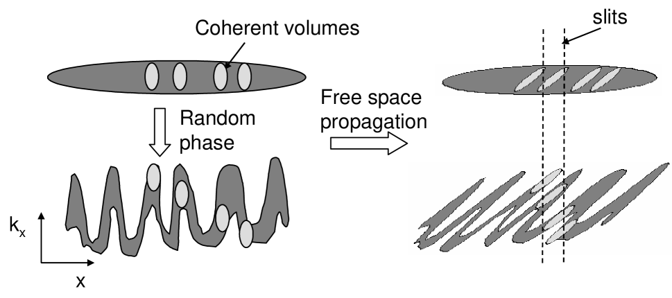
Figure 2: propagation of the wigner function: (top) a gauss-shell beam propagates in free space, and a coherent volume is selected by two slits. (bottom) the same beam after passing through a random phase object

IV Measurements

The first soft x-ray interferometric measurements with synchrotron radiation were performed by Polack et al polak using two mirrors with an angle between them of 2.25 arcmin at 6⁰ grazing angle. Coherence measurements using Young slits have been performed by many groups in the soft X-ray range takayama ; xu ; chang ; paterson . Takayama used a young-slit experiment to characterize the emittance of the electron beam takayama1 .

In the hard x-ray the first interferometric measurement of the beam coherence was performed using two mirrors at grazing incidence acting as slits fezzaa ; marchesini:oe96 ; marchesini (Fig. 3). Normal slits have also been applied leitenberger .

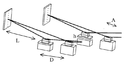
Figure 3: experimental setup used to perform hard x-ray interferometric characterization of the coherence. By moving $D$ or changing the angle of incidence, or the height $h$ of one mirror one can study the vertical coherence, while by tilting one mirror it is possible to study the horizontal coherence fezzaa .

Other measurements of coherence have been performed by diffracting x-rays from a wire snigireva ; kohnprl , using Talbot effect cloetens , a mask of coded apertures called a uniformly redundant array (URA) lin:prl . Other techniques include using nuclear resonance from a rotating disk and measuring the spatial coherence in the time domain (the rotating disk acts as a ’prism’ of increasing angle) baron , and intensity interferometry yabashi:2001 . The latter has been used to measure the spatial as well as longitudinal coherence yabashi:2002 and characterize the 3 dimensional x-ray pulse widths. Variation of the visibility of a speckle pattern can also be used as an indication of the coherence width abernathy .

- (1) see for ex. Handbook on Synchrotron Radiation, E. E. Koch, Ed., Vol.1-4, North Holland, Amsterdam (vol.1 in 1983).
- (2) Synchrotron Light CD-ROM, ISBN 3-540-14888-4, IMEDIASoft/Springer-Verlag/ESRF, 2000
- (3) Series on Synchrotron Radiation Techniques and Applications, Word Scientific, Singapore 2000 Volume 1: Synchrotron Radiation Sources - A Primer, edited by Herman Winick Volume 5 Synchrotron Radiation Theory and Its Development, edited by Vladimir A Bordovitsyn Volume 6 Insertion Devices for SR and FEL by F Ciocci, G Dattoli, A Torre & A Renieri
- (4) D. Attwood, K. Halbach, K.-J. Kim, “Tunable coherent X-rays”, Cambridge University Press; (September 1999)
- (5) M. Cornacchia, H. Winick, XV Int. Conf. on High Energy Accel., Hamburg 1992. Science 228,1265-72 (1985).
- (6) D. Attwood, “New opportunities at soft X-ray wavelengths”,Phys. Today, August 1992, p.24-31.
- (7) “Soft X-Rays and Extreme Ultraviolet Radiation : Principles and Applications”, D. Atwood, Cambridge University Press, (Cambridge 1999).
- (8) A. M. Kondratenko, A. N. Skrinsky “Use of radiation of electron storage rings in X-ray holography of objects”, Opt. Spektrosk. 42, 338-344 (1975); Engl. transl. in: Opt. Spectrosc. 42, 189-192 (1977).
- (9) D. F. Alferov, Yu. A. Bashmakov, E. G. Bessonov, “Theory of undulator radiation”, Zh. Tech. Fiz. 48, 1592-1597 and 1598-1606 (1978); Engl. transl. in: Sov. Phys. Tech. Phys. 23, 902-904 and 905-909 (1978).
- (10) E.Tang, P.Zhu, M.Cui, ”Coherence mode of SR”, Acta Optica Sinica 18, 1645 (1998).
- (11) J. W. Goodman, Statistical Optics, ch. 5, J.Wiley, NY 1985.
- (12) A. Friberg, E. Wolf, “Reciprocity relations with partially coherent sources”, Opt. Acta 30, 1417-1435(1983).
- (13) R. Coïsson, “Source and far field coherence functions”, Note SPS/ABM/RC 81-11, CERN, Geneva 1981.
- (14) K.-J. Kim, “A new formulation of synchrotron radiation optics using the Wigner distribution”, Proc SPIE 582, 2-9 (1986).
- (15) R. Coïsson, R. P. Walker, “Phase space distribution of brilliance of undulator sources” Proc. SPIE 582, 24-29 (1986).
- (16) A. Walther, “Radiometry and coherence”, J. Opt. Soc. Am. 58,1256-59 (1968).
- (17) W. H. Carter, E. Wolf, “Coherence and radiometry with quasihomogeneous planar sources”, J. Opt. Soc. Am. 67,785 (1977);
- (18) A. Papoulis, “Ambiguity function in Fourier optics”, J. Opt. Soc. Am.64, 779-788 (1974).
- (19) L.Mandel and E.Wolf, Optical Coherence and Quantum Optics, (Cambridge University Press, Cambridge, 1995)
- (20) R. Coïsson, S. Marchesini, Gauss-Shell sources as model for Synchrotron Radiation, Journal of Synchrotron Radiation 4(5), 1997, 263-266.
- (21) R. Coïsson, “Spatial coherence of synchrotron radiation”, Appl. Opt. 34, 904-8 (1995)
- (22) R. Coïsson, “Effective phase space widths of undulator radiation”, Opt. Eng. 27, 250-52 (1988).
- (23) R. Coïsson, B.Diviacco, “Practical estimates of peak flux and brilliance of undulator radiation on even harmonics”, Appl. Opt. 27,1376-7 (1988).
- (24) L. Mandel, “Concept of cross-spectral purity in coherence theory”, J. Opt. Soc. Am. 51, 1342 (1961).
- (25) R.Coïsson, “Estimation of the effect of slope errors on soft X-ray optics”, report TSRP-IUS-1-87, Trieste 1987.
- (26) Y. Wang et al., “Effect of surface roughness of optical elements on spatial coherence of X-ray beams from third generation SR sources”, Acta Optica Sinica 20, 553-559 (2000)
- (27) A. Snigirev, I. Snigireva, V. G. Kohn, S. M. Kuznetsov, “On the requirements to the instrumentation for the new generation of the synchrotron sources: berillium windows”, Nucl. Instrum.& Meth. A, 370, pp 634-640 (1996) On the requirements to the instrumentation for the new generation of the radiation sources. Beryllium windows
- (28) A. Snigirev, I. Snigereva, V. Kohn, S. Kuznetsov, I. Schelokov, “On the possibilities of x-ray phase contrast microimaging by coherent high-energy synchrotron radiation,” Rev. Sci. Instrum. 66, 5846-5492 (1995).
- (29) K. A. Nugent, C. Q. Tran, and A. Roberts, “Coherence transport through imperfect x-ray optical systems”, Optics Express Vol. 11, No. 19, pp. 2323 - 2328 (2003).
- (30) I.A. Vartanyants and I.K. Robinson, Origins of decoherence in coherent X-ray diffraction experiments, Opt. Commun. 222, 29-50 (2003).
- (31) F. Polack, D. Joyeux, J. Svatos, and D. Phalippou, “Applications of wavefront division interferometers in soft x rays,” Rev. Sci. Instrum. 66, 2180 (1995).
- (32) Takayama Y, Tai RZ, Hatano T, et al. Measurement of the coherence of synchrotron radiation J Synchrotron Radiat 5: 456-458 Part 3 MAY 1 1998
- (33) X.Xu et al., ”Experimental investigation of spatial coherence for soft X-ray beam in Hefei national SR facility”, Acta Photonica Sinica 29, 29 (2000)
- (34) C. Chang et al., ”Spatial coherence characterization of undulator radiation”, Optics Comm. 182, 23-34 (2000)]
- (35) Paterson D, Allman BE, McMahon PJ, et al. Spatial coherence measurement of X-ray undulator radiation Opt Commun 195 (1-4): 79-84 Aug 1 2001
- (36) Y. Takayama, T. Hatano, T. Miyahara and W. Okamoto “Relationship Between Spatial Coherence of Synchrotron Radiation and Emittance”, J. Synchrotron Rad. 5, 1187(1998).
- (37) S. Marchesini, R. Coïsson, “Two-dimensional coherence measurements with Fresnel mirrors”, Opt. Eng. 35, 3597 (1996)
- (38) K. Fezzaa, F. Comin, S. Marchesini, R. Coïsson and M. Belakhovsky, X-ray Interferometry using 2 coherent beams from Fresnel mirrors, Journal of X-rays Science and Technology 7, 12-23, (1997)
- (39) S. Marchesini, K. Fezzaa, M. Belakhovsky M, R. Coïsson X-ray interferometry of surfaces with Fresnel mirrors, Appl. Optics 39 (10) 1633-1636, 2000.
- (40) Leitenberger W, Kuznetsov SM, Snigirev A “Interferometric measurements with hard X-rays using a double slit” Opt Commun 191 (1-2): 91-96 May 1 2001
- (41) Kohn V, Snigireva I, Snigirev A “Direct measurement of transverse coherence length of hard x rays from interference fringes”, Phys. Rev. Lett. 85 (13): 2745 (2000)
- (42) Snigireva I, Kohn V, Snigirev A Interferometric techniques for characterization of coherence of high-energy synchrotron X-rays Nucl Instrum Meth A 467: 925-928 Part 2 Jul 21 2001
- (43) Cloetens P, Guigay JP, DeMartino C, et al. Fractional Talbot imaging of phase gratings with hard x rays Opt Lett 22 (14): 1059-1061 JUL 15 1997
- (44) J. J. A. Lin, D. Paterson, A. G. Peele, P. J. McMahon, C. T. Chantler, and K. A. Nugent “Measurement of the Spatial Coherence Function of Undulator Radiation using a Phase Mask”, Phys. Rev. Lett. 90, 074801 (2003)
- (45) A. Q. R. Baron “Transverse coherence in nuclear resonant scattering of synchrotron radiation” Hyperfine Interact 123 (1-8): 667-680, 1999
- (46) M. Yabashi, K. Tamasaku, and T. Ishikawa, “Characterization of the Transverse Coherence of Hard Synchrotron Radiation by Intensity Interferometry”, Phys. Rev. Lett. 87, 140801 (2001)
- (47) M. Yabashi, K. Tamasaku, and T. Ishikawa, “Measurement of X-Ray Pulse Widths by Intensity Interferometry”, Phys. Rev. Lett. 88, 244801 (2002)
- (48) Abernathy DL, Grubel G, Brauer S, et al. Small-angle X-ray scattering using coherent undulator radiation at the ESRF J Synchrotron Radiat 5: 37-47 Part 1 JAN 1 1998
- (49) G. Grübel et al., “Scattering with coherent X-rays”, ESRF Newsletter 20, 14 (February 1994).
- (50) I.Schelokov, et al., “X-ray interferometry technique for mirror and multilayer characterisation”, SPIE vol.2805, 282-292, 1996