Evaluation of the self-energy correction to the $\boldsymbol{g}$-factor of $\boldsymbol{S}$ states in H-like ions

Abstract

A detailed description of the numerical procedure is presented for the evaluation of the one-loop self-energy correction to the $g$-factor of an electron in the $1s$ and $2s$ states in H-like ions to all orders in $Z\alpha$.

I Introduction

Recently, several high-precision experiments have been performed on the bound-electron $g$-factor in H-like carbon and oxygen by the Mainz-GSI collaboration Haeffner00 ; Verdu02 . The value actually measured in the experiment is $(g\,m/M)$, where $m$ is the electron mass, $M$ is the ion mass, and $g$ is the $g$-factor of the electron. The relative accuracy of the best experimental determination of this value Haeffner00 is $5\times 10^{-10}$, which is 4 times better than that of the accepted value for the electron mass Mohr00 . Further progress is anticipated from the experimental side, as well as extension of measurements to the higher-$Z$ region Werth01 .

The spectacular experimental results have triggered great interest to the theoretical description of the $g$-factor of a bound electron Blundell97 ; Persson97 ; Beier00 ; Czarnecki01 ; Karshenboim01 ; Karshenboim01a ; Shabaev01 ; Martynenko01 ; Glazov02 ; Beier02 ; Nefiodov02 ; Shabaev02PRL ; Yerokhin02 ; Shabaev02 ; Yan02 ; Yerokhin02CJP ; Shabaev03 . Combining experimental values with accurate theoretical predictions for the bound-electron $g$-factor resulted in an independent determination of the electron mass Beier02 ; Yerokhin02 . The current accuracy of this determination Yerokhin02 is 4 times better than that of the accepted value for the electron mass Mohr00 . For the latest compilation of various contributions to the bound-electron $g$-factor we refer the reader to Yerokhin02CJP for H-like ions and to Shabaev02 ; Shabaev03 for Li-like ions.

In the present work we give a detailed description of our calculation of the self-energy correction to the bound-electron $g$-factor for $1s$ and $2s$ states of a H-like ion. The first results of this calculation for the $1s$ state were previously published in Yerokhin02 , where they were used for the determination of the electron mass. In this paper, we extend our consideration to a higher-$Z$ region and perform calculations also for the $2s$ state, having in mind the planned extension of the experiments to Li-like systems.

Our calculation is carried out in the Feynman gauge. The relativistic units ($\hbar=c=1$) and the Heaviside charge units ($\alpha=e^{2}/4\pi$, $e<0$) are used throughout the paper. We also use the notations $p\!\!\!/=p_{\mu}\gamma^{\mu}$ and $\hat{{\bf p}}={\bf p}/|{\bf p}|$.

II Basic formulas

In this paper we will consider a bound electron in an $s$ state of a H-like ions with a spinless nucleus interacting with a static homogeneous magnetic field. The bound-electron $g$-factor is defined by

$$g=-\frac{\langle j_{a}m_{a}|\mu_{z}|j_{a}m_{a}\rangle}{\mu_{0}\,m_{a}}\,,$$ (1)

where $\mu$ is the operator of the magnetic moment of the electron, $\mu_{0}=|e|/(2m)$ is the Bohr magneton, $j_{a}$ is the total angular momentum of the electron, and $m_{a}$ is its projection. The lowest-order value for the $g$ factor can be found by a simple relativistic calculation based on the Dirac equation Breit . For an $s$ state and the point nucleus, it yields

$$g_{D}=\frac{2}{3}\left(1+\frac{2\,\varepsilon_{a}}{m}\right)\,,$$ (2)

where $\varepsilon_{a}$ is the energy of the electron state.

Various contributions to the $g$-factor are related to the corresponding corrections to the energy shift, as given by

$$\Delta E=\Delta g\,\mu_{0}Bm_{a}\,,$$ (3)

where the magnetic field $\bf B$ is assumed to be directed along the $z$ axis. In the present investigation we are interested in the self-energy correction to the bound-electron $g$-factor. It is diagrammatically depicted in Fig. 1. Formal expressions for the corresponding contributions can easily be derived, e.g., by the two-time Green function method ShabaevReport . They can be also obtained by considering the first-order perturbation of the self-energy correction by a perturbing magnetic potential $\delta V({\bf x})$ Indelicato91 ; Persson96 .

The contribution of the diagram (b) is referred to as the vertex (”ver”) term and is given by

$$\Delta E_{\rm ver} = \frac{i}{2\pi}\int^{\infty}_{-\infty}d\omega\,$$ (4)

$$\times\sum_{n_{1}n_{2}}\frac{\langle n_{1}|\delta V|n_{2}\rangle\langle an_{2}|I(\omega)|n_{1}a\rangle}{(\varepsilon_{a}-\omega-u\,\varepsilon_{n_{1}})(\varepsilon_{a}-\omega-u\,\varepsilon_{n_{2}})}\,,$$

where $\delta V({\bf x})=-e\,{\mbox{\boldmath$\alpha$}}\cdot{\bf A}({\bf x})$, ${\bf A}$ is the vector potential ${\bf A}({\bf x})=(1/2)[{\bf B}\times{\bf x}]$, $u=1-i0$ where the small imaginary addition preserves the correct circumvention of poles of the electron propagators, $I(\omega)$ is the operator of the electron-electron interaction,

$$I(\omega)=e^{2}\alpha^{\mu}\alpha^{\nu}D_{\mu\nu}(\omega)\,,$$ (5)

${\alpha}^{\mu}=(1,{\mbox{\boldmath$\alpha$}})$ are the Dirac matrices, and $D_{\mu\nu}$ is the photon propagator. The contribution of the diagrams (a) and (c) is conveniently divided into 2 parts that are referred to as the irreducible and the reducible one. The reducible (”red”) contribution is defined as a part in which the intermediate states in the spectral decomposition of the middle electron propagator (between the self-energy loop and the magnetic interaction) coincide with the initial valence state. The irreducible (”ir”) part is given by the remainder. It can be written in terms of non-diagonal matrix elements of the self-energy function as

$$\Delta E_{\rm ir}=\langle\delta a|\gamma^{0}\widetilde{\Sigma}(\varepsilon_{a})|a\rangle+\langle a|\gamma^{0}\widetilde{\Sigma}(\varepsilon_{a})|\delta a\rangle\,,$$ (6)

where the perturbed wave function is given by

$$|\delta a\rangle=\sum_{n}^{\varepsilon_{n}\neq\varepsilon_{a}}\frac{|n\rangle\langle n|\delta V|a\rangle}{\varepsilon_{a}-\varepsilon_{n}}\,,$$ (7)

$\widetilde{\Sigma}(\varepsilon)=\Sigma(\varepsilon)-\delta m$, $\Sigma(\varepsilon)$ is the self-energy function defined as

$$\Sigma(\varepsilon,{\bf x}_{1},{\bf x}_{2}) = 2i\alpha\gamma^{0}\int^{\infty}_{-\infty}d\omega\,\alpha_{\mu}$$ (8)

$$\times G(\varepsilon-\omega,{\bf x}_{1},{\bf x}_{2})\alpha_{\nu}D^{\mu\nu}(\omega,x_{12})\,,$$

$\delta m$ is the mass counterterm, and $G$ is the Dirac-Coulomb Green function, $G(\varepsilon)=(\varepsilon-H)^{-1}$, where $H$ is the Dirac-Coulomb Hamiltonian. The expression for the reducible part reads

$$\Delta E_{\rm red}=\langle a|\delta V|a\rangle\langle a|\gamma^{0}\left.\frac{\partial}{\partial\varepsilon}\Sigma(\varepsilon)\right|_{\varepsilon=\varepsilon_{a}}|a\rangle\,.$$ (9)

III Detailed analysis

The irreducible contribution (6) is written in terms of non-diagonal matrix elements of the self-energy function. Its renormalization is well known and we do not discuss it here. For the point nuclear model, the perturbed wave function $|\delta a\rangle$ can be evaluated analytically in a closed form by using the method of generalized virial relations for the Dirac equation Shabaev91 . The explicit expression for the $|\delta a\rangle$ function can be found in Shabaev01 .

Both the vertex and reducible contributions are ultraviolet (UV) divergent. In order to covariantly renormalize them, we expand the bound-electron propagators in Eqs. (4) and (9) in terms of the interaction with the binding field. According to the number of interactions (with the nuclear Coulomb field), the corresponding contributions are referred to as the zero-potential, one-potential, and many-potential terms. For the vertex diagram, this decomposition is schematically presented in Fig. 2. We thus represent the vertex and reducible parts as

$$\Delta E_{\rm ver}=\Delta E^{(0)}_{\rm ver}+\Delta E^{(1)}_{\rm ver}+\Delta E^{(2+)}_{\rm ver}\,,$$ (10)

$$\Delta E_{\rm red}=\Delta E^{(0)}_{\rm red}+\Delta E^{(1)}_{\rm red}+\Delta E^{(2+)}_{\rm red}\,,$$ (11)

where the superscript corresponds to the number of interactions with the binding field. It is often convenient to consider the vertex and the reducible terms together. In this case, we will use the following notation

$$\Delta E_{\rm vr}^{(i)}=\Delta E_{\rm ver}^{(i)}+\Delta E_{\rm red}^{(i)}\,,$$ (12)

where $i=\left\{0,1,2+\right\}$.

By elementary power-counting arguments one can show that all terms containing one or more interactions with the binding field are UV finite. Despite the fact that the one-potential term is finite, we prefer to consider it separately, as was first proposed in Persson97 . The reason for such treatment is that, when evaluated in coordinate space, the one-potential term yields a slowly-converging partial-wave expansion, which represents the main computational difficulty in the low-$Z$ region. The numerical scheme developed for the computation of this term in Persson97 ; Beier00 allowed to extend the summation well beyond 100 partial waves, which explains much better accuracy obtained in that work as compared to the first evaluation Blundell97 . In our approach, we evaluate the one-potential term directly in momentum space without utilizing the partial-wave expansion. In this way we eliminate the uncertainty due to the estimation of the uncalculated tail of the series.

III.1 Zero-potential contribution

The expression for the zero-potential vertex term can be obtained from Eq. (4) by replacing all bound-electron propagators by the free propagators. Writing it in momentum space, we have

$$\Delta E_{\rm ver}^{(0)}=-e\int\frac{d{\bf p}\,d{\bf p}^{\prime}}{(2\pi)^{6}}\,\overline{\psi}_{a}({\bf p})\,{\mbox{\boldmath$\Gamma$}}_{R}(p,p^{\prime})\cdot{\bf A}({\bf p}-{\bf p}^{\prime})\,\psi_{a}({\bf p}^{\prime})\,,$$ (13)

where $\overline{\psi}=\psi^{{\dagger}}\gamma^{0}$, $p$ and $p^{\prime}$ are 4-vectors with a fixed time component, $p=(\varepsilon_{a},{\bf p})$, $p^{\prime}=(\varepsilon_{a},{\bf p}^{\prime})$, ${\bf A}({\bf p}-{\bf p}^{\prime})$ is the vector potential ${\bf A}({\bf x})$ in momentum space,

$${\bf A}({\bf p}-{\bf p}^{\prime})=-\frac{i}{2}(2\pi)^{3}\left[{\bf B}\times{\mbox{\boldmath$\nabla$}}_{{\bf p}^{\prime}}\delta^{3}({\bf p}-{\bf p}^{\prime})\right]\,,$$ (14)

and $\Gamma^{\mu}_{R}(p,p^{\prime})$ is the UV-finite part of the free vertex function introduced in Appendix A. We note that right from the beginning we are working with the renormalized expressions; the cancellation of UV-divergent terms in the sum of the zero-potential vertex and reducible terms can be checked explicitly.

Substituting Eq. (14) into Eq. (13) and separating the contribution to the $g$-factor, we obtain

$$\Delta g_{\rm ver}^{(0)} = -2im\int\frac{d{\bf p}\,d{\bf p}^{\prime}}{(2\pi)^{3}}\,\overline{\psi}_{a}({\bf p})$$ (15)

$$\times\left[{\mbox{\boldmath$\nabla$}}_{{\bf p}^{\prime}}\delta^{3}({\bf p}-{\bf p}^{\prime})\times{\mbox{\boldmath$\Gamma$}}_{R}(p,p^{\prime})\right]_{z}\psi_{a}({\bf p}^{\prime})\,,$$

where the gradient ${\mbox{\boldmath$\nabla$}}_{{\bf p}^{\prime}}$ acts on the $\delta$ function only and the angular-momentum projection of the initial state is assumed to be $m_{a}=1/2$. The expression above is transformed by integrating by parts and performing the integration that involves the $\delta$ function. The integration by parts divides the whole contribution into two pieces

$$\Delta g_{\rm ver}^{(0)}=\Delta g_{\rm ver,1}^{(0)}+\Delta g_{\rm ver,2}^{(0)}\,$$ (16)

that correspond to the gradient acting on the vertex and the wave function, respectively,

$$\Delta g_{\rm ver,1}^{(0)}=2im\int\frac{d{\bf p}}{(2\pi)^{3}}\,\overline{\psi}_{a}({\bf p})\,\Xi(p)\,\psi_{a}({\bf p})\,,$$ (17)

$$\Delta g_{\rm ver,2}^{(0)}=-2im\int\frac{d{\bf p}}{(2\pi)^{3}}\,\overline{\psi}_{a}({\bf p})\left[{\mbox{\boldmath$\Gamma$}}_{R}(p,p)\times{\mbox{\boldmath$\nabla$}}_{{\bf p}}\right]_{z}\psi_{a}({\bf p})\,,$$ (18)

where

$$\Xi(p)=\left.\left[{\mbox{\boldmath$\nabla$}}_{{\bf p}^{\prime}}\times{\mbox{\boldmath$\Gamma$}}(p,p^{\prime})\right]_{z}\right|_{p^{\prime}=p}\,.$$ (19)

We start with the first contribution. The function $\Xi$ can be expressed as

$$\Xi(p) = 4\pi i\alpha\int\frac{d^{4}k}{(2\pi)^{4}}\frac{1}{k^{2}}\gamma_{\sigma}\frac{p\!\!\!/-k\!\!\!/+m}{(p-k)^{2}-m^{2}}$$ (20)

$$\times[{\mbox{\boldmath$\gamma$}}\times{\mbox{\boldmath$\nabla$}}_{{\bf p}}]_{z}\frac{p\!\!\!/-k\!\!\!/+m}{(p-k)^{2}-m^{2}}\gamma^{\sigma}\,.$$

Transformation of the numerator yields

$$\Xi(p) = \frac{\alpha}{4\pi}\int\frac{d^{4}k}{i\pi^{2}}\frac{1}{k^{2}[(p-k)^{2}-m^{2}]^{2}}\Bigl{\{}\gamma_{\sigma}(p\!\!\!/-k\!\!\!/+m)$$ (21)

$$\times[{\mbox{\boldmath$\gamma$}}\times{\mbox{\boldmath$\gamma$}}]_{z}\gamma^{\sigma}+2\gamma_{\sigma}[{\mbox{\boldmath$\gamma$}}\times({\bf p}-{\bf k})]_{z}\gamma^{\sigma}\Bigr{\}}\,.$$

Basic integrals over the loop momentum $k$ can be easily evaluated to yield

$$\int\frac{d^{4}k}{i\pi^{2}}\frac{\left\{1,k_{\mu}\right\}}{{k^{2}[(p-k)^{2}-m^{2}}]^{2}} = -\frac{1}{m^{2}}\int_{0}^{1}dx\,\frac{\left\{1,x\,p_{\mu}\right\}}{(1-\rho)x+\rho}\,,$$

where $\rho=(m^{2}-p^{2})/m^{2}$. Substituting these integrals into Eq. (21) and taking into account that $[{\mbox{\boldmath$\gamma$}}\times{\mbox{\boldmath$\gamma$}}]=2i\gamma_{0}\gamma_{5}{\mbox{\boldmath$\gamma$}}$ and $\left\{\gamma_{5},\gamma_{\mu}\right\}=0$, we obtain

$$\Xi(p)=\frac{\alpha}{\pi m^{2}}A(\rho)\biggl{(}i\gamma_{5}{\mbox{\boldmath$\gamma$}}_{z}\gamma_{0}\,p\!\!\!/-[{\mbox{\boldmath$\gamma$}}\times{\bf p}]_{z}\biggr{)}\,,$$ (23)

where

$$A(\rho)=\frac{1}{1-\rho}\biggl{(}1+\frac{1}{1-\rho}\ln\rho\biggr{)}\,.$$ (24)

For $s$ states, the angular integration in Eq. (17) is carried out by employing the following results for basic angular integrals ($\mu=1/2$)

$$\int d\hat{{\bf p}}\,\chi^{{\dagger}}_{\kappa\mu}(\hat{{\bf p}})\,\sigma_{z}\chi_{\kappa\mu}(\hat{{\bf p}})\,=\left\{\begin{array}[]{cl}1\,,&{\rm for}\ \kappa=-1\,,\\ -1/3\,,&{\rm for}\ \kappa=1\,,\\ \end{array}\right.$$ (25)

$$\int d\hat{{\bf p}}\,\chi^{{\dagger}}_{\kappa\mu}(\hat{{\bf p}})\,[{\mbox{\boldmath$\sigma$}}\times\hat{{\bf p}}]_{z}\chi_{-\kappa\mu}(\hat{{\bf p}})\,=\left\{\begin{array}[]{cl}-2/3\,i\,,&{\rm for}\ \kappa=-1\,,\\ 2/3\,i\,,&{\rm for}\ \kappa=1\,,\\ \end{array}\right.$$ (26)

where $\chi_{\kappa\mu}(\hat{{\bf p}})$ is the spin-angular spinor Rose and $\sigma$ denotes a vector consisting of the Pauli matrices. Finally, the result for the first vertex contribution reads ($a$ is assumed to be an $s$ state)

$$\Delta g_{\rm ver,1}^{(0)} = \frac{\alpha}{4\pi^{4}m}\int_{0}^{\infty}dp_{r}\,p_{r}^{2}A(\rho)$$ (27)

$$\times\biggl{\{}g_{a}(\varepsilon_{a}g_{a}+p_{r}f_{a})-\frac{1}{3}f_{a}(\varepsilon_{a}f_{a}+p_{r}g_{a})\biggr{\}}\ \,,$$

where $p_{r}=|{\bf p}|$, and $g_{a}=g_{a}(p_{r})$ and $f_{a}=f_{a}(p_{r})$ are the upper and the lower components of the wave function, respectively.

Now we turn to the second vertex contribution given by Eq. (18). The vertex function with two equal arguments ${\mbox{\boldmath$\Gamma$}}_{R}(p,p)$ can be obtained by the Ward identity,

$${\mbox{\boldmath$\Gamma$}}(p,p)=-{\mbox{\boldmath$\nabla$}}_{{\bf p}}\Sigma^{(0)}(p)\,,$$ (28)

where $\Sigma^{(0)}(p)$ is the free self-energy function introduced in Appendix A. Simple differentiation yields

$${\mbox{\boldmath$\Gamma$}}_{R}(p,p) = \frac{\alpha}{4\pi}\biggl{[}b_{1}(\rho)\,{\mbox{\boldmath$\gamma$}}+b_{2}(\rho)\,p\!\!\!/\,{\bf p}+b_{3}(\rho)\,{\bf p}\biggr{]}\,,$$ (29)

$$b_{1}(\rho) = \frac{2-\rho}{1-\rho}\left(1+\frac{\rho}{1-\rho}\ln\rho\right)\,,$$ (30)

$$b_{2}(\rho) = -\frac{2}{m^{2}}\frac{1}{(1-\rho)^{2}}\left(3-\rho+\frac{2}{1-\rho}\ln\rho\right)\,,$$ (31)

$$b_{3}(\rho) = \frac{8}{m(1-\rho)}\left(1+\frac{1}{1-\rho}\ln\rho\right)\,.$$ (32)

In order to perform the integration over the angular variables in Eq. (18), we use the representation for the gradient in the spherical coordinates Varshalovich

$${\mbox{\boldmath$\nabla$}}_{{\bf p}}=\hat{{\bf p}}\frac{\partial}{\partial p_{r}}+\frac{1}{p_{r}}{\mbox{\boldmath$\nabla$}}_{\Omega}\,.$$ (33)

Now the angular integration can be carried out by using the following results for basic angular integrals ($\mu=1/2$)

$$\int d\hat{{\bf p}}\,\chi^{{\dagger}}_{\kappa\mu}(\hat{{\bf p}})\,[\hat{{\bf p}}\times{\mbox{\boldmath$\nabla$}}_{\Omega}]_{z}\chi_{\kappa\mu}(\hat{{\bf p}})\,=\left\{\begin{array}[]{cl}0\,,&{\rm for}\ \kappa=-1\,,\\ 2/3\,i\,,&{\rm for}\ \kappa=1\,,\\ \end{array}\right.$$ (34)

$$\int d\hat{{\bf p}}\,\chi^{{\dagger}}_{\kappa\mu}(\hat{{\bf p}})\,[{\mbox{\boldmath$\sigma$}}\times{\mbox{\boldmath$\nabla$}}_{\Omega}]_{z}\chi_{-\kappa\mu}(\hat{{\bf p}})\,=\left\{\begin{array}[]{cl}\!-4/3\,i,&{\rm for}\,\kappa=-1\,,\\ 0\,,&{\rm for}\,\kappa=1\,.\\ \end{array}\right.$$ (35)

The final result for the second vertex contribution reads ($a$ is an $s$ state)

$$\Delta g_{\rm ver,2}^{(0)} = -\frac{\alpha m}{24\pi^{4}}\int_{0}^{\infty}dp_{r}\,p_{r}^{2}$$ (36)

$$\times\Biggl{[}b_{1}(\rho)\biggl{(}\frac{2}{p}_{r}g_{a}f_{a}+g_{a}\frac{df_{a}}{dp_{r}}-f_{a}\frac{dg_{a}}{dp_{r}}\biggr{)}$$

$$-b_{2}(\rho)(\varepsilon_{a}f_{a}+p_{r}g_{a})f_{a}+b_{3}(\rho)f_{a}f_{a}\Biggr{]}\,.$$

This concludes our consideration of the zero-potential vertex contribution.

The described approach to the evaluation of the zero-potential vertex term was first employed in Blundell97 . We mention also a different treatment of this term suggested by the Swedish group Persson97 ; Beier00 . In that work, the $\delta$ function in Eq. (14) was approximated by a continuous Gaussian function with a small cutoff parameter. An advantage of the presented approach is that we end up with a single integration that remains to be performed numerically, while the consideration of Persson97 ; Beier00 leaves a 4-dimensional integration in final formulas. This complication is not crucial for the zero-potential term since it is relatively simple. For the one-potential term, however, the consideration is more difficult, and the approach based on the integration by parts turns out to be extremely helpful.

The zero-potential reducible term is given by

$$\Delta g_{\rm red}^{(0)}=g_{D}\langle a|\gamma^{0}\left.\frac{\partial}{\partial\varepsilon}\Sigma^{(0)}_{R}(\varepsilon)\right|_{\varepsilon=\varepsilon_{a}}|a\rangle\,,$$ (37)

where $g_{D}$ is the lowest-order value of the $g$-factor given by Eq. (2). The derivative of the free self-energy function with respect to the energy argument reads

$$\left.\frac{\partial}{\partial\varepsilon}\Sigma^{(0)}_{R}(p)\right|_{\varepsilon=\varepsilon_{a}} = -\frac{\alpha}{4\pi}\biggl{[}a_{1}(\rho)\,p\!\!\!/+a_{2}(\rho)\,\gamma_{0}+a_{3}(\rho)\biggr{]}\,,$$

where

$$a_{1}(\rho) = -\frac{2\varepsilon_{a}}{m^{2}(1-\rho)^{2}}\left(3-\rho+\frac{2}{1-\rho}\ln\rho\right)\,,$$ (39)

$$a_{2}(\rho) = 2+\frac{\rho}{1-\rho}\left(1+\frac{2-\rho}{1-\rho}\ln\rho\right)\,,$$ (40)

$$a_{3}(\rho) = \frac{8\varepsilon_{a}}{m(1-\rho)}\left(1+\frac{1}{1-\rho}\ln\rho\right)\,.$$ (41)

Integration over the angular variables yields

$$\Delta g_{\rm red}^{(0)} = g_{D}\left(-\frac{\alpha}{32\pi^{4}}\right)\int_{0}^{\infty}dp_{r}\,p_{r}^{2}$$ (42)

$$\times\Biggl{\{}a_{1}(\rho)\,\biggl{[}\varepsilon_{a}(g_{a}^{2}+f_{a}^{2})+2p_{r}g_{a}f_{a}\biggr{]}$$

$$+a_{2}(\rho)\,\bigl{(}g_{a}^{2}+f_{a}^{2}\bigr{)}+a_{3}(\rho)\,\bigl{(}g_{a}^{2}-f_{a}^{2}\bigr{)}\Biggr{\}}\,.$$

Finally, the total zero-potential term $\Delta g_{\rm vr}^{(0)}$ is given by the sum of Eqs. (27), (36), and (42).

III.2 One-potential term

The one-potential vertex contribution to the $g$-factor can be written as

$$\Delta g^{(1)}_{\rm ver} = 4im\int\frac{d{\bf p}\,d{\bf r}\,d{\bf p}^{\prime}}{(2\pi)^{6}}\,\overline{\psi}_{a}({\bf p})\,V_{C}({\bf r})$$ (43)

$$\times\left[{\mbox{\boldmath$\Lambda$}}(p,r,p^{\prime})\times{\mbox{\boldmath$\nabla$}}_{{\bf r}}\delta^{3}({\bf p}-{\bf p}^{\prime}-{\bf r})\right]_{z}\psi_{a}({\bf p}^{\prime})\,,$$

where the angular-momentum projection of the valence state is assumed to be $m_{a}=1/2$, $p=(\varepsilon_{a},{\bf p})$, $r=(\varepsilon_{a},{\bf r})$, $p^{\prime}=(\varepsilon_{a},{\bf p}^{\prime})$, the function $\Lambda$ is defined by

$${\mbox{\boldmath$\Lambda$}}(p,r,p^{\prime}) = -4\pi i\alpha\int\frac{d^{4}k}{(2\pi)^{4}}\gamma_{\sigma}\frac{p\!\!\!/-k\!\!\!/+m}{(p-k)^{2}-m^{2}}\gamma_{0}$$

$$\times\frac{p\!\!\!/-k\!\!\!/-r\!\!\!/+m}{(p-k-r)^{2}-m^{2}}{\mbox{\boldmath$\gamma$}}\frac{p\!\!\!/^{\prime}-k\!\!\!/+m}{(p^{\prime}-k)^{2}-m^{2}}\gamma^{\sigma}\,,$$

and $V_{C}({\bf r})=-4\pi\alpha Z/{\bf r}^{2}$ is the Coulomb potential in momentum space. Obtaining Eq. (43), we have employed the vector potential in a form equivalent to Eq. (14)

$${\bf A}({\bf p}-{\bf p}^{\prime}-{\bf r})=-\frac{i}{2}(2\pi)^{3}\left[{\bf B}\times{\mbox{\boldmath$\nabla$}}_{{\bf r}}\delta^{3}({\bf p}-{\bf p}^{\prime}-{\bf r})\right]\,.$$ (45)

We mention also a factor of 2 included into Eq. (43) accounting for two equivalent diagrams.

Integrating by parts, we divide the expression into two parts,

$$\Delta g^{(1)}_{\rm ver}=\Delta g^{(1)}_{\rm ver,1}+\Delta g^{(1)}_{\rm ver,2}\,,$$ (46)

where

$$\Delta g^{(1)}_{\rm ver,1}=4im\int\frac{d{\bf p}\,d{\bf p}^{\prime}}{(2\pi)^{6}}\,V_{C}({\bf q})\,\overline{\psi}_{a}({\bf p}){\Theta}_{z}(p,p^{\prime})\,\psi_{a}({\bf p}^{\prime})\,,$$ (47)

$$\Delta g^{(1)}_{\rm ver,2} = -4im\int\frac{d{\bf p}\,d{\bf p}^{\prime}}{(2\pi)^{6}}\,\overline{\psi}_{a}({\bf p})$$ (48)

$$\times\left[{\mbox{\boldmath$\Lambda$}}(p,q,p^{\prime})\times{\bf S}({\bf q})\right]_{z}\psi_{a}({\bf p}^{\prime})\,,$$

where $q=p-p^{\prime}=(0,{\bf p}-{\bf p}^{\prime})$, ${\bf S}({\bf q})={\mbox{\boldmath$\nabla$}}_{{\bf q}}V_{C}({\bf q})$, and

$${{\mbox{\boldmath$\Theta$}}}(p,p^{\prime})=\left[{\mbox{\boldmath$\nabla$}}_{{\bf r}}\times{\mbox{\boldmath$\Lambda$}}(p,r,p^{\prime})\right]_{{\bf r}={\bf q}}\,.$$ (49)

III.2.1 $\Delta g^{(1)}_{\rm ver,1}$ contribution

We start our consideration of the $\Delta g^{(1)}_{\rm ver,1}$ term with the function $\Theta$,

$${{\mbox{\boldmath$\Theta$}}}(p,p^{\prime}) = 4\pi i\alpha\int\frac{d^{4}k}{(2\pi)^{4}}\gamma_{\sigma}\frac{p\!\!\!/-k\!\!\!/+m}{(p-k)^{2}-m^{2}}\gamma_{0}$$

$$\times\left[{\mbox{\boldmath$\nabla$}}_{{\bf p}^{\prime}}\frac{p\!\!\!/^{\prime}-k\!\!\!/+m}{(p^{\prime}-k)^{2}-m^{2}}\times{\mbox{\boldmath$\gamma$}}\right]\frac{p\!\!\!/^{\prime}-k\!\!\!/+m}{(p^{\prime}-k)^{2}-m^{2}}\gamma^{\sigma}\,,$$

where the gradient acts on the expression in the square brackets only. By using the following identity

$${\mbox{\boldmath$\nabla$}}_{p^{\prime}}\frac{p\!\!\!/^{\prime}-k\!\!\!/+m}{(p^{\prime}-k)^{2}-m^{2}}=\frac{p\!\!\!/^{\prime}-k\!\!\!/+m}{(p^{\prime}-k)^{2}-m^{2}}{\mbox{\boldmath$\gamma$}}\frac{p\!\!\!/^{\prime}-k\!\!\!/+m}{(p^{\prime}-k)^{2}-m^{2}}\,,$$ (51)

and commutation relations for the $\gamma$ matrices, we obtain

$${{\mbox{\boldmath$\Theta$}}}(p,p^{\prime}) = -2\pi i\alpha\int\frac{d^{4}k}{(2\pi)^{4}}$$ (52)

$$\times\frac{{\mbox{\boldmath$\varrho$}}}{k^{2}\bigl{[}(p-k)^{2}-m^{2}\bigr{]}\bigl{[}(p^{\prime}-k)^{2}-m^{2}\bigr{]}^{2}}\,,$$

where the numerator $\varrho$ is

$$\varrho = \gamma_{\sigma}(p\!\!\!/-k\!\!\!/+m)\gamma_{0}\Bigl{\{}(p\!\!\!/^{\prime}-k\!\!\!/+m)\left[{\mbox{\boldmath$\gamma$}}\times{\mbox{\boldmath$\gamma$}}\right]$$ (53)

$$+\left[{\mbox{\boldmath$\gamma$}}\times{\mbox{\boldmath$\gamma$}}\right](p\!\!\!/^{\prime}-k\!\!\!/+m)\Bigr{\}}\gamma^{\sigma}\,.$$

Now we employ the identity $\left[{\mbox{\boldmath$\gamma$}}\times{\mbox{\boldmath$\gamma$}}\right]=2i\gamma_{0}\gamma_{5}{\mbox{\boldmath$\gamma$}}$ and use the commutation relations in order to bring the matrices $\gamma_{0}$, $\gamma_{5}$, $\gamma$ to the right. This yields

$$\varrho = 4i\gamma_{\sigma}(p\!\!\!/-k\!\!\!/+m)$$ (54)

$$\times\Bigl{[}m{\mbox{\boldmath$\gamma$}}+(p^{\prime}_{0}-k_{0})\gamma_{0}{\mbox{\boldmath$\gamma$}}-({\bf p}^{\prime}-{\bf k})\Bigr{]}\gamma^{\sigma}\gamma_{5}\,.$$

Carrying out the summation over the repeating indices in the numerator, we obtain

$$\varrho = 8i\gamma_{5}\Bigl{[}m^{2}{\mbox{\boldmath$\gamma$}}+2m{\bf q}-({\bf p}^{\prime}-{\bf k})(p\!\!\!/-k\!\!\!/)$$ (55)

$$+(p^{\prime}_{0}-k_{0}){\mbox{\boldmath$\gamma$}}\gamma_{0}(p\!\!\!/-k\!\!\!/)\Bigr{]}\,.$$

The integration over the loop momentum $k$ is carried out by using the following results for basic integrals

$$\displaystyle\int\frac{d^{4}k}{i\pi^{2}}\frac{\left\{1,k_{\mu},k_{\mu}k_{\nu}\right\}}{k^{2}\bigl{[}(p-k)^{2}-m^{2}\bigr{]}\bigl{[}(p^{\prime}-k)^{2}-m^{2}\bigr{]}^{2}}=$$

$$\displaystyle\int_{0}^{1}dx\,dy\,\frac{1-y}{N^{2}}\left\{1,xb_{\mu},x^{2}b_{\mu}b_{\nu}-\frac{xN}{2}g_{\mu\nu}\right\}\,,$$ (56)

where $b=yp+(1-y)p^{\prime}$, $N=xb^{2}+ym^{2}\rho+(1-y)m^{2}\rho^{\prime}$, $\rho^{\prime}=(m^{2}-{p^{\prime}}^{2})/m^{2}$.

By an explicit calculation one can show that the part of the basic integrals proportional to $g_{\mu\nu}$ yields a vanishing contribution. We therefore have

$${{\mbox{\boldmath$\Theta$}}}(p,p^{\prime}) = \frac{i\alpha}{\pi}\int_{0}^{1}dx\,dy\,\frac{1-y}{N^{2}}\gamma_{5}$$ (57)

$$\times\Bigl{[}m^{2}{\mbox{\boldmath$\gamma$}}+2m{\bf q}-{\bf Q}^{\prime}Q\!\!\!/+Q^{\prime}_{0}{\mbox{\boldmath$\gamma$}}\gamma_{0}Q\!\!\!/\Bigr{]}\,,$$

where $Q=p-xb=(1-xy)p-x(1-y)p^{\prime}$, $Q^{\prime}=p^{\prime}-xb=-xyp+(1-x+xy)p^{\prime}$. We now use the commutation relations in order to bring $p\!\!\!/$ to the left of $\gamma$ and $p\!\!\!/^{\prime}$ to the right of $\gamma$. This yields

$${{\mbox{\boldmath$\Theta$}}}(p,p^{\prime}) = \frac{i\alpha}{\pi}\int_{0}^{1}dx\,dy\,\frac{1-y}{N^{2}}\gamma_{5}\Bigl{\{}A_{0}{\mbox{\boldmath$\gamma$}}+(C_{1}p\!\!\!/+C_{2}p\!\!\!/^{\prime}){\bf p}$$ (58)

$$+(D_{1}p\!\!\!/+D_{2}p\!\!\!/^{\prime}){\bf p}^{\prime}+F_{1}\,p\!\!\!/\gamma_{0}{\mbox{\boldmath$\gamma$}}+F_{2}\,{\mbox{\boldmath$\gamma$}}\gamma_{0}p\!\!\!/^{\prime}$$

$$+G_{1}{\bf p}+G_{2}{\bf p}^{\prime}+H_{1}{\bf p}\gamma_{0}\Bigr{\}}\,,$$

where the coefficient functions are given by

$$A_{0} = m^{2}+2\varepsilon_{a}^{2}(1-x)(1-xy)\,,$$

$$C_{1} = xy(1-xy)\,,$$

$$C_{2} = -x^{2}y(1-y)\,,$$

$$D_{1} = -(1-x+xy)(1-xy)\,,$$

$$D_{2} = (1-x+xy)x(1-y)\,,$$ (59)

$$F_{1} = -\varepsilon_{a}(1-x)(1-xy)\,,$$

$$F_{2} = -\varepsilon_{a}(1-x)x(1-y)\,,$$

$$G_{1} = 2m\,,$$

$$G_{2} = -2m\,,$$

$$H_{1} = -2\varepsilon_{a}(1-x)(1-xy)\,.$$

In order to perform the angular integration in Eq. (47), we define the set of scalar functions ${\cal P}_{i}$ ($i=1\ldots 6$):

$$\overline{\psi}_{a}({\bf p}){{\mbox{\boldmath$\Theta$}}}(p,p^{\prime})\psi_{a}({\bf p}^{\prime}) = -\frac{i\alpha}{\pi}\int_{0}^{1}dx\,dy\,\Biggl{\{}{\cal P}_{1}\,\chi^{{\dagger}}_{+}(\hat{{\bf p}}){\mbox{\boldmath$\sigma$}}\chi_{+}(\hat{\bf p}^{\prime})+{\cal P}_{2}\,\chi^{{\dagger}}_{-}(\hat{{\bf p}}){\mbox{\boldmath$\sigma$}}\chi_{-}(\hat{\bf p}^{\prime})$$ (60)

$$+{\bf p}\,{\cal P}_{3}\,\chi^{{\dagger}}_{+}(\hat{{\bf p}})\chi_{-}(\hat{\bf p}^{\prime})+{\bf p}\,{\cal P}_{4}\,\chi^{{\dagger}}_{-}(\hat{{\bf p}})\chi_{+}(\hat{\bf p}^{\prime})$$

$$+{\bf p}^{\prime}\,{\cal P}_{5}\,\chi^{{\dagger}}_{+}(\hat{{\bf p}})\chi_{-}(\hat{\bf p}^{\prime})+{\bf p}^{\prime}\,{\cal P}_{6}\,\chi^{{\dagger}}_{-}(\hat{{\bf p}})\chi_{+}(\hat{\bf p}^{\prime})\Biggr{\}}\,,$$

where $\chi_{\pm}(\hat{{\bf p}})=\chi_{\pm\kappa_{a},m_{a}}(\hat{{\bf p}})$. The functions ${\cal P}_{i}$ depend on $p_{r}=|{\bf p}|$, $p^{\prime}_{r}=|{\bf p}^{\prime}|$, and $\xi=\hat{{\bf p}}\cdot\hat{\bf p}^{\prime}$ only. They are given by

$${\cal P}_{1} = \frac{1-y}{N^{2}}\biggl{[}A_{0}g_{a}g_{a}^{\prime}+F_{1}(\varepsilon_{a}g_{a}+p_{r}f_{a})g_{a}^{\prime}+F_{2}g_{a}(\varepsilon_{a}g_{a}^{\prime}+p^{\prime}_{r}f_{a}^{\prime})\biggr{]}\,,$$

$${\cal P}_{2} = \frac{1-y}{N^{2}}\biggl{[}A_{0}f_{a}f_{a}^{\prime}+F_{1}(\varepsilon_{a}f_{a}+p_{r}g_{a})f_{a}^{\prime}+F_{2}f_{a}(\varepsilon_{a}f_{a}^{\prime}+p^{\prime}_{r}g_{a}^{\prime})\biggr{]}\,,$$

$${\cal P}_{3} = \frac{1-y}{N^{2}}\biggl{[}C_{1}(\varepsilon_{a}g_{a}+p_{r}f_{a})f_{a}^{\prime}+C_{2}g_{a}(\varepsilon_{a}f_{a}^{\prime}+p^{\prime}_{r}g_{a}^{\prime})+(H_{1}-G_{1})g_{a}f_{a}^{\prime}\biggr{]}\,,$$

$${\cal P}_{4} = \frac{1-y}{N^{2}}\biggl{[}C_{1}(\varepsilon_{a}f_{a}+p_{r}g_{a})g_{a}^{\prime}+C_{2}f_{a}(\varepsilon_{a}g_{a}^{\prime}+p^{\prime}_{r}f_{a}^{\prime})+(H_{1}+G_{1})f_{a}g_{a}^{\prime}\biggr{]}\,,$$ (61)

$${\cal P}_{5} = \frac{1-y}{N^{2}}\biggl{[}D_{1}(\varepsilon_{a}g_{a}+p_{r}f_{a})f_{a}^{\prime}+D_{2}g_{a}(\varepsilon_{a}f_{a}^{\prime}+p^{\prime}_{r}g_{a}^{\prime})-G_{2}g_{a}f_{a}^{\prime}\biggr{]}\,,$$

$${\cal P}_{6} = \frac{1-y}{N^{2}}\biggl{[}D_{1}(\varepsilon_{a}f_{a}+p_{r}g_{a})g_{a}^{\prime}+D_{2}f_{a}(\varepsilon_{a}g_{a}^{\prime}+p^{\prime}_{r}f_{a}^{\prime})+G_{2}f_{a}g_{a}^{\prime}\biggr{]}\,,$$

where $g_{a}=g_{a}(p_{r})$, $f_{a}=f_{a}(p_{r})$, $g_{a}^{\prime}=g_{a}(p^{\prime}_{r})$, $f_{a}^{\prime}=f_{a}(p^{\prime}_{r})$ are the radial components of the valence wave function.

Now the angular integration in Eq. (47) can be performed, taking into account the following results for basic angular integrals ($\mu=1/2$)

$$\int d\hat{{\bf p}}\,d\hat{\bf p}^{\prime}\,F\,\chi^{{\dagger}}_{\kappa\mu}(\hat{{\bf p}})\,{\mbox{\boldmath$\sigma$}}_{z}\,\chi_{\kappa\mu}(\hat{\bf p}^{\prime}) = \left\{\begin{array}[]{cl}2\pi\displaystyle\int_{-1}^{1}d\xi\,F\,,&\mbox{ for $\ \kappa=-1$}\\ -2\pi/3\displaystyle\int_{-1}^{1}d\xi\,\xi F\,,&\mbox{ for $\ \kappa=1$}\\ \end{array}\right.$$ (64)

$$\int d\hat{{\bf p}}\,d\hat{\bf p}^{\prime}\,F\,\chi^{{\dagger}}_{\kappa\mu}(\hat{{\bf p}})\,\hat{{\bf p}}_{z}\,\chi_{-\kappa\mu}(\hat{\bf p}^{\prime}) = \left\{\begin{array}[]{cl}-2\pi/3\displaystyle\int_{-1}^{1}d\xi\,\xi F\,,&\mbox{for $\ \kappa=-1$}\,,\\ -2\pi/3\displaystyle\int_{-1}^{1}d\xi\,F\,,&\mbox{for $\ \kappa=1$}\,,\\ \end{array}\right.$$ (67)

$$\int d\hat{{\bf p}}\,d\hat{\bf p}^{\prime}\,F\,\chi^{{\dagger}}_{\kappa\mu}(\hat{{\bf p}})\,\hat{\bf p}^{\prime}_{z}\,\chi_{-\kappa\mu}(\hat{\bf p}^{\prime}) = \left\{\begin{array}[]{cl}-2\pi/3\displaystyle\int_{-1}^{1}d\xi\,F\,,&\mbox{for $\ \kappa=-1$}\,,\\ -2\pi/3\displaystyle\int_{-1}^{1}d\xi\,\xi F\,,&\mbox{for $\ \kappa=1$}\,,\\ \end{array}\right.$$ (70)

where $F$ is a function that depends on $p_{r}$, $p^{\prime}_{r}$, and $\xi$ only. Finally, we obtain the expression for the first vertex contribution,

$$\Delta g^{(1)}_{\rm ver,1} = m\frac{\alpha^{2}Z}{6\pi^{5}}\int_{0}^{\infty}dp_{r}\,dp_{r}^{\prime}\,\int_{-1}^{1}d\xi\,\int_{0}^{1}dx\,dy\,\frac{p_{r}^{2}\,{p_{r}^{\prime}}^{2}}{q_{r}^{2}}$$ (71)

$$\times\Bigl{[}-3{\cal P}_{1}+\xi{\cal P}_{2}+p_{r}(\xi{\cal P}_{3}+{\cal P}_{4})+p_{r}^{\prime}({\cal P}_{5}+\xi{\cal P}_{6})\Bigr{]}\,.$$

III.2.2 $\Delta g^{(1)}_{\rm ver,2}$ contribution

First, we evaluate the function $\Lambda$ in Eq. (48). Its expression can be obtained from the vertex function by the following identity

$${\mbox{\boldmath$\Lambda$}}(p,q,p^{\prime})={\mbox{\boldmath$\nabla$}}_{{\bf p}^{\prime}}\Gamma^{0}(p,p^{\prime})\,,$$ (72)

where $\Gamma^{\mu}(p,p^{\prime})$ is defined Appendix A. Using Eqs. (112)-(115) and taking into account that

$${\mbox{\boldmath$\nabla$}}_{{\bf p}^{\prime}}N=2(1-y)[-xy\,{\bf p}+(1-x+xy){\bf p}^{\prime}]\,,$$ (73)

$${\mbox{\boldmath$\nabla$}}_{{\bf p}^{\prime}}a=-x{\mbox{\boldmath$\nabla$}}_{{\bf p}^{\prime}}N+2(1-x){\bf p}\,,$$ (74)

we obtain

$${\mbox{\boldmath$\Lambda$}}(p,q,p^{\prime}) = -\frac{\alpha}{2\pi}\int_{0}^{1}dx\,dy\,\Biggl{\{}\frac{2(1-y)}{N^{2}}\biggl{(}-xy\,{\bf p}+(1-x+xy){\bf p}^{\prime}\biggr{)}$$ (75)

$$\times\biggl{[}(a+m^{2}+2xN)\gamma_{0}+\varepsilon_{a}Bp\!\!\!/+\varepsilon_{a}Cp\!\!\!/^{\prime}+Dp\!\!\!/\gamma_{0}p\!\!\!/^{\prime}+\varepsilon_{a}H\biggr{]}$$

$$+\frac{1}{N}\biggl{(}-2(1-x){\bf p}\gamma_{0}+\varepsilon_{a}C{\mbox{\boldmath$\gamma$}}+Dp\!\!\!/\gamma_{0}{\mbox{\boldmath$\gamma$}}\biggr{)}\Biggr{\}}\,,$$

with the coefficient functions $a$ and $B$–$D$ given by Eqs. (A)-(114). Note that the expression in the square brackets is similar to the corresponding term in Eq. (112). We can therefore write

$$\overline{\psi}_{a}({\bf p})\biggl{[}(a+m^{2}+2xN)\gamma_{0}+\varepsilon_{a}Bp\!\!\!/+\varepsilon_{a}Cp\!\!\!/^{\prime}+Dp\!\!\!/\gamma_{0}p\!\!\!/^{\prime}+\varepsilon_{a}H\biggr{]}\psi_{a}({\bf p}^{\prime})=$$

$$\hat{{\cal F}}_{1}\,\chi^{{\dagger}}_{+}(\hat{{\bf p}})\chi_{+}(\hat{\bf p}^{\prime})+\hat{{\cal F}}_{2}\,\chi^{{\dagger}}_{-}(\hat{{\bf p}})\chi_{-}(\hat{\bf p}^{\prime})\,,$$ (76)

where the expressions for $\hat{{\cal F}}_{1,2}$ can be obtained from (117), (118) by a straightforward substitution. Finally, we obtain

$$\overline{\psi}_{a}({\bf p})\,{\mbox{\boldmath$\Lambda$}}(p,q,p^{\prime})\,\psi_{a}({\bf p}^{\prime}) = -\frac{\alpha}{2\pi}\int_{0}^{1}dx\,dy\,\Biggl{\{}{\cal R}_{1}\,\chi^{{\dagger}}_{+}(\hat{{\bf p}})\,{\mbox{\boldmath$\sigma$}}\,\chi_{-}(\hat{\bf p}^{\prime})+{\cal R}_{2}\,\chi^{{\dagger}}_{-}(\hat{{\bf p}})\,{\mbox{\boldmath$\sigma$}}\,\chi_{+}(\hat{\bf p}^{\prime})\,$$

$$+\bigl{(}{\bf p}{\cal R}_{3}+{\bf p}^{\prime}{\cal R}_{4}\bigr{)}\chi^{{\dagger}}_{+}(\hat{{\bf p}})\,\chi_{+}(\hat{\bf p}^{\prime})+\bigl{(}{\bf p}{\cal R}_{5}+{\bf p}^{\prime}{\cal R}_{6}\bigr{)}\chi^{{\dagger}}_{-}(\hat{{\bf p}})\,\chi_{-}(\hat{\bf p}^{\prime})\ \Biggr{\}}\,,$$

where

$${\cal R}_{1} = \frac{1}{N}\bigl{[}\varepsilon_{a}Cg_{a}f_{a}^{\prime}+D(\varepsilon_{a}g_{a}+p_{r}f_{a})f_{a}^{\prime}\bigr{]}\,,$$

$${\cal R}_{2} = \frac{1}{N}\bigl{[}\varepsilon_{a}Cf_{a}g_{a}^{\prime}+D(\varepsilon_{a}f_{a}+p_{r}g_{a})g_{a}^{\prime}\bigr{]}\,,$$

$${\cal R}_{3} = \frac{2(1-y)}{N^{2}}(-xy)\hat{{\cal F}}_{1}-\frac{2(1-x)}{N}g_{a}g_{a}^{\prime}\,,$$

$${\cal R}_{4} = \frac{2(1-y)}{N^{2}}(1-x+xy)\hat{{\cal F}}_{1}\,,$$ (78)

$${\cal R}_{5} = \frac{2(1-y)}{N^{2}}(-xy)\hat{{\cal F}}_{2}-\frac{2(1-x)}{N}f_{a}f_{a}^{\prime}\,,$$

$${\cal R}_{6} = \frac{2(1-y)}{N^{2}}(1-x+xy)\hat{{\cal F}}_{2}\,,$$

and

$$\hat{{\cal F}}_{1} = (a+m^{2}+2xN+\varepsilon_{a}H)g_{a}g_{a}^{\prime}$$ (79)

$$+\varepsilon_{a}B(\varepsilon_{a}g_{a}+p_{r}f_{a})g_{a}^{\prime}+\varepsilon_{a}Cg_{a}(\varepsilon_{a}g_{a}^{\prime}+p^{\prime}_{r}f_{a}^{\prime})$$

$$+D(\varepsilon_{a}g_{a}+p_{r}f_{a})(\varepsilon_{a}g_{a}^{\prime}+p^{\prime}_{r}f_{a}^{\prime})\,,$$

$$\hat{{\cal F}}_{2} = (a+m^{2}+2xN-\varepsilon_{a}H)f_{a}f_{a}^{\prime}$$ (80)

$$+\varepsilon_{a}B(\varepsilon_{a}f_{a}+p_{r}g_{a})f_{a}^{\prime}+\varepsilon_{a}Cf_{a}(\varepsilon_{a}f_{a}^{\prime}+p^{\prime}_{r}g_{a}^{\prime})$$

$$+D(\varepsilon_{a}f_{a}+p_{r}g_{a})(\varepsilon_{a}f_{a}^{\prime}+p^{\prime}_{r}g_{a}^{\prime})\,.$$

We perform the angular integration in Eq. (48) taking into account the identity

$${\mbox{\boldmath$\nabla$}}_{{\bf q}}V_{C}({\bf q})=8\pi\alpha Z\frac{\hat{{\bf q}}}{q_{r}^{3}}\,,$$ (81)

and the following basic angular integrals ($\mu=1/2$)

$$\int d\hat{{\bf p}}\,d\hat{\bf p}^{\prime}\,F\,\chi^{{\dagger}}_{\kappa\mu}(\hat{{\bf p}})\,[\hat{{\bf q}}\times{\mbox{\boldmath$\sigma$}}]_{z}\,\chi_{-\kappa\mu}(\hat{\bf p}^{\prime}) = \left\{\begin{array}[]{cl}\displaystyle-4\pi i/3\int_{-1}^{1}d\xi\,\frac{(p_{r}^{\prime}-\xi p_{r})}{q_{r}}F\,,&\mbox{for $\ \kappa=-1$}\,,\\ \displaystyle-4\pi i/3\int_{-1}^{1}d\xi\,\frac{(p_{r}-\xi p_{r}^{\prime})}{q_{r}}F\,,&\mbox{for $\ \kappa=1$}\,,\\ \end{array}\right.$$ (84)

$$\int d\hat{{\bf p}}\,d\hat{\bf p}^{\prime}\,F\,\chi^{{\dagger}}_{\kappa\mu}(\hat{{\bf p}})\,[\hat{{\bf p}}\times\hat{\bf p}^{\prime}]_{z}\,\chi_{\kappa\mu}(\hat{\bf p}^{\prime}) = \left\{\begin{array}[]{cl}0\,,&\mbox{for $\ \kappa=-1$}\,,\\ 2\pi i/3\displaystyle\int_{-1}^{1}d\xi\,(1-\xi^{2})F\,,&\mbox{for $\ \kappa=1$}\,,\\ \end{array}\right.$$ (87)

where $F$ is a function that depends on $p_{r}$, $p^{\prime}_{r}$, and $\xi$ only. The final result for the second vertex contribution reads

$$\Delta g^{(1)}_{\rm ver,2} = -m\frac{\alpha^{2}Z}{3\pi^{5}}\int_{0}^{\infty}dp_{r}\,dp_{r}^{\prime}\,\int_{-1}^{1}d\xi\,\int_{0}^{1}dx\,dy\,$$ (88)

$$\times\frac{p_{r}^{2}\,{p_{r}^{\prime}}^{2}}{q_{r}^{3}}\Biggl{[}\frac{p^{\prime}_{r}-\xi p_{r}}{q_{r}}{\cal R}_{1}+\frac{p_{r}-\xi p^{\prime}_{r}}{q_{r}}{\cal R}_{2}-\frac{(1-\xi^{2})p_{r}p^{\prime}_{r}}{2q_{r}}\bigl{(}{\cal R}_{5}+{\cal R}_{6}\bigr{)}\Biggr{]}\,.$$

III.2.3 Reducible part

The one-potential reducible contribution is given by

$$\Delta g_{\rm red}^{(1)} = g_{D}\int\frac{d{\bf p}\,d{\bf p}^{\prime}}{(2\pi)^{6}}\,V_{C}({\bf q})\,$$ (89)

$$\times\overline{\psi}_{a}({\bf p})\,\frac{\partial}{\partial\varepsilon_{a}}\Gamma^{0}(p,p^{\prime})\,\psi_{a}({\bf p}^{\prime})\,,$$

where $\Gamma^{\mu}(p,p^{\prime})$ is the vertex function, $p=(\varepsilon_{a},{\bf p})$, $p^{\prime}=(\varepsilon_{a},{\bf p}^{\prime})$, and $g_{D}$ is the Dirac value of the $g$-factor. An expression for this contribution can be obtained by a simple differentiation of formulas for $\Gamma^{\mu}(p,p^{\prime})$ given in Appendix A.

III.3 Many-potential term

Expressions for the many-potential term can be obtained by the point-by-point subtraction of the corresponding zero- and one-potential contributions from the unrenormalized expressions (4) and (9). In order to transform them to the form suitable for a numerical evaluation, we have to perform the summation over the magnetic substates and the integration over the angular variables. This can be carried out by using standard techniques (see, e.g., Yerokhin99 ). We present here only the results for the unrenormalized contributions. The final expressions can be obtained from them by the corresponding point-by-point subtractions.

The vertex correction to the $g$-factor is given by ($a$ is an $s$ state)

$$\Delta g_{\rm ver} = \frac{i\alpha}{2\pi}\int^{\infty}_{-\infty}d\omega\,\sum_{n_{1}n_{2}J}\left\{\begin{array}[]{ccc}1/2&1/2&1\\ j_{2}&j_{1}&J\\ \end{array}\right\}$$ (93)

$$\times\frac{P(n_{1},n_{2})\,R_{J}(\omega,an_{2}n_{1}a)}{(\varepsilon_{a}-\omega-u\varepsilon_{n_{1}})(\varepsilon_{a}-\omega-u\varepsilon_{n_{2}})}\,,$$

where $u=1-i0$, $R_{J}$ is the generalized Slater integral Johnson88a (the corresponding expressions can be found in Yerokhin99 ),

$$P(n_{1},n_{2}) = \Pi(l_{1}l_{2}0)(-1)^{l_{1}}\sqrt{\frac{(2j_{1}+1)(2j_{2}+1)}{3}}$$ (96)

$$\times\left(\begin{array}[]{ccc}j_{2}&j_{1}&1\\ 1/2&1/2&-1\\ \end{array}\right)R_{n_{1}n_{2}}\,,$$

$\Pi(l_{1}l_{2}l_{3})=[1+(-1)^{l_{1}+l_{2}+l_{3}}]/2$, $(\cdots)$ and $\{\cdots\}$ denote $3j$ and $6j$ symbols, respectively, and

$$R_{n_{1}n_{2}}=\int_{0}^{\infty}dr\,r^{3}\bigl{[}g_{n_{1}}(r)f_{n_{2}}(r)+f_{n_{1}}(r)g_{n_{2}}(r)\bigr{]}\,.$$ (97)

The reducible contribution reads ($a$ is an $s$ state)

$$\Delta g_{\rm red} = -\frac{i\alpha}{4\pi}\int^{\infty}_{-\infty}d\omega\,$$ (98)

$$\times\sum_{nJ}\frac{(-1)^{j_{a}-j_{n}+J}P(a,a)\,R_{J}(\omega,anna)}{(\varepsilon_{a}-\omega-u\varepsilon_{n})^{2}}\,.$$

We mention that both the vertex and the reducible contribution are infrared (IR) divergent. The divergence occurs when $\varepsilon_{n_{1}}=\varepsilon_{n_{2}}=\varepsilon_{a}$ in the vertex term and $\varepsilon_{n}=\varepsilon_{a}$ in the reducible term. However, the sum of these terms can be shown to be convergent. In practical calculations, we perform the $\omega$ integration for the sum of the vertex and the reducible contributions. In that case, the integrand is a regular function for small values of $\omega$ and can be numerically integrated up to the desirable accuracy.

IV High-precision evaluation of the irreducible contribution

In this section we describe adaptations of the approach developed in Indelicato92 ; Indelicato98 ; Indelicato01 . In this method, the renormalization scheme is completely performed in coordinate space, which provide a great simplification in the numerical evaluation. In that method the integration over the photon energy $z$ is done last. The complex plane integration contour is divided in two parts Mohr74 . The contour around the bound state poles of the electron propagator gives the low-energy part, which reads, in Feynman gauge:

$$\Delta E_{\textrm{ir,L}}=\frac{-2\alpha}{\pi}{\rm P}\!\int_{0}^{\varepsilon_{a}}dz\int d\boldsymbol{x}_{2}\int d\boldsymbol{x}_{1}\ \psi_{a}^{\dagger}(\boldsymbol{x}_{2})\alpha^{\mu}G(\boldsymbol{x}_{2},\boldsymbol{x}_{1},z)\alpha_{\mu}\delta a(\boldsymbol{x}_{1})\frac{\sin[(\varepsilon_{a}-z)x_{21}]}{x_{21}}\ ,$$ (99)

where $\delta a$ is the first order wave function correction (7), $\varepsilon_{a}$ is the energy and $\psi_{a}$ the wavefunction of the bound state under consideration and P denotes a principal value integral. Here we use the Feynman gauge for the low-energy part instead of the Coulomb gauge in Ref. Indelicato01 to be compatible with the gauge used in the vertex and reducible part calculations. Here the integrand is well enough behaved that the transformation of the low-energy part in Coulomb gauge done in Mohr74 to improve numerical accuracy is no longer required. The high energy parts is written as

$$\Delta E_{\textrm{ir,H}} = \frac{-\alpha}{\pi{\rm i}}\int_{\rm C_{H}}dz\ \int d\boldsymbol{x}_{2}\int d\boldsymbol{x}_{1}\,\psi_{a}^{\dagger}(\boldsymbol{x}_{2})\alpha_{\mu}{G}(\boldsymbol{x}_{2},\boldsymbol{x}_{1},z)\alpha^{\mu}\delta a(\boldsymbol{x}_{1})\frac{e^{-bx_{21}}}{x_{21}}$$ (100)

$$-2\delta m\int d\boldsymbol{x}\ \psi_{a}^{\dagger}(\boldsymbol{x})\beta\delta a(\boldsymbol{x})\ ,$$

where $b=-i\left[({\varepsilon_{a}}-z)^{2}+i\delta\right]^{1/2},{\rm Re}(b)>0$, and $\boldsymbol{x}_{21}=\boldsymbol{x}_{2}-\boldsymbol{x}_{1}$. The index $\mu$ is summed from 0 to 3. The contour ${\rm C_{H}}$ extends from $-i\infty$ to $0-i\epsilon$ and from $0+i\epsilon$ to $+i\infty$, with the appropriate branch of $b$ chosen in each case. Note that the sign change in (99) and (100) compared to Refs. Mohr74 ; Indelicato01 comes from the opposite convention $G(\varepsilon)=(H-\varepsilon)^{-1}$ used in those works.

In this part we use the Pauli-Villars regularization and

$$\delta m({\mit\Lambda})=\frac{\alpha}{\pi}\left[\frac{3}{4}\ln({\mit\Lambda}^{2})+\frac{3}{8}\right]\ .$$ (101)

Because we do not do a transformation to Coulomb gauge in (99) angular integration is now identical to the one done for the high-energy part (100) as described in Mohr74 , and lead to the same angular coefficients.

The high-energy part is split into two pieces $\Delta E_{\textrm{ir,HA}}$ and $\Delta E_{\textrm{ir,HB}}$. In $\Delta E_{\textrm{ir,HA}}$ the Coulomb Green’s function is expanded around the free one up to the one potential term, the wavefunction is expanded around $\boldsymbol{x}_{1}\approx\boldsymbol{x}_{2}$, which is the place from which singularities that lead to ultraviolet divergence arise. This part must thus contains the regularization term. The regularized integral is evaluated analytically. The high-energy remainder $\Delta E_{\textrm{ir,HB}}$, which is finite is evaluated numerically. The details of the method are described in Refs. Indelicato92 ; Indelicato98 ; Indelicato01 . Because the cancellations that occurs in the normal self-energy (the contribution is formally of order $\alpha m$, while the final result is of order $\alpha m(Z\alpha)^{4}$, leading to the loss of 9 significant figures at $Z=1$), are not present here, very high accuracy can be reached even at low-$Z$. At $Z=1$ one looses only 3.5 significant figures for $1s$ state and 4 for $2s$ states. Convergence of the numerical evaluation of the integrals is checked by doing a sequence of numerical calculations with increasing number of integration points in all three integrations. In the case of $Z=1$, we have observed that the value obtained with this method, provides a final answer in slight disagreement with the results from the $Z\alpha$ expansion, even though the convergence of the numerical integration would lead to think that accuracy is larger than the observed difference. This loss of accuracy is probably due to the code used for the numerical evaluation of the Green function in the high-energy part $\Delta E_{\textrm{ir,HB}}$. Due to that fact, we do not use the method described for this section for $Z=1$, and for $Z=2$, we used the half-sum of the value obtained with the method of this section and from the one described in Sec. III. The different contributions to the irreducible part, evaluated by the method described in this section are presented in tables 1 and 2 for $1s$ and $2s$ respectively.

Table 1: Contributions to the $1s$ irreducible correction in unit of $10^{-6}$ (ppm). Note the cancellation between the low energy part and the piece of the high-energy part containing the renormalization terms. Numbers in parenthesis represent error in the last digit (when not given, accuracy is better than 1 on the last digit)

$Z$	$\Delta g_{\textrm{ir,L}}$	$\Delta g_{\textrm{ir,HA}}$	$\Delta g_{\textrm{ir,L}}+\Delta g_{\textrm{ir,HA}}$	$\Delta g_{\textrm{ir,HB}}$	$\Delta g_{\textrm{ir}}$
2	$-5414.138671(1)$	$5419.00973735696$	$4.871066$	$0.3353273(5)$	$5.206394(1)$
3	$-5408.112191(1)$	$5417.88129395137$	$9.769103$	$0.7540304(8)$	$10.523133(2)$
4	$-5400.4246855(6)$	$5416.30141200512$	$15.8767265$	$1.3394077(10)$	$17.216134(1)$
5	$-5391.25332317(6)$	$5414.27003034210$	$23.01670717$	$2.090731(1)$	$25.107438(1)$
6	$-5380.72953754(3)$	$5411.78707032559$	$31.05753279$	$3.007139(1)$	$34.064671(1)$
8	$-5356.015609415(3)$	$5405.46601341913$	$49.450404004$	$5.331304(2)$	$54.781708(2)$
10	$-5326.8970673996(3)$	$5397.33726330666$	$70.4401959071$	$8.303600(2)$	$78.743796(2)$
12	$-5293.8034464388(6)$	$5387.39956343566$	$93.5961169969$	$11.915577(2)$	$105.511694(2)$
13	$-5275.86794401(1)$	$5381.75188865495$	$105.88394464$	$13.958983(3)$	$119.842927(3)$
14	$-5257.05051270478(1)$	$5375.65137934454$	$118.60086663976$	$16.159514(3)$	$134.760380(3)$
15	$-5237.37900574235(5)$	$5369.09780041185$	$131.71879466950$	$18.516447(3)$	$150.235242(3)$
16	$-5216.87799726641(5)$	$5362.09089951271$	$145.21290224630$	$21.029202(3)$	$166.242105(3)$
18	$-5173.4722361824(4)$	$5346.71603642683$	$173.2438002444$	$26.520679(3)$	$199.764480(3)$
20	$-5126.98086779847(5)$	$5329.52442786062$	$202.54356006215$	$32.632888(4)$	$235.176448(4)$
24	$-5025.19605057045(1)$	$5289.68016155027$	$264.48411097982$	$46.733467(4)$	$311.217578(4)$
30	$-4851.76112169811$	$5216.21351982533$	$364.45239812722$	$72.745514(5)$	$437.197912(5)$
32	$-4788.66975035492$	$5188.05668759197$	$399.38693723705$	$82.795193(5)$	$482.182130(5)$
40	$-4511.24490648394(1)$	$5056.97546181288$	$545.73055532894$	$130.860760(6)$	$676.591315(6)$
50	$-4111.58003121901(6)$	$4851.22331387135$	$739.64328265234$	$213.227113(7)$	$952.870396(7)$
54	$-3936.57321146902$	$4755.74050579472$	$819.16729432570$	$255.361384(8)$	$1074.528678(8)$
60	$-3659.38321787930(6)$	$4598.23534473287$	$938.85212685357$	$331.513253(8)$	$1270.365380(8)$
70	$-3163.4138601297(1)$	$4297.20241652793$	$1133.7885563982$	$504.469815(9)$	$1638.258372(9)$
80	$-2635.3139826863(2)$	$3947.32337723397$	$1312.0093945477$	$760.56376(1)$	$2072.57316(1)$
82	$-2527.08776432844$	$3871.42617585973$	$1344.33841153129$	$825.21671(1)$	$2169.55512(1)$
83	$-2472.7536638438(2)$	$3832.73421755273$	$1359.9805537089$	$859.54725(1)$	$2219.52780(1)$
90	$-2089.95631351091(3)$	$3547.99624047955$	$1458.03992696864$	$1143.17384(1)$	$2601.21377(1)$
92	$-1980.36334087885(9)$	$3462.17838439369$	$1481.81504351484$	$1240.35520(1)$	$2722.17025(1)$

Table 2: Contributions to the $2s$ irreducible correction in unit of $10^{-6}$ (ppm). Note the cancellation between the low energy part and the piece of the high-energy part containing the renormalization terms. Numbers in parenthesis represent error in the last digit (when not given, accuracy is better than 1 on the last digit)

$Z$	$\Delta g_{\textrm{ir,L}}$	$\Delta g_{\textrm{ir,HA}}$	$\Delta g_{\textrm{ir,L}}+\Delta g_{\textrm{ir,HA}}$	$\Delta g_{\textrm{ir,HB}}$	$\Delta g_{\textrm{ir}}$
2	$-5418.28010(7)$	$5419.68677266709$	$1.40667$	$0.0838500(3)$	$1.49053(7)$
3	$-5416.53887(4)$	$5419.40461685172$	$2.86575$	$0.1886438(4)$	$3.05439(4)$
4	$-5414.29096(2)$	$5419.00952526959$	$4.71857$	$0.3352848(6)$	$5.05385(2)$
5	$-5411.582306(5)$	$5418.50142439885$	$6.919118$	$0.5237213(7)$	$7.442839(5)$
6	$-5408.447839(5)$	$5417.88021960316$	$9.432381$	$0.7538938(8)$	$10.186274(5)$
8	$-5401.0080206(7)$	$5416.29801360386$	$15.2899930$	$1.339196(1)$	$16.629189(1)$
10	$-5392.143636(1)$	$5414.26172425270$	$22.118088$	$2.090740(1)$	$24.208828(2)$
12	$-5381.981776(2)$	$5411.76982341076$	$29.788047$	$3.008216(1)$	$32.796263(2)$
13	$-5376.446112(1)$	$5410.35244545649$	$33.906333$	$3.529151(2)$	$37.435484(2)$
14	$-5370.6216706(6)$	$5408.82043238619$	$38.1987618$	$4.091577(2)$	$42.290338(2)$
15	$-5364.5179797(4)$	$5407.17349348969$	$42.6555138$	$4.695544(2)$	$47.351057(2)$
16	$-5358.143743(2)$	$5405.41131523977$	$47.267572$	$5.341130(2)$	$52.608702(2)$
18	$-5344.614996(3)$	$5401.53987070156$	$56.924875$	$6.757632(2)$	$63.682507(4)$
20	$-5330.092484(3)$	$5397.20312270768$	$67.110639$	$8.342381(2)$	$75.453020(4)$
24	$-5298.258097(1)$	$5387.11987055704$	$88.861774$	$12.024994(3)$	$100.886767(3)$
30	$-5244.1212783$	$5368.40791014636$	$124.2866318$	$18.883088(3)$	$143.169720(3)$
32	$-5224.5050123$	$5361.19426002437$	$136.6892477$	$21.544762(3)$	$158.234010(3)$
40	$-5138.91407892(6)$	$5327.29401168822$	$188.37993277$	$34.271932(4)$	$222.651865(4)$
50	$-5017.61128816(1)$	$5272.96663863740$	$255.35535048$	$55.742549(5)$	$311.097900(5)$
54	$-4965.162351525$	$5247.25973707291$	$282.097385548$	$66.481454(5)$	$348.578840(5)$
60	$-4882.7432641428(7)$	$5204.11518737168$	$321.3719232289$	$85.466426(5)$	$406.838349(5)$
70	$-4736.49467585151$	$5118.83522473171$	$382.34054888020$	$126.900793(6)$	$509.241342(6)$
80	$-4580.59370963553(1)$	$5014.30902799881$	$433.71531836328$	$185.322546(7)$	$619.037864(7)$
82	$-4548.34480741164$	$4990.74964795914$	$442.40484054750$	$199.688616(7)$	$642.093456(7)$
83	$-4532.08744880436(1)$	$4978.60543848221$	$446.51798967785$	$207.267271(7)$	$653.785261(7)$
90	$-4415.68500839307(1)$	$4886.18969971863$	$470.50469132556$	$268.797768(8)$	$739.302459(8)$
92	$-4381.51458962614(4)$	$4857.17690140483$	$475.66231177869$	$289.515129(8)$	$765.177441(8)$

V Numerical evaluation and results

We start with reporting some details about our numerical evaluation. The calculation for $1s$ and $2s$ states was performed for the point nucleus. In addition, for the ground state, we repeated our evaluation for the hollow-shell model of the nuclear-charge distribution and tabulated the difference as the nuclear-size effect $\Delta g_{\rm NS}$.

The calculation of the irreducible part is quite straightforward. For the point nucleus, the perturbed wave function $|\delta a\rangle$ can be found analytically in a closed form Shabaev01 . In calculations involving an extended nucleus, the perturbed wave function was evaluated numerically, stored on a grid and then obtained in an arbitrary point by interpolation. The calculation of a non-diagonal matrix element of the self-energy function was carried out by two independent numerical methods. The first one is based on an expansion of the bound-electron propagator in terms of interactions with the binding field Snyderman91 (for details of the numerical procedure see Yerokhin99 ), whereas the second one is described in Sec. IV. Numerical results obtained by both methods are in good agreement with each other. Point-nucleus results for the irreducible part are listed in Tables LABEL:table1s and LABEL:table2s. Presented values are obtained the by the second method in all cases, except $Z=1$ and 2 for the $1s$ state. For $Z=1$, we used the result obtained by the first method; for $Z=2$, a half-sum of the values obtained by the two methods was employed.

The evaluation of the zero-potential and one-potential contributions $\Delta g^{(0)}_{\rm vr}$ and $\Delta g^{(1)}_{\rm vr}$ is relatively simple. The zero-potential contribution [given by Eqs. (27), (36), and (42)] contains a single numerical integration that can easily be carried out to arbitrary precision. The one-potential contribution [Eqs. (71), (88), and (89)] contains a 5-dimensional integration. The integration over one of the Feynman parameters can be carried out analytically, which speeds up the calculation significantly. The evaluation of this contribution is rather similar to that of the one-potential term to the first-order self-energy correction Yerokhin99 . Point-nucleus results for the zero-potential and the one-potential contribution are listed correspondingly in the third and the forth column of Tables LABEL:table1s and LABEL:table2s.

The evaluation of the many-potential contribution is the most difficult numerical part of the present investigation and mainly defines the total uncertainty of the results. Since the actual calculation of the many-potential term is carried out by taking the point-by-point difference of the unrenormalized, the free, and the one-potential contributions, one should be aware about large numerical cancellations that occur in this difference. Additional cancellations appear when the vertex term is added to the reducible contribution. The final formulas for the many-potential term contain an infinite summation over the angular-momentum parameter. (This expansion is often referred to as the partial-wave expansion.) In our approach, we chose the absolute value of the relativistic angular parameter $\kappa$ of intermediate electron states, $|\kappa|=j+1/2$, to be the expansion parameter. The summation was evaluated up to $|\kappa_{\rm max}|=25-35$, and the tail of the expansion was estimated by a least-squares inverse-polynomial fitting.

The general scheme of the evaluation of the many-potential contribution is similar to that of our previous investigation Yerokhin01a . A new feature introduced in this work in the case of the $2s$ state is that we do not introduce subtractions anymore that remove infrared divergences separately in the vertex and the reducible term. Instead, we evaluate the integration over $\omega$ for the sum of Eqs. (93) and (98). In this case, infrared singularities that are present in two parts of the integrand cancel each other and the total integrand is a smooth regular function. This modification of the numerical procedure allows us to avoid an additional loss of accuracy due to numerical cancellations.

The following contour was used for the $\omega$ integration in the present work: $(\varepsilon_{0}-i\infty,\varepsilon_{0}-i0]+[\varepsilon_{0}-i0,-i0]+[i0,\varepsilon_{0}+i0]+[\varepsilon_{0}+i0,\varepsilon_{0}+i\infty)$. This contour is advantageous for the evaluation of self-energy corrections in the low-$Z$ region since it avoids the appearance of pole terms that lead to additional numerical cancellations. The parameter $\varepsilon_{0}$ in the definition of the contour can be varied. In actual calculations its value was taken to be about $Z\alpha\,\varepsilon_{a}$ for low $Z$.

The results of our numerical evaluation for the $1s$ and $2s$ states are presented in Tables LABEL:table1s and LABEL:table2s, respectively. For the ground state, we list both the point-nucleus and the extended-nucleus result. It should be noted that the uncertainty specified for the latter result refers to the estimated numerical error only and does not include the nuclear-model dependence. We estimate the model dependence of the nuclear-size effect $\Delta g_{\rm NS}$ to be about 1%. Numerical values of the root-mean-square radii used in our evaluation coincide with those of Beier00 . For the ground state, we compare our values with the results of the previous evaluations Blundell97 ; Beier00 . The results of Blundell97 were obtained for the point nucleus, while the evaluation Beier00 was carried out employing the homogeneously-charged spherical model for the nuclear-charge distribution.

Finally, we compare our numerical values with the analytical results based on the $Z\alpha$ expansion and isolate the higher-order contribution $F_{\rm h.o.}(Z\alpha)$ that incorporates terms of order $(Z\alpha)^{4}$ and higher,

$$\Delta g_{\rm SE}=\frac{\alpha}{\pi}\left[1+(Z\alpha)^{2}\,a_{20}+(Z\alpha)^{4}F_{\rm h.o.}(Z\alpha)\right]\,,$$ (102)

where the first term in the brackets is the known Schwinger correction, the second term $a_{20}$ was derived first by Grotch Grotch70 for the $1s$ state and later generalized to $ns$ states by Shabaev et al. Shabaev02 ,

$$a_{20}=\frac{1}{6n^{2}}\,.$$ (103)

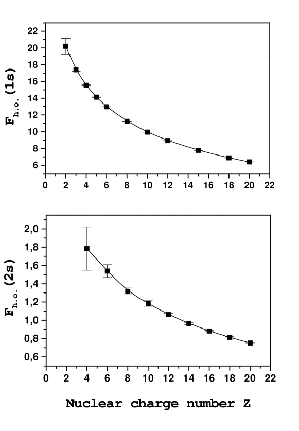
Figure 3: The higher-order self-energy contribution $F_{\rm h.o.}(Z\alpha)$ for the $1s$ and $2s$ electron $g$-factors in H-like ions.

The higher-order function $F_{\rm h.o.}(Z\alpha)$ for $1s$ and $2s$ states is plotted in Fig. 3.

VI Conclusion

In this paper we have presented our evaluation of the one-loop self-energy correction to the electron $g$-factor of $1s$ and $2s$ states in H-like ions. As compared to the previous calculations of this correction for the $1s$ state, an improvement of accuracy of about an order of magnitude has been achieved in the low-$Z$ region. For the most interesting experimental cases, H-like carbon and oxygen, our calculation improved the accuracy of the theoretical prediction for the $g$-factor by a factor of 3 for carbon and by a factor of 2 for oxygen Yerokhin02 , which reduced the uncertainty of the electron-mass determination based on these values. The new value for the electron mass is Haeffner00 ; Yerokhin02

$$m_{e}=0.000\,548\,579\,909\,29\,(29)(8)\,,$$ (104)

where the first uncertainty originates from the experimental value for the ratio of the electronic Larmor precession frequency and the cyclotron frequency of the ion in the trap, and the second error comes from the theoretical value for the bound-electron $g$-factor.

Appendix A Free one-loop functions

The free self-energy function in the Feynman gauge and in $D$ dimensions is given by

$$\Sigma^{(0)}(p)=-4\pi i\alpha\mu^{2\epsilon}\int\frac{d^{D}k}{(2\pi)^{D}}\frac{1}{k^{2}}\gamma_{\sigma}\frac{p\!\!\!/-k\!\!\!/+m}{(p-k)^{2}-m^{2}}\gamma^{\sigma}\,.$$ (105)

UV divergences in the above expression are regularized by working in $D=4-2\epsilon$ dimensions. The mass parameter $\mu$ is introduced in order to keep the proper dimension of the interaction term in the Lagrangian. We separate the UV-finite part of the self-energy function $\Sigma_{R}^{(0)}$ as follows

$$\Sigma^{(0)}(p)=\delta m-\frac{\alpha C_{\epsilon}}{4\pi\epsilon}(p\!\!\!/-m)+\Sigma^{(0)}_{R}(p)\,,$$ (106)

where the mass counterterm is given by

$$\delta m=\frac{\alpha C_{\epsilon}}{4\pi\epsilon}\,\frac{3-2\epsilon}{1-2\epsilon}\,m\,,$$ (107)

and

$$C_{\epsilon}=\Gamma(1+\epsilon)(4\pi)^{\epsilon}\left(\frac{\mu^{2}}{m^{2}}\right)^{\epsilon}\,.$$ (108)

In the limit $\epsilon\to 0$, the renormalized part of the self-energy function is given by

$$\Sigma^{(0)}_{R}(p) = \frac{\alpha}{4\pi}\Biggl{[}2m\left(1+\frac{2\rho}{1-\rho}\ln\rho\right)$$ (109)

$$-p\!\!\!/\,\frac{2-\rho}{1-\rho}\left(1+\frac{\rho}{1-\rho}\ln\rho\right)\Biggr{]}\,,$$

where $\rho=(m^{2}-p^{2})/m^{2}$.

The free vertex function in the Feynman gauge and in $D$ dimensions is written as

$$\Gamma^{\mu}(p,{p^{\prime}}) = -4\pi i\alpha\,\mu^{2\epsilon}\int\frac{d^{D}k}{(2\pi)^{D}}\frac{1}{k^{2}}\gamma_{\sigma}$$ (110)

$$\times\frac{p\!\!\!/-k\!\!\!/+m}{(p-k)^{2}-m^{2}}\gamma^{\mu}\frac{p\!\!\!/^{{}^{\prime}}-k\!\!\!/+m}{({p^{\prime}}-k)^{2}-m^{2}}\gamma^{\sigma}\,.$$

The divergent part of the vertex function can be separated in the form

$$\Gamma^{\mu}(p,p^{\prime})=\frac{\alpha C_{\epsilon}}{4\pi\epsilon}\gamma^{\mu}+\Gamma^{\mu}_{R}(p,p^{\prime})\,.$$ (111)

Here we present an explicit expression only for the time component of the renormalized vertex function $\Gamma^{\mu}_{R}$ omitting terms of order $\epsilon$ and higher and assuming that $p^{0}={p^{\prime}}^{0}=\varepsilon_{a}$,

$$\Gamma^{0}_{R}(p,p^{\prime}) = \frac{\alpha}{2\pi}\int_{0}^{1}dx\,dy\,\frac{1}{N}\Bigl{[}A\gamma_{0}$$ (112)

$$+\varepsilon_{a}Bp\!\!\!/+\varepsilon_{a}Cp\!\!\!/^{\prime}+Dp\!\!\!/\gamma_{0}p\!\!\!/^{\prime}+\varepsilon_{a}H\Bigr{]}\,,$$

where

$$A = a+m^{2}-N\left(\frac{3}{4}+x\ln N\right)\,,$$

$$B = 2(1-xy)(1-x)\,,$$

$$C = 2(1-x+xy)(1-x)\,,$$ (113)

$$D = -(1-x)\,,$$

$$H = -4m(1-x)\,,$$

and

$$a = xy(1-xy)p^{2}+x(1-y)(1-x+xy){p^{\prime}}^{2}$$ (114)

$$-2(1-xy)(1-x+xy)(p\cdot p^{\prime})\,,$$

$$N=x\left[yp+(1-y)p^{\prime}\right]^{2}+ym^{2}\rho+(1-y)m^{2}\rho^{\prime}\,.$$ (115)

The integration over one of the Feynman parameters in Eq. (112) can easily be carried out leading to an expression, equivalent to that in Yerokhin99 . However, we prefer to keep the vertex function in a more compact form (112) here.

For carrying out angular integrations, we introduce the scalar functions ${\cal F}_{1,2}$ that depend on $p_{r}=|{\bf p}|$, $p_{r}^{\prime}=|{\bf p}^{\prime}|$, and $\xi=\hat{{\bf p}}\cdot\hat{\bf p}^{\prime}$ only,

$$\displaystyle\overline{\psi}_{a}\,({\bf p})\Gamma^{0}_{R}(p,p^{\prime})\,\psi_{a}({\bf p}^{\prime})=\frac{\alpha}{2\pi}\int_{0}^{1}dx\,dy\,\frac{1}{N}$$

$$\displaystyle\times\biggl{[}{\cal F}_{1}\,\chi^{{\dagger}}_{+}(\hat{{\bf p}})\,\chi_{+}(\hat{\bf p}^{\prime})+{\cal F}_{2}\,\chi^{{\dagger}}_{-}(\hat{{\bf p}})\,\chi_{-}(\hat{\bf p}^{\prime})\biggr{]}\,,$$ (116)

$${\cal F}_{1} = (A+\varepsilon_{a}H)g_{a}g_{a}^{\prime}+\varepsilon_{a}B(\varepsilon_{a}g_{a}+p_{r}f_{a})g_{a}^{\prime}$$ (117)

$$+\varepsilon_{a}Cg_{a}(\varepsilon_{a}g_{a}^{\prime}+p_{r}^{\prime}f_{a}^{\prime})$$

$$+D(\varepsilon_{a}g_{a}+p_{r}f_{a})(\varepsilon_{a}g_{a}^{\prime}+p_{r}^{\prime}f_{a}^{\prime})\,,$$

$${\cal F}_{2} = (A-\varepsilon_{a}H)f_{a}f_{a}^{\prime}+\varepsilon_{a}B(\varepsilon_{a}f_{a}+p_{r}g_{a})f_{a}^{\prime}$$ (118)

$$+\varepsilon_{a}Cf_{a}(\varepsilon_{a}f_{a}^{\prime}+p_{r}^{\prime}g_{a}^{\prime})$$

$$+D(\varepsilon_{a}f_{a}+p_{r}g_{a})(\varepsilon_{a}f_{a}^{\prime}+p_{r}^{\prime}g_{a}^{\prime})\,,$$

where $\chi_{\pm}(\hat{{\bf p}})=\chi_{\pm\kappa_{a},m_{a}}(\hat{{\bf p}})$, and $g_{a}=g_{a}(p)$, $f_{a}=f_{a}(p)$, $g_{a}^{\prime}=g_{a}(p^{\prime})$, and $f_{a}^{\prime}=f_{a}(p^{\prime})$ are the radial components of the valence wave function.

Table 3: The one-loop self-energy correction to the $1s$-electron $g$-factor for H-like ions. All values are absolute contributions to the $g$-factor ($1/\alpha=137.035\,989\,5$) and presented in units of $10^{-6}$ (ppm). Individual contributions are listed for the point nuclear model. $\Delta g_{\rm NS}$ denotes the nuclear-size correction calculated for the shell model of the nuclear-charge distribution. The labels ”pnt.” and ”ext.” refer to the point-nucleus and the extended-nucleus result, respectively.

$Z$	$\Delta g_{\rm ir}$		$\Delta g_{\rm vr}^{(0)}$		$\Delta g_{\rm vr}^{(1)}$		$\Delta g_{\rm vr}^{(2+)}$		$\Delta g_{\rm SE}$ (pnt.)		$\Delta g_{\rm NS}$		$\Delta g_{\rm SE}$ (ext.)
1	1.	52928	2320.	77563	0.	50250	0.	03305	2322.	84046(10)	0.	00000	2322.	84046(10)
													2322.	8404(9)a
2	5.	20640	2316.	00970	1.	55757	0.	13053	2322.	90420(9)	0.	00000	2322.	90420(9)
													2322.	9040(9)a
3	10.	52313	2309.	28506	2.	91759	0.	28869	2323.	01447(9)	0.	00000	2323.	01447(9)
													2323.	0140(9)a
4	17.	21613	2300.	99753	4.	45945	0.	50260	2323.	17571(9)	0.	00000	2323.	17571(9)
													2323.	1751(9)a
5	25.	10744	2291.	41521	6.	10392	0.	76661	2323.	39318(9)	0.	00000	2323.	39318(9)
									2323.	42(5)b			2323.	3928(9)a
6	34.	06467	2280.	73799	7.	79535	1.	07460	2323.	67261(9)	0.	00000	2323.	67261(9)
													2323.	6724(9)a
8	54.	78171	2256.	69788	11.	16571	1.	79701	2324.	44230(9)	-0.	00001	2324.	44229(9)
													2324.	4421(10)a
10	78.	74380	2229.	82629	14.	34905	2.	61754	2325.	53668(10)	-0.	00002	2325.	53666(10)
									2325.	28b			2325.	5355(10)a
12	105.	51169	2200.	79830	17.	21623	3.	48376	2327.	00998(12)	-0.	00005	2327.	00993(12)
													2327.	0103(12)a
15	150.	23524	2154.	28732	20.	77184	4.	75746	2330.	05186(16)	-0.	00011	2330.	05175(16)
									2329.	79b			2330.	051(1)a
18	199.	76448	2105.	29703	23.	34254	5.	85654	2334.	26059(20)	-0.	00029	2334.	26030(20)
													2334.	262(2)a
20	235.	17645	2071.	71455	24.	49971	6.	41815	2337.	80885(24)	-0.	00052	2337.	80833(24)
									2337.	50b			2337.	86(1)a
24	311.	21758	2003.	24295	25.	53187	6.	95150	2346.	9439(3)	-0.	0015	2346.	9424(3)
													2346.	92(1)a
30	437.	19791	1899.	42146	24.	22809	5.	76765	2366.	6151(3)	-0.	0057	2366.	6094(3)
									2366.	77b			2366.	59(1)a
32	482.	18213	1864.	94188	23.	14976	4.	73024	2375.	0040(4)	-0.	0088	2374.	9952(4)
													2374.	97(1)a
40	676.	59132	1729.	56158	16.	47453	$-$3.	19027	2419.	4372(5)	-0.	0349	2419.	4023(5)
									2419.	45b			2419.	39(1)a
50	952.	87040	1569.	36938	5.	18971	$-$22.	43986	2504.	9896(7)	-0.	1615	2504.	8281(7)
									2504.	09b			2504.	827(8)a
54	1074.	52868	1508.	85111	0.	51786	$-$33.	12979	2550.	768(2)	-0.	282	2550.	486(2)
													2550.	487(8)a
60	1270.	36538	1422.	34049	$-$6.	00306	$-$52.	2051	2634.	498(3)	-0.	610	2633.	888(3)
									2634.	54b			2633.	895(9)a
70	1638.	25837	1290.	32234	$-$14.	07335	$-$90.	9411	2823.	566(5)	-2.	193	2821.	373(5)
									2823.	39b			2821.	39(1)a
80	2072.	57316	1174.	47096	$-$16.	61904	$-$135.	1054	3095.	320(10)	-6.	913	3088.	407(10)
									3095.	34b			3088.	46(2)a
82	2169.	55512	1153.	32686	$-$16.	29951	$-$144.	1073	3162.	475(12)	-8.	687	3153.	788(12)
													3153.	85(2)a
90	2601.	21377	1075.	78727	$-$11.	90297	$-$178.	5734	3486.	525(20)	-22.	32	3464.	205(20)
									3486.	56(3)a			3464.	35(2)a
									3487.	30b
92	2722.	17025	1058.	21204	$-$9.	99010	$-$186.	3945	3583.	998(20)	-28.	12	3555.	878(20)
													3556.	05(2)a

Table 3: $1s$ $g$-factor. (continued)

^a Ref. Beier00 , ^b Ref. Blundell97 .

Table 4: Various contributions to the one-loop self-energy correction to the $2s$-electron $g$-factor for H-like ions for the point nuclear model. All values are absolute contributions to the $g$-factor ($1/\alpha=137.035\,989\,5$) and presented in units of $10^{-6}$ (ppm).

$Z$	$\Delta g_{\rm ir}$		$\Delta g_{\rm vr}^{(0)}$		$\Delta g_{\rm vr}^{(1)}$		$\Delta g_{\rm vr}^{(2+)}$		$\Delta g_{\rm SE}$ (pnt.)
2	1.	4905	2320.	7711	0.	4471	0.	1317	2322.	8404(3)
4	5.	0539	2315.	9889	1.	3379	0.	5245	2322.	9051(4)
6	10.	1863	2309.	2305	2.	4286	1.	1729	2323.	0183(6)
8	16.	629	2300.	886	3.	600	2.	070	2323.	185(1)
10	24.	209	2291.	216	4.	778	3.	210	2323.	413(2)
12	32.	796	2280.	417	5.	909	4.	585	2323.	707(2)
14	42.	290	2268.	639	6.	956	6.	188	2324.	074(3)
16	52.	609	2256.	005	7.	892	8.	014	2324.	520(3)
18	63.	683	2242.	618	8.	696	10.	056	2325.	052(5)
20	75.	453	2228.	563	9.	351	12.	307	2325.	674(5)
24	100.	887	2198.	735	10.	177	17.	427	2327.	225(5)
30	143.	170	2150.	542	10.	109	26.	584	2330.	405(5)
32	158.	234	2133.	739	9.	728	30.	024	2331.	726(6)
40	222.	652	2063.	747	6.	429	45.	708	2338.	536(8)
50	311.	098	1971.	870	$-$1.	448	69.	823	2351.	343(9)
54	348.	579	1934.	243	$-$5.	641	81.	003	2358.	184(9)
60	406.	838	1877.	219	$-$12.	891	99.	640	2370.	807(9)
70	509.	241	1781.	353	$-$27.	042	136.	596	2400.	149(9)
80	619.	038	1685.	423	$-$42.	849	183.	153	2444.	765(9)
82	642.	093	1666.	316	$-$46.	101	193.	936	2456.	245(9)
83	653.	785	1656.	779	$-$47.	729	199.	543	2462.	378(9)
90	739.	302	1590.	411	$-$59.	021	243.	372	2514.	064(9)
92	765.	177	1571.	607	$-$62.	163	257.	585	2532.	207(9)

Table 4: $2s$ $g$-factor. (continued)

Figure 1: Feynman diagrams representing the self-energy correction to the bound-electron $g$-factor. The double line indicates the bound electron propagator and the wave line that ends with a cross denotes the interaction with the external magnetic field.

Figure 2: The potential expansion of the vertex diagram. The single line indicates the free-electron propagator and the dashed line denotes the interaction with the Coulomb field of the nucleus. The terms of the potential expansion are referred to as the zero-potential, one-potential, and many-potential contributions.

References

- (1) H. Häffner, T. Beier, N. Hermanspahn, H.-J. Kluge, W. Quint, S. Stahl, J. Verdú, and G. Werth, Phys. Rev. Lett. 85, 5308 (2000).
- (2) J.L. Verdú, T. Beier, S. Djekic, H. Häffner, H.-J. Kluge, W. Quint, T. Valenzuela, G. Werth, Can. J. Phys. 80, 1233 (2002).
- (3) P.J. Mohr and B.N. Taylor, Rev. Mod. Phys. 72, 351 (2000).
- (4) G. Werth, H. Häffner, N. Hermanspahn, H.-J. Kluge, W. Quint, J. Verdú, in The Hydrogen Atom, edited by S.G. Karshenboim et al. (Springer, Berlin, 2001), p. 204.
- (5) S.A. Blundell, K.T. Cheng, J. Sapirstein, Phys. Rev. A 55, 1857 (1997).
- (6) H. Persson, S. Salomonson, P. Sunnergren, and I. Lindgren, Phys. Rev. A 56, R2499 (1997).
- (7) T. Beier, I. Lindgren, H. Persson, S. Salomonson, P. Sunnergren, H. Häffner, and N. Hermanspahn, Phys. Rev. A 62, 032510 (2000).
- (8) A. Czarnecki, K. Melnikov, and A. Yelkhovsky, Phys. Rev. A 63, 012509 (2001).
- (9) S.G. Karshenboim, in The Hydrogen Atom, edited by S.G. Karshenboim et al. (Springer, Berlin, 2001), p. 651;
- (10) S. Karshenboim, V.G. Ivanov, and V.M. Shabaev, Can. J. Phys. 79, 81 (2001); Zh. Eksp. Teor. Fiz. 120, 546 (2001) [JETP 93, 477 (2001)].
- (11) V.M. Shabaev, Phys. Rev. A 64, 052104 (2001).
- (12) A.P. Martynenko and R.N. Faustov, Zh. Eksp. Teor. Fiz. 120, 539 (2001) [JETP 93, 471 (2001)].
- (13) D.A. Glazov, V.M. Shabaev, Phys. Lett. A 297, 408 (2002).
- (14) T. Beier, H. Häffner, N. Hermanspahn, S.G. Karshenboim, H.-J. Kluge, W. Quint, S. Stahl, J. Verdú, and G. Werth, Phys. Rev. Lett. 88, 011603 (2002).
- (15) V.M. Shabaev and V.A. Yerokhin, Phys. Rev. Lett. 88, 091801 (2002).
- (16) A.V. Nefiodov, G. Plunien, and G. Soff, Phys. Rev. Lett. 89, 081802 (2002).
- (17) V.A. Yerokhin, P. Indelicato, and V.M. Shabaev, Phys. Rev. Lett. 89, 143001 (2002).
- (18) V.M. Shabaev, D.A. Glazov, M.B. Shabaeva, V.A. Yerokhin, G. Plunien, and G. Soff, Phys. Rev. A 65, 062104 (2002).
- (19) Z.-C. Yan, J. Phys. B 35, 1885 (2002).
- (20) V.A. Yerokhin, P. Indelicato, and V.M. Shabaev, Can. J. Phys. 80, 1249 (2002).
- (21) V.M. Shabaev, D.A. Glazov, M.B. Shabaeva, I.I. Tupitsyn, V.A. Yerokhin, T. Beier, G. Plunien, and G. Soff, Nucl. Instr. Meth. Phys. Res. B 205, 20, 2003.
- (22) G. Breit, Nature (London) 122, 649 (1928).
- (23) V.M. Shabaev, Phys. Rep. 356, 119 (2002).
- (24) P. Indelicato and P. Mohr, Theor. Chim. Acta 80, 207 (1991).
- (25) H. Persson, S.M. Schneider, W. Greiner, G. Soff, and I. Lindgren, Phys. Rev. Lett. 76, 1433 (1996).
- (26) V.M. Shabaev, J. Phys. B 24, 4479 (1991).
- (27) E.M. Rose, Relativistic Electron Theory (Whiley, New York, 1961).
- (28) D.A. Varshalovich, A.N. Moskalev, V.K. Khersonskii, Quantum Theory of Angular Momentum (World Scientific, Singapore, 1988).
- (29) V.A. Yerokhin and V. M. Shabaev, Phys. Rev. A 60, 800 (1999).
- (30) W.R. Johnson, S.A. Blundell and J. Sapirstein, Phys. Rev. A 37, 2764 (1988).
- (31) N.J. Snyderman, Ann. Phys. (N.Y.) 211, 43 (1991).
- (32) P. Indelicato, P.J. Mohr, Phys. Rev. A 46, 172-185 (1992).
- (33) P. Indelicato, P.J. Mohr, Phys. Rev. A 58, 165-189 (1998).
- (34) P. Indelicato, P.J. Mohr, Phys. Rev. A 63, 052507 (2001).
- (35) P.J. Mohr, Ann. Phys. (N.Y.) 88, 26 (1974).
- (36) V.A. Yerokhin and V.M. Shabaev, Phys. Rev. A 64, 012506 (2001).
- (37) H. Grotch, Phys. Rev. Lett. 24, 39 (1970).