From molecular dynamics to coarse self-similar solutions:
A simple example using equation-free computation.

Abstract

In the context of the recently developed “equation-free” approach to the computer-assisted analysis of complex systems, we illustrate the computation of coarsely self-similar solutions. Dynamic renormalization and fixed point algorithms for the macroscopic density dynamics are applied to the results of short bursts of appropriately initialized molecular dynamics in a simple diffusion simulation. The approach holds promise for locating coarse self-similar solutions and the corresponding exponents in a variety of multiscale computational contexts.

Keywords: dynamic renormalization, equation-free, microscopic model, distribution function

1. Introduction

In contemporary scientific and engineering modeling we are often faced with situations where the best system models are available at a fine scale (e.g. atomistic, individual-based); yet we want to predict the behavior of the system at a much more coarse-grained, macroscopic level. In traditional modeling successful closures often allow us to write models directly at the coarse-grained, macroscopic level at which we want to model the behavior; typical examples include chemical kinetics closures in terms of reactant concentrations for reactor modeling, or Newton’s law of viscosity in the Navier-Stokes equations. Often, however, such accurate closures are not available, and the immense range of active scales (in space as well as time) precludes the practical prediction of macroscopic behavior through direct atomistic simulation.

The recently developed “equation free” approach to coarse-grained computer-assisted analysis of complex systems attempts to bridge this enormous scale gap when macroscopic equations conceptually exist, but are not available in closed form [1, 2, 3, 4, 5, 6, 7, 8]. The approach constitutes a bridge between traditional continuum numerical analysis and microscopic simulation. The main idea is to consider the microscopic simulation as a computational experiment which can be initialized and run at will. If a coarse-grained, macroscopic equation were available, traditional numerical tasks would involve repeated evaluations of the equation, and of its functional or parametric derivatives, at various values of the macroscopic state. The idea is to substitute these function evaluations with short bursts of appropriately initialized microscopic computational experimentation, from the results of which the requisite numerical quantities are estimated. The quasi-continuum method of Phillips, Ortiz and coworkers [9], as well as the optimal predictor approach of Chorin and coworkers [10] embody many of these features; see [7] for a discussion. The approach can be successfully combined with matrix-free iterative linear algebra to allow us to solve linear and nonlinear macroscopic equations, perform “coarse projective integration” as well as additional tasks like controller design and optimization without ever writing down the macroscopic equations in closed form. This is a system identification based, “closure on demand” approach.

Over the last few years we have demonstrated how to use this approach for the accelerated simulation and bifurcation analysis of the coarse-grained, expected behavior of kinetic Monte Carlo, Brownian Dynamics, Molecular Dynamics and Lattice-Boltzmann microscopic simulation codes, [1, 2, 3, 4, 5, 6, 7, 8, 11] as well as the solution of effective medium equations [12, 13] for media with spatially varying properties. The approach gives rise to two-level (conceptually possibly multi-level) codes. The “inner code” is the best microscopic simulation of the phenomenon at our disposal. The outer code, the “wrapper”, is typically templated on traditional continuum numerical analysis, and constitutes a protocol for the design of microscopic simulations and for processing their results towards a macroscopic modeling goal. Accelerated simulation, the location of coarse fixed points and their continuation and bifurcation analysis are typical such goals.

In many cases of interest, the macroscopic dynamics we explore do not involve stationary solutions, but rather traveling or self-similar solutions. In this paper we will show how to use the basic coarse timestepper methodology to construct dynamic renormalization algorithms for the location of coarse self-similar solutions and the corresponding similarity exponents by acting on a microscopic code directly. Our illustrative example – molecular diffusion in a thin two dimensional domain – is extremely simple, yet it does illustrate the basic ingredients of the approach.

The paper is organized as follows: In the next Section we will briefly describe template-based dynamic renormalization when macroscopic equations are explicitly available. In Section 3 we summarize the main components of the coarse timestepper, and, in particular, its modification for computation of self-similar solutions as fixed points of the appropriate discrete time map. Section 4 presents our illustrative examples for both coarse dynamic and coarse fixed point computations in a dynamic renormalization context. We conclude with a brief summary and outline of the scope of the method and some of the challenges we expect to arise in its wider application.

2. Dynamic renormalization in a continuum context

In problems with translational invariance, one often encounters traveling wave solutions – constant shape waves that move in space at constant speed. It is convenient (mathematically, computationally and practically) to study these solutions, and the transient approach to them, in a co-traveling frame. In this frame the traveling solution appears stationary, and it is much easier to study the transient approach to it and its stability unencumbered by its constant motion. Good techniques exist for computationally locating the translationally invariant solution along with its traveling speed as a nonlinear eigenvalue problem. During transient simulation, however, the solutions both travel and approach their ultimate, translationally invariant shape; the right speed for “moving along” with such a transient solution may change from moment to moment, and the best way to choose it is not transparent. In a recent paper Rowley and Marsden [14] described a template based approach that allows one to systematically recover such an appropriate instantaneous speed; as the transient solution asymptotically approaches the ultimate, translationally invariant, traveling wave, the speed from the template-based algorithm asymptotically approaches the correct traveling speed.

In a sequence of papers [15, 16, 17] we have shown how to adapt this approach from the computation of translationally invariant solutions to the case of scale invariant solutions – that is, solutions of dynamic equations that evolve across scales. Self-similar solutions [18, 19] are an important such class of scale-invariant solutions; in the same sense that it is practical to observe a traveling solution in a co-traveling frame, self-similar solutions are convenient to observe in a co-exploding or co-collapsing frame. Consider the rather general form of partial differential equation

$$u_{t}=D_{x}(u)$$ (1)

where the operator $D$ satisfies the scaling relation

$$D_{x}(Bf(x/A))=A^{a}B^{b}D_{y}(f(y)),{\rm~{}~{}~{}where~{}}y=x/A$$ (2)

for $A>0,B>0$, and $a$ and $b$ are constants. We assume that there exists a family of self-similar solutions,

$$u(x,t)=s^{\beta}U\left(\frac{x}{s^{\alpha}}\right);$$ (3)

where $s=|t-t^{*}|$ (for the case of finite time blow-up at $t=t^{*}$) or $s=t$ otherwise, and $U$ satisfies the ODE,

$$\sigma\beta U-\alpha yU_{y}=D_{y}(U),$$ (4)

where $y=x/(s^{\alpha})$ with $\sigma=sgn(t-t^{*})$ and

$$\beta-1=a\alpha+b\beta.$$ (5)

We are interested in locating the self-similar shape of the solution as well as both similarity exponents $\alpha$ and $\beta$: one more equation is needed for this latter task. Starting with the general scaling

$$u(x,t)=B(s)w(\frac{x}{A(s)},\tau(s))$$ (6)

where $A$, $B$ and $\tau$ are unknown functions, and setting $\tau_{s}(s)=\sigma A^{a}B^{b-1}$, the PDE becomes

$$w_{\tau}+\frac{B_{\tau}}{B}w-\frac{A_{\tau}}{A}yw_{y}=D_{y}(w),{\rm~{}~{}~{}where~{}}y=x/A(\tau).$$ (7)

This is the “co-exploding” or “co-collapsing” equation which, for self-similar problems, is analogous to the “co-traveling” equation for translationally invariant ones. Two additional constraints, frequently called pinning conditions, are needed to find both $A(\tau)$ and $B(\tau)$. There is some latitude in the selection of these conditions – different conditions correspond to different ways of “moving along with the solution across scales” before Eq. (7) reaches steady state, although all appropriate pinnings give the same self-similar shape and exponents [20]. In the spirit of Rowley and Marsden, we proposed in [15] that such conditions can be constructed by imposing relationships between the solution and (essentially arbitrary) template functions.

Since there are two degrees of freedom (“amplitude” and “width”) we must impose two pinning conditions. Once these have been imposed, we can use Eq. (7) to solve for $A(\tau)$ and $B(\tau)$: it is actually possible to eliminate the $A_{\tau}/A$ and $B_{\tau}/B$ terms in Eq. (7) to end up with a “co-exploding” PDE that we called in [15] MN-dynamics. When (and if) the solution of this PDE approaches an asymptotic steady state, we can compare coefficients in Eqs. (4) and (7) to find:

$$\frac{\alpha}{\beta}=\frac{\lim_{\tau\rightarrow\infty}A_{\tau}/A}{\lim_{\tau\rightarrow\infty}B_{\tau}/B}$$ (8)

Eqs. (5) and (8) allow us to obtain the scaling exponents $\alpha$ and $\beta$. A more detailed discussion can be found in [20]; the approach can be used to locate both types of self-similar solutions [18], and indeed in [15] it was used to locate both the Barenblatt and the Graveleau solutions of the porous medium equation.

In view of our illustrative example using molecular dynamics below, we briefly study the very simple case of the 1-dimensional diffusion equation,

$$u_{t}=u_{xx}.$$ (9)

The operator in this case is $D_{x}(u)=u_{xx}$. From Eq. (2), $b=1$ and $a=-2$. Eq. (5) then yields $\alpha=1/2$. For self-similar solutions of the second kind, $\alpha$ and $\beta$ cannot be computed a priori, and will be found as part of the solution process. For the two pinning conditions, we choose here to let $w$ satisfy the following relations to two given template functions, $T_{1}(y)$ and $T_{2}(y)$ respectively,

$$\int_{-\infty}^{+\infty}w(y,\tau)T_{1}(y)dy = 0$$ (10)

$$\int_{-\infty}^{+\infty}w(y,\tau)T_{2}(y)dy = 1.$$ (11)

These can be thought of as controlling the “width” and the amplitude of the solution. By multiplying Eq. (7) with each $T(y)$, integrating and using the above two equations, we can eliminate $A$ and $B$. A discussion of important technical conditions, having to do with the existence of these integrals over infinite domains, and the appropriate solution spaces, can be found in [34, 35]. (An alternative approach is to require that the difference between the solution of Eq. (7) and a template is minimized, as discussed in [15, 17].)

For our simple diffusion example, we set $T_{1}(y)$ to be

$$T_{1}(y)=\left\{\begin{array}[]{cc}1&{\rm for~{}}|y|\leq 1/2\\ -1&{\rm for~{}}|y|>1/2.\end{array}\right.$$ (12)

From Eqs. (7), (10), and (12) we get an equation for $A_{\tau}/A$. Since the subspace of solutions symmetric around $x=0$ is invariant, restricting our search to symmetric solutions we find that

$$\frac{A_{\tau}}{A}=-\frac{2w_{y}(0.5,\tau)}{w(0.5,\tau)}.$$ (13)

Similarly, if we set $T_{2}(y)=\delta(y)$ we get

$$\frac{B_{\tau}}{B}=w_{yy}(0,\tau).$$ (14)

Substituting these in Eq. (7) we get

$$w_{\tau}+w_{yy}(0,\tau)w+\frac{2w_{y}(0.5,\tau)}{w(0.5,\tau)}yw_{y}=w_{yy}.$$ (15)

For an initial condition consistent with the constraints and the symmetry we take

$$w(y,0)=\left\{\begin{array}[]{cc}1&{\rm for~{}}|y|\leq 1\\ 0&{\rm for~{}}|y|>1.\end{array}\right.$$ (16)

so that both Eqs. (10) and (11) are satisfied. Finally, we numerically integrate Eq. (15) to steady state, i.e. $\tau\rightarrow\infty$, and evaluate the exponent, $\beta$ from

$$\beta=-\frac{\alpha w(0.5,+\infty)w_{yy}(0,+\infty)}{2w_{y}(0.5,+\infty)}.$$ (17)

Another choice for $T_{2}(y)$ would be $T_{2}(y)=1$. Physically it corresponds to conservation of mass, and the same procedure leads to

$$w_{\tau}+\frac{2w_{y}(0.5,\tau)}{w(0.5,\tau)}(w+yw_{y})=w_{yy}.$$ (18)

Without any further integration, it is clear that $\beta=-\alpha=-1/2$.

The above methodology evolves the differential equation in a dynamically rescaled time and space frame. Figure 1a shows the solution of the diffusion equation (in the central portion of a large domain) for the initial condition above; as time progresses we know that the solution decays, but it also asymptotically approaches a (self-similarly decaying) Gaussian. (For clarity, the solution is shown over several small blocks of time, alhough the equation was also integrated over the “spaces” in the figure.) Figure 1b shows the same evolution in a rescaled frame using Eq. (15); the decay has now been removed through the template-based rescaling, and one only sees the transient approach to the self-similar shape (the Gaussian) consistent with the template-based pinning conditions. Figure 1c shows the same results in terms of cumulative material density and not the density itself; as we will discuss below, it is numerically more convenient in particle based simulation codes to work with the cumulative distribution function rather than the particle distribution function itself. It is interesting to consider the case in which we have a so-called “legacy code” – a code that evolves the original equation and which we can run but cannot modify. The so-called numerical analysis of legacy codes allows us to transform a direct legacy dynamic simulator, by “‘wrapping” a computational superstructure around it, into a code capable of performing a different set of tasks, for which the legacy simulator was not designed. In the dynamic renormalization case, we will compute self-similar solutions by evolving in physical variables and rescaling the results, as opposed to first obtaining and then evolving the rescaled equation. Our approach is a discrete-time approach (see also [12, 21]); pioneering work on dynamic renormalization, especially in the context of the Nonlinear Schrödinger Equation can be found in [22, 23, 24, 25, 26, 27, 28, 29, 30, 31].

3. Timestepping for coarse dynamic renormalization

As we discussed above, one can use a direct simulator of the original equation to converge computationally to a (stable) self-similar solution as follows. Starting with an initial profile, one evolves forward for a finite time; one then uses the template conditions to rescale the space variable for the final profile. The rescaled profile is then given as an initial condition to the original equation, which is again evolved over finite time; the space variable is rescaled, and the procedure is iterated until the shape converges to a member of the family of self-similar shapes. The idea here is that rescaling, and then evolving the rescaled equation for a finite time, commutes with evolving in physical space and then rescaling the result (see Figure 2). Also, while stable self-similar solutions can be found by such dynamic rescaling and forward integration, they can also be found – and so can unstable self-similar solutions – through fixed point algorithms (like Newton-Raphson). Indeed, if we call $\Phi_{T}(w(y))$ the result of integrating the rescaled equation with initial condition $w(y)$ over time $T$, the self-similar solution satisfies

$$w(y)-\Phi_{T}(w(y))=0.$$ (19)

We have shown in the past how matrix-free iterative linear algebra techniques [32] can be used to converge to solutions of such problems even when the only available tool is a subroutine that numerically computes $\Phi_{T}(w(y))$. The original inspiration for this work was the so-called Recursive Projection Method (RPM) of Shroff and Keller [33], who used this subroutine (the timestepper) and a computational superstructure (the RPM wrapper) to construct a fixed point algorithm. Under appropriate conditions this algorithm accelerates the computation of stable fixed points and also stabilizes the computation of dynamically unstable ones. In effect, timestepping combined with matrix-free techniques “fools” a dynamic simulator into becoming a fixed point solver. It is important to note in this entire exposition that we have essentially ignored here the role of the boundary conditions for the original and the rescaled equation, assuming we are solving in sufficiently large domains and for sufficiently short times; it is conceivable that weighted Sobolev spaces must be used in order to avoid spurious numerical oscillations [35]. This is an important issue which must be studied carefully; yet, as we will see, for our simple problem this does not create major computational difficulties.

We now return to the premise of our introduction: we have a microscopic code (e.g. molecular dynamics, evolving a distribution of molecules); yet we believe that the coarse-grained, macroscopic behavior of the statistics of the simulation satisfies a macroscopic equation that possesses self-similar solutions. We will find these solutions through what we will call the “coarse timestepper”, which we have extensively discussed in [1, 2, 3, 4, 5, 6, 7, 8, 11], and which – for the case of dynamic renormalization – is illustrated in Figure 3. This “coarse dynamically renormalized timestepper” consists of the following elements:

1. Choose the statistics of interest for describing the coarse-grained behavior of the system and an appropriate representation for them. In this case the concentration profile in one space dimension is the appropriate macroscopic observable; it is the zeroth moment of the distribution of molecules over velocities (and over the second, “thin” dimension). It is more convenient to use the particle instantaneous Cumulative Distribution Function; assuming it is smooth enough, one can use a low-dimensional description of it based on the first few of an appropriate sequence of orthogonal polynomials [36, 37]. We will call this the macroscopic description, ${\bf u}$. These choices determine a restriction operator, ${\cal M}$, from the microscopic-level description, ${\bf U}$ (particle coordinates) to the macroscopic description: ${\bf u}={\cal M}{\bf U}$.

2. Choose an appropriate lifting operator, ${\cal\mu}$, from the macroscopic description, ${\bf u}$, to the microscopic description, ${\bf U}$. In our case we make random particle assignments consistent with the macroscopic CDF. ${\cal\mu}$ should have the property that ${\cal M}{\cal\mu}$ is the identity (${\cal M}{\cal\mu}=I$). In other words, lifting from the macroscopic to the microscopic and then restricting (projecting) down again should have no effect (except round-off).

3. From an initial value at the microscopic level, ${\bf U}(t_{0})$, run the microscopic simulator (the fine timestepper) for a (relatively short) macroscopic reporting horizon $T$ generating the values ${\bf U}(T)$. We may have to repeat this for several microscopic initial conditions ${\bf U}_{i}(t_{0})$, consistent with the same macroscopic one ${\bf u}(t_{0})$, for variance reduction purposes.

4. Obtain the restriction ${\bf u}(T)={\cal M}{\bf U}(T)$ (the average restriction, in the case of many copies).

5. Rescale ${\bf u}(T)$ to obtain ${\bf u_{R}(T)}$ (using the template conditions).

6. Lift ${\bf u_{R}}(T)$ to get a new consistent microscopic ${\bf U}={\cal\mu}{\bf u_{R}}(T)$ and use it as a new starting value for repeating steps 3 to 6.

Since the diffusion equation has a stable self-similar solution, one can simply repeat the above procedure and observe the approach of the statistics of the molecular description to the Gaussian; the repeated dynamic coarse rescaling helps avoid the continuous decay of the direct simulation towards zero. Alternatively, as we will show, one can use coarse fixed point algorithms (such as Newton-Raphson) to converge iteratively to the fixed point of the coarse rescaled timestepper (as opposed to repeatedly integrating and rescaling). Finally, while this is a problem where the exponents are known a priori through scaling, the formulas presented in Section 2 and the rescaling history upon convergence to the self-similar solution helps us estimate the limiting values of $A_{\tau}/A$ and $B_{\tau}/B$. This will then help recover, through Eqs. (5) and (8) the self-similarity exponents for type-2 self-similar solutions.

4. The computational experiment

In this Section we outline the data collection procedure from the molecular dynamics simulation. A standard Lennard-Jones potential was used, i.e.

$$V(r)=4\epsilon[(\sigma/r)^{12}-(\sigma/r)^{6}]$$ (20)

with cutoff distance $2.5\sigma$. In what follows all results will be given in reduced units, i.e., length in units of $\sigma$, time in units of $(m\sigma^{2}/\epsilon)^{1/2}$. The simulation was performed in a quasi-1d box with size $400\times 10$, and periodic boundary conditions in both $x$ and $y$ directions. We use $T=1.0$, $\rho=0.5$. The domain for such a simulation time was “large enough” to appear infinite over the time of our simulation.

First, the system is allowed to evolve to thermal equilibrium (as evidenced by stationarity of the average kinetic energy of the particles). After some simulation time we record our first equilibrium configuration, and “reset the clock” to $t=0$. Subsequent equilibrium configurations are recorded at later times. To model the diffusion process, a fraction of the particles were colored according to prescribed distributions (consistent with given density profiles), and their positions in the later configurations were tracked.

We are going to work with a single-variable cumulative distribution function (CDF) [36]. Suppose that $N$ particles are colored, and the $i$-th particle is in position $x_{i}$. Given all the colored particle positions, we can immediately obtain their empirical CDF by sorting them, that is, relabeling them so that $x_{i}\geq x_{i-1},~{}0<i\leq N$, and plotting $x_{i}$ vs $p_{i}=(i-0.5)/N)$. We use the CDF rather than the density function because it is trivial to generate the empirical CDF while it is computationally difficult and error-prone to compute the empirical density function which is the (ill-defined) derivative of the CDF.

Using only the $x$ coordinate of particle positions is justified by our quasi-1d simulation box. In fact, it is easier to work with the inverse CDF, or ICDF, $Q(p)$. It gives the the $x$ coordinate of a given particle position, $i$, and it can be read off directly as $Q(p(i))$. Such continuous ICDFs can then be microscopically approximated by coloring the particle with the nearest $x$-coordinate value in the simulation box. Using the data (positions of colored particles) from later time configurations, we can estimate the dynamics of the CDF (or ICDF) evolution.

In the first numerical experiments, we ran the systems for short bursts of time, then applied templates to rescale the ICDF. Because the number of colored particles we used is constant, mass is automatically conserved, so that only one additional template, $T_{1}$, is needed for dynamic rescaling. For this second template, we computed the slope of the center 20% of the colored particles by linear least squares, and normalized it to a fixed value. This implied a simple rescaling of the $x$ coordinates of the computed colored particle positions. These rescaled $x$ values were then used to “lift” the rescaled ICDF: we selected the closest particles to these coordinates in the full set, and colored them for a further short burst of computation. Using this “evolve–restrict–rescale–lift” procedure repeatedly, the correct functional form of the self-similar solution will arise asymptotically: the shape of the coarse-grained description (the ICDF) converges to the inverse of the integral of a Gaussian (see Figure 4.)

In the second numerical experiment, we used a Newton iteration to converge to the stationary, dynamically renormalized solution – that is, the self-similar solution. To do this, we need to restrict the CDF to a finite (preferably low-dimensional) approximate representation. Orthogonal polynomials usually provide computationally simple approximations, but unfortunately they are not useful for the CDF which has a possible support from $-\infty$ to $+\infty$ (that is, the CDF is $c(x)$ where $x$ has a potentially infinite range; $c(x)$ must be monotone non-decreasing and must lie between $0$ and $1$). This is a second, and more important, reason for using the ICDF, $x(p)$ where $p$ lies in $[0,1]$. This function can easily be approximated by a low-degree polynomial over its range.

We wish to find a polynomial approximation, $Q(p)$, that approximates the computed positions. That is, on the finite set of points, $\{x_{i}\}$, corresponding to $\{p_{i}\}=\{(i-0.5)/N\}$, we would like $Q(p_{i})\approx x_{i}$. This provides us our restriction of the microscopic data. Then we can evaluate $Q$ at any point in [0,1] in the lifting process. (Typically, we will evaluate it at each $p_{i}$ to get an approximate $x_{i}$.) We are interested in minimizing the error of the approximation only at the arguments $p_{i},i=1,\cdots,N$. If we use least squares approximation with weights $w_{i}$ we thus want to minimize

$$\sum_{i=1}^{N}[x_{i}-Q(p_{i})]^{2}w_{i}.$$ (21)

In the experiments we used unit weights, $w_{i}=1$. The best way to do this computationally is to create a basis for the $N$-dimensional vector space, $\phi_{s},s=1,\cdots,N$ such that the $s$-th basis vector, $\phi_{s}$ has its $i$-th element defined as the value of an $(s-1)$-st degree polynomial evaluated at $p_{i}$, that is, $\phi_{si}=q_{s}(p_{i}).$ To make this basis set orthonormal, we require that

$$\langle\phi_{s},\phi_{t}\rangle\equiv\sum_{i=1}^{N}q_{s}(p_{i})q_{t}(p_{i})=\delta_{st}.$$ (22)

The $q$ polynomials thus defined are scalar multiples of the orthogonal polynomials defined in the usual way from the L2 norm over the unit interval.

Since the steady state solution of $w$ is symmetric, its ICDF will be an odd function of $p-0.5$. For this reason, we chose orthogonal polynomials on the finite set $\{-0.5+(i-0.5)/N\}$. For the purposes of the Newton iteration we considered a fifth degree polynomial representation of the ICDF written as

$$Q(p)=c_{1}\phi_{1}(p-0.5)+c_{3}\phi_{3}(p-0.5)+c_{5}\phi_{5}(p-0.5).$$ (23)

The constancy of the number of colored particles provides one template condition for rescaling. In this example, the second template condition was applied by requiring that $c_{1}$ be constant. After each burst of microscopic simulation, the restriction to form Eq. (23) was performed, and then the polynomial was divided by $c_{1}$ to get a scaled polynomial with $c_{1}=1$. The use of a small number of features of the solution (“observables”) for the Newton iteration with timesteppers is justified when the long-term dynamics of an evolution equation are low-dimensional (i.e. lie on an attracting low-dimensional manifold parameterized by a small number of “modes” or “observables”, like the $c_{i}$ here).

We can perform variance reduction by using multiple copies. In this case, because the box is large enough and the problem is translationally invariant, different parts of the box can be used for different realizations of evolving CDFs (and each can be colored differently so that they can be distinguished, as long as they are far enough apart to be uncorrelated). We take an average of several such realizations (typically 10, or, for stationary point computations, 100).

5. Results and discussion

In order to demonstrate how rescaling can accelerate convergence to the self-similar shape we design a piecewise linear CDF with fewer particles in the tail part, as shown in Fig. 4. We evolve until $t=300$ and rescale, but the tail part of the rescaled CDF is still significantly away from the Gaussian. In the right lower corner of Figure 4 snapshots of the colored particles in the simulation box at $t=300$ and after rescaling and lifting are shown. It takes five repetitions of the procedure (evolving and rescaling) until the rescaled CDF converges visibly to the Gaussian curve.

To reduce the effect of noise in estimating functional derivatives or the fixed point algorithm, $200$ copies of the system at equilibrium are let to run further until $t=1000$. A perturbation as large as $3\%$ of the initial values of the coarse variables (the $c_{i}$) is necessary to ensure a meaningful finite difference estimate of the $2\times 2$ Jacobian of the coarse self-similar fixed point computation. As shown in Table 1, the fixed point values of $c_{3}$, $c_{5}$ are $c_{3}/c_{1}\approx 0.18$, $c_{5}/c_{1}\approx 0.075$, respectively.

Comparing the fixed point solution shape (reconstructed based only on the computed polynomial terms) with the Gaussian, the only visual difference is at the tail part, where very few particles exist. The actual solution we have found (the result of initializing symmetrically with given values for the first three odd $c_{i}$ and zero for the remaining $c_{i}$, evolving for the given time horizon, and rescaling so that the first three odd $c_{i}$ have the same values) has now acquired components in the remaining odd $c_{i}$, and is closer to the Gaussian than its truncation. Using molecular dynamics constrained on these three macroscopic observables will give us a better estimate of the macroscopic fixed point we located (see [38] for further discussion). Different basis sets for the approximation can be used if significant information in the tails is not well captured this way.

The process we have described allows us to compute the shape of the self similar solution. If we also need the exponents $\alpha$ and $\beta$ in Eq. (3) we have to know $a$ and $b$ defined in Eq. (2) and the value of $(\lim A_{\tau}/A)/(\lim B_{\tau}/B)$ so that we can apply Eqs. (5) and (8). When an equation is known, $a$ and $b$ are obtained by inspection. When it is not known in closed form, ideas similar to those used in [5] can be used to test the existence of self-similarity and estimate $a$ and $b$; in particular, this will involve the microscopic simulation for short periods to estimate $du/dt$ in Eq. (1) from multiple initial conditions that are scaled (in amplitude and space) versions of each other.

Once a coarse self-similar solution has been converged to, whether through integration or Newton-Raphson of the appropriately renormalized coarse dynamics, we can use again short simulations to estimate $A_{t}/A$ and $B_{t}/B$. Starting a microscopic simulation at time $t$ and evolving for time $d$, the relative values of $A$ and $B$, that is, $A(t+d)/A(t)$ and $B(t+d)/B(t)$, can be obtained from the scaling needed to re-impose the template conditions. These lead to approximations of $A_{t}/A$ and $B_{t}/B$, from which $\alpha/\beta$ can be estimated using Eq. (8).

6. Conclusions

We have described a systematic approach for the computation of coarse self-similar solutions in situations where the only available model is a microscopic (in this case molecular dynamics) simulator. The procedure uses short, appropriately initialized bursts of MD simulation to estimate the coarse timestepper of the template-based renormalization flow for the process. In the case we studied here, a $2\times 2$ numerical Jacobian for the Newton iteration was sufficient; more generally, matrix-free techniques can be combined with this coarse renormalized timestepper to compute stable as well as unstable self-similar solutions, compute “finite times to blow-up” in the appropriate cases as well as estimate the self-similarity exponents. The stability of the self-similar solutions in the co-exploding frame can be probed through the same coarse renormalized timestepper and matrix-free eigenanalysis techniques. It is also possible to combine the equation-free algorithms presented here with the so-called ”gaptooth scheme” and ”patch dynamics” [6, 39, 40, 7]. The microscopic computations are not performed across all of space, but only in relatively small physical domains (”teeth” separated by gaps and connected through appropriate boundary conditions). This approach exploits smoothness of the macroscopic observables (e.g. particle density) in space as well as time, in order to further reduce the microscopic simulation necessary to compute coarse self-similar solutions.

It is important to notice that the results are valid over some scaling regime, while for model equations they in principle hold over all scales. In the context of non-Newtonian fluid mechanics, such techniques could assist the quantitative detection of self-similarity in phenomena such as spreading [41, 42]. More ambitiously, one may envision the use of equation-free coarse renormalization to study the self-similar behavior of the evolution of spectra in turbulence studies [43].

Extensive research explores the onset of dynamic self-similarity as operating parameters vary [16] as well as the study of asymptotically self-similar solutions. Self-similar solutions may explode or collapse in infinite time (as in the case of the diffusion equation we studied here) or can have finite-time blow-ups, in which the solution increasingly accelerates in time. Conversely it is possible to have self-similar solutions which progressively decelerate in time; this may be relevant in the description of glassy dynamics [44], and it is conceivable that extensions of the approach presented here may assist in accelerating the computation of self-similar solutions that progressively slow down.

Figure Captions

Fig. 1 a) Time evolution of an initial rectangular density profile by the 1d diffusion equation, Eq. (9). b) Dynamically renormalized evolution of the same shape using Eq. (15). c) Cumulative distribution function representation of (b).

Fig. 2 Rescaling the finite time direct simulation commutes with the dynamic renormalization flow.

Fig. 3 Schematic view of the coarse dynamically renormalized timestepper.

Fig. 4 Coarse evolution of the cumulative distribution function using coarse renormalized timestepping, starting with a piecewise linear CDF. The inset shows (top) a snapshot obtained around the center of the computational domain after $t=300$, as well as (bottom) the result of restricting, rescaling and lifting this snapshot.

Table 1: Dynamically renormalized fixed point computation using Newton-Raphson.

iteration	$c_{3}/c_{1}$	$c_{5}/c_{1}$	$|\Delta c_{3}/c_{1}|+|\Delta c_{5}/c_{1}|$
0	0	1	1.09626
1	0.278266	0.156855	0.138427
2	0.188089	0.0816683	0.01203
3	0.176717	0.0745533	0.00207797
4	0.178675	0.0747852	0.000377391

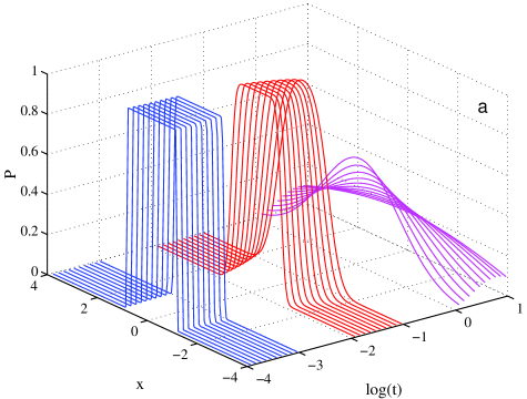
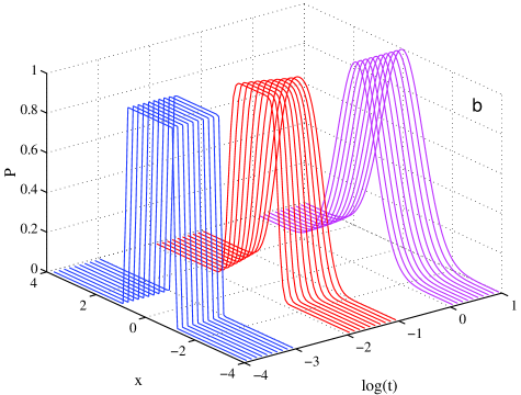
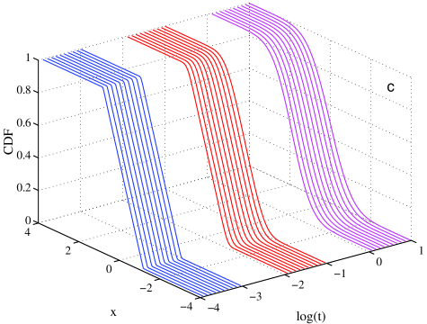
Figure 1: a) Time evolution of an initial rectangular density profile by the 1d diffusion equation, Eq. (9). b) Dynamically renormalized evolution of the same shape using Eq. (15). c) Cumulative distribution function representation of (b).

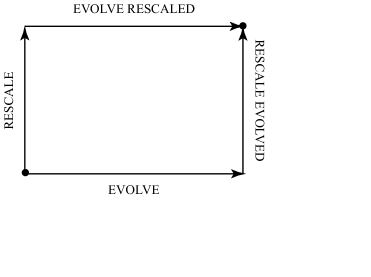
Figure 2: Rescaling the finite time direct simulation commutes with the dynamic renormalization flow.

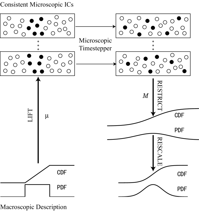
Figure 3: Schematic view of the coarse dynamically renormalized timestepper.

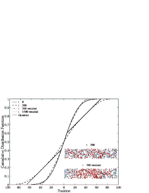
Figure 4: Coarse evolution of the cumulative distribution function using coarse renormalized timestepping, starting with a piecewise linear CDF. The inset shows (top) a snapshot obtained around the center of the computational domain after $t=300$, as well as (bottom) the result of restricting, rescaling and lifting this snapshot.

References

- [1] K. Theodoropoulos, Y. H. Qian, and I. G. Kevrekidis, Coarse stability and bifurcation analysis using timesteppers: a reaction diffusion example, Proc. Natl. Acad. Sci. USA, 97 (2000) 9840–9843.
- [2] C. W. Gear, I. G. Kevrekidis, and C. Theodoropoulos, Coarse integration/bifurcation analysis via microscopic simulations: micro-Galerkin methods, Comp. Chem. Eng., 26 (2002) 941–963.
- [3] A. G. Makeev, D. Maroudas, A. Z. Panagiotopoulos, and I. G. Kevrekidis, Coarse bifurcation analysis of kinetic Monte Carlo simulations: a lattice gas model with lateral interactions, J. Chem. Phys., 117 (2002) 8229–8240.
- [4] C. Siettos, M. D. Graham, and I. G. Kevrekidis, Coarse Brownian dynamics for nematic liquid crystals: bifurcation, projective integration and control via stochastic simulation, J. Chem. Phys., 118 (2003) 10149–10157.
- [5] J. Li, P. G. Kevrekidis, W. C. Gear, and I. G. Kevrekidis, Deciding the nature of the coarse equation through microscopic simulations: the baby-bathwater scheme, SIAM MMS, 1 (2003) 391–407.
- [6] C. W. Gear, J. Li, and I. G. Kevrekidis, The gaptooth method in particle simulations, Phys. Lett. A, 316 (2003) 190–195.
- [7] I. G. Kevrekidis, C. W. Gear, J. M. Hyman, P. G. Kevrekidis, O. Runborg, and K. Theodoropoulos, Equation-free multiscale computation: enabling microscopic simulators to perform system-level tasks, Comm. Math. Sci., 1 (2003) 715–762, see also physics/0209043.
- [8] G. Hummer and I. G. Kevrekidis, Coarse molecular dynamics of a peptide fragment: free energy, kinetics and long-time dynamics computations, J. Chem. Phys., 118 (2003) 10762–10773.
- [9] V. B. Shenoy, R. Miller, E. B. Tadmor, D. Rodney, R. Phillips, and M. Ortiz, An adaptive finite element approach to atomic-scale mechanics–the quasi-continuum method, J. Mechanics and Phys. Solids, 47 (1999) 611–642.
- [10] A. J. Chorin, A. P. Kast, and R. Kupferman, Optimal prediction of under-resolved dynamics, Proc. Natl. Acad. Sci. USA, 95 (1998) 4094–4098.
- [11] C. Theodoropoulos, K. Sankaranarayanan, S. Sundaresan, and I. G. Kevrekidis, Coarse bifurcation studies of bubble flow Lattice Boltzmann simulations, Chem. Eng. Sci., (2003), in press, see also nlin.PS/0111040.
- [12] O. Runborg, C. Theodoropoulos, and I. G. Kevrekidis, Effective stability and bifurcation analysis: a time stepper based approach, Nonlinearity, 15 (2002) 491–511.
- [13] J. Moeller, O. Runborg, P. G. Kevrekidis, K. Lust, and I. Kevrekidis, Effective equations for discrete systems: a time stepper based approach, Nonlinearity, (2003), submitted, see also physics/0307153.
- [14] C. W. Rowley and J. E. Marsden, Reconstruction equations and the Karhunen-loéve expansion for systems with symmetry, Physica D, 42 (2000) 1–19.
- [15] D. G. Aronson, S. I. Betelu, and I. G. Kevrekidis, Going with the flow: a Lagrangian approach to self-similar dynamics and its consequences, Proc. Natl. Acad. Sci. USA, (2003), submitted, see also nlin.AO/0111055.
- [16] C. I. Siettos, I. G. Kevrekidis, and P. G. Kevrekidis, Focusing revisited: a renormalization/bifurcation approach, Nonlinearity, 16 (2003) 497–506.
- [17] C. W. Rowley, I. G. Kevrekidis, J. E. Marsden, and K. Lust, Reduction and reconstruction for self-similar dynamical systems, Nonlinearity, 16 (2003) 1257–1275.
- [18] G. I. Barenblatt, Scaling, Self-similarity, and Intermediate Asymptotics, Cambridge University Press, Cambridge, 1996.
- [19] N. Goldenfeld, Lectures on Phase Transition and the Renormalization Group, Addison-Wesley, Reading, MA, 1992.
- [20] K. Lust, C. W. Rowley, and I. G. Kevrekidis, On the computation and stability analysis of self-similar solutions, (2003), in preparation.
- [21] L. Y. Chen and N. Goldenfeld, Numerical renormalization-group calculations for similarity solutions and traveling waves, Phys. Rev. E, 51 (1995) 5577–5581.
- [22] D. W. McLaughlin, G. C. Papanicolaou, C. Sulem, and P. Sulem, Focusing singularity of the cubic Schrödinger equation, Phys. Rev. A, 34 (1986) 1200–1210.
- [23] B. J. LeMesurier, G. C. Papanicolaou, C. Sulem, and P. Sulem, Focusing and multi-focusing solutions of the nonlinear Schrödinger equation, Physica D, 31 (1986) 78–102.
- [24] B. J. LeMesurier, G. C. Papanicolaou, C. Sulem, and P. Sulem, Local structure of the self-focusing singularity of the nonlinear Schrödinger equation, Physica D, 32 (1986) 210–226.
- [25] M. J. Landman, G. C. Papanicolaou, C. Sulem, and P. Sulem, Rate of blow-up for solutions of the nonlinear Schrödinger equation at critical dimension, Phys. Rev. A, 38 (1988) 3837–3843.
- [26] N. J. Kopell and M. Landman, Spatial structure of the focusing singularity of the nonlinear Schrödinger equation: a geometrical analysis, SIAM J. Appl. Math., 55 (1995) 1297–1323.
- [27] C. Sulem and P. L. Sulem, Focusing nonlinear Schrödinger equation and wave-packet collapse, Nonlin. Anal. Theor. Meth. Appl., 30 (1997) 833–844.
- [28] M. J. Landman, G. C. Papanicolaou, C. Sulem, P. Sulem, and X. P. Wang, Stability of isotropic singularities for the nonlinear Schrödinger equation, Physica D, 47 (1991) 393–415.
- [29] W. Ren and X. P. Wang, An iterative grid redistribution method for singular problems in multiple dimensions, J. Comp. Phys., 159 (2000) 246–273.
- [30] V. E. Zakharov and V. F. Shvets, Nature of wave collapse in the critical case, JETP Lett., 47 (1988) 275–278.
- [31] N. E. Kosmatov, V. F. Shvets, and V. E. Zakharov, Computer simulation of wave collapses in the nonlinear Schrödinger equation, Phys. D, 52 (1991) 16–35.
- [32] C. T. Kelley, Iterative Methods for Linear and Nonlinear Equations, SIAM Publications, Philadelphia, 1995.
- [33] G. M. Shroff and H. B. Keller, Stabilization of unstable procedures: the recursive projection method, SIAM J. Numer. Anal., 30 (1993) 1099–1120.
- [34] W. J. Beyn and V. Thuemmler, Freezing solutions of equivariant evolution equations, Mathematics Preprint, University of Bielefeld, 03-022(2003).
- [35] T. Gallay and C. E. Wayne, Invariant manifolds and the long-time asymptotics of the Navier-Stokes and vorticity equations on , Arch. Rat. Mech. Anal., 163 (2002) 209–258.
- [36] C. W. Gear, Projective integration methods for distributions, NEC TR, (2001) 130.
- [37] S. Setayeshgar, C. W. Gear, H. G. Othmer, and I. G. Kevrekidis, Application of coarse integration to bacterial chemotaxis, SIAM MMS, (2003), submitted, see also physics/0308040.
- [38] C. W. Gear and I. G. Kevrekidis, Constraint-defined manifolds: a legacy-code approach to low-dimensional computation, J. Sci. Comp., (2003), submitted, also physics/0312094.
- [39] G. Samaey, D. Roose and I. G. Kevrekidis, Patch Dynamics for Homogenization Problems, SIAM MMS, (2003), submitted.
- [40] G. Samaey, I. G. Kevrekidis and D. Roose, Damping Factors for the gap-tooth scheme, Proceedings of the 2003 Multiscale Summer School in Lugano, Springer, October 2003, see also physics/0310014.
- [41] L. Ansini and L. Giacomelli, Shear-thinning liquid films: macroscopic and asymptotic behavior by quasi-self-similar solutions, Nonlinearity, 15 (2002) 2147–2164.
- [42] D. G. Aronson, S. I. Betelu M. A. Fontelos and A.Sanchez, Analysis of the self-similar spreading of power-law fluids, (2003), math-ph/0306073.
- [43] M. V. Melander and B. R. Fabijonas, Self-similar entropy divergence in a shell model of isotropic turbulence, J. Fluid Mech., 463 (2002) 241–258.
- [44] P. G. Kevrekidis, S. K. Kumar, and I. G. Kevrekidis, An exploding glass, Phys. Lett. A, 318 (2003) 364–372, see also cond-mat/0301021.