Evaluation of the ultimate performances of a Ca⁺ single-ion frequency standard

Abstract

We numerically evaluate the expected performances of an optical frequency standard at 729 nm based on a single calcium ion. The frequency stability is studied through the Allan deviation and its dependence on the excitation method (single Rabi pulse or two Ramsey pulses schemes) and the laser linewidth are discussed. The minimum Allan deviation that can be expected is estimated to $\sigma_{y}(\tau)\approx 2.5\times 10^{-15}/\sqrt{\tau}$ with $\tau$ the integration time. The frequency shifts induced by the environmental conditions are evaluated to minimize the uncertainty of the proposed standard by chosing the most suited environment for the ion. If using the odd isotope ⁴³Ca⁺ and a vessel cooled to 77 K, the expected relative shift is $-2\times 10^{-16}$ with an uncertainty of $\pm 4\times 10^{-16}$, mainly due to the quadrupole shift induced by the unknown static electric field gradient .

, , , , , and

1 Introduction

Thanks to the recent progress made in atom and ion cooling and trapping, laser stabilization and high-resolution optical spectroscopy, narrow optical transitions are considered as a basis for frequency standards. At this time, two kinds of experiments are under study in various groups: one uses an ensemble of laser-cooled neutral atoms in a fountain, an optical lattice or a BEC, the other one uses a single trapped laser-cooled ion (for a recent review see [1]). The present work is motivated by strong progress in storing, cooling and coherently manipulating single ions in Paul traps. Together with the ultra-precise optical frequency measurements achieved by frequency chains and frequency combs, these progress lead to the realization of single-ion frequency standards, as for Hg⁺[2], Sr⁺[3, 4], Yb⁺[4] and In⁺[5], and proposed for Ca⁺ [6]. Our experimental project aims to build an optical frequency standard using the electric quadrupole transition $4S_{1/2}\rightarrow 3D_{5/2}$ of a single calcium ion at 729 nm. Among the frequency standard candidates, Ca⁺ possesses the major advantage that the required radiations for cooling and exciting the clock transition can be produced directly by solid state or diode lasers. In addition, the existence of an isotope having semi-integer nuclear spin ($I=7/2$) allows to eliminate the first order Zeeman shift, canceling a major source of line shift and broadening.

The performances of a frequency standard are defined by the stability of its local oscillator (a laser in the optical case) and the precision achieved in the observation of an atomic transition. Frequency instability is due to deviations from a mean frequency throughout varying probe time intervals, while frequency uncertainty is caused by the atomic frequency fluctuations induced by environmental conditions and by the experimental conditions for observation. The quality factor of optical atomic transitions can reach 10¹⁵, which is 5 orders of magnitude higher than for microwave frequency standards and thus let hope better ultimate performances than the existing standards.

The interrogation scheme used to probe the atomic transition influences the frequency stability of the proposed standard via the variation of the duration of the probe cycle. In the first part of this paper we discuss the choice of this scheme, by using numerical simulations to compare single-pulse spectroscopy with time-domain Ramsey interferometry. Systematic effects expected for a standard based on ⁴³Ca⁺ may reduce its accuracy and precision, they are discussed in the second part. For this evaluation, we employ the specific parameters of the Ca⁺-ion trap experiment in Marseille [6] as an example, but the discussion is kept as general as possible to remain applicable to other atomic species.

2 Frequency stability

Frequency stability is one of the major characteristics of a frequency standard. It can be quantified by the Allan deviation $\sigma_{y}(\tau)$ measured for an average time $\tau$:

$$\sigma_{y}(\tau)=\frac{1}{QS/N}\sqrt{\frac{T_{c}}{\tau}}$$ (1)

where $Q=f_{0}/\Delta f$ is the quality factor defined by the ratio of the clock frequency over its observed linewidth, $S/N$ the signal to noise ratio and $T_{c}$ the cycle time required for the interrogation of the ion.

The schemes to probe an optical transition of a single ion consist of a preparation stage, an excitation of the clock transition, and a final detection stage. The cycle time $T_{c}$ is the sum of the corresponding time durations $T_{prep}$, $T_{exc}$, and $T_{det}$. During the preparation stage, the ion is laser cooled and optically pumped into the internal state chosen to be the ground state (see figure 1).

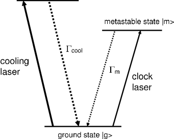
Figure 1: Transitions involved in the cooling and probing of an ion for a frequency standard. In practice, the cooling scheme may involve several lasers because of a possible hyperfine structure and/or a possible decay towards other metastable states. In most cases, $\Gamma_{cool}$ is of the order of 20 MHz whereas $\Gamma_{m}$ is of the order of 1 Hz.

The light scattered by the cooling transition is also used for detection of the ion. The probing of the clock transition by the local oscillator (a laser) is done by direct laser excitation. During this stage, all the preparation lasers are shut off. After excitation of the clock transition, the cooling lasers are switched on again. The quantum jump method [7] allows then to know if the atom is excited or not: the absence of fluorescence during the detection stage proves that the ion is ”shelved” in the metastable upper state whereas the presence of fluorescence signal means that the ion is still in the cooling cycle. Repetition of this measurement as a function of the clock laser frequency allows to measure the transition probability distribution. In the following, we discuss the laser characteristics and the maximum duration required for these various stages. The choice of the suited interrogation scheme is essential to minimize the Allan deviation.

2.1 Preparation and detection

We suppose the ion cooled to the Doppler limit in an RF-trap and located at the center of the trap, where the RF-trapping field is minimum and has little influence on the ion motion. Since the trap creates a quasi-harmonic potential, the motion of the ion is a superposition of oscillations at different frequencies due to the spatial anisotropy of the trapping device. If we suppose, for simplicity’s sake, that there is only one frequency of motion $\omega_{tr}/2\pi$ in the trap, the resulting atomic absorption spectrum is composed of a central frequency corresponding to the atomic transition $\omega_{0}/2\pi$ and sidebands separated by multiples of the motional frequency $(\omega_{0}\pm p\omega_{tr})/2\pi$, ($p$ integer). The sidebands are resolved if the width of each band is smaller than their mutual separation (the strong confinement condition [8]). This can be achieved in miniature traps with high motional frequencies ($\approx 1$ MHz) for all the narrow transitions considered as potential basis for frequency standards ($\Gamma_{m}\ll\omega_{tr}$, see figure 1). The intensity of each band $p$ in the spectrum depends on the oscillation amplitude $X$ of the ion in the trap like $J_{p}^{2}(kX)$ [8] where $k$ is the laser wavevector of the probed transition and $J_{p}$ the Bessel function of order $p$. As the functions $J_{p}^{2}(kX)$ have negligeable values when $p\gtrsim kX$, the smaller is $kX$, the less sidebands are visible. Laser-cooling the ion reduces its oscillation amplitude $X$ and thus the number of observable sidebands. A major step in the preparation of the ion is to access the Lamb-Dicke regime which is characterized by the reduction of the spectrum to few sidebands with a preponderant weight on the central frequency, this regime is reached if $kX\lesssim 1$.

The motion of the ion can be described by the occupation rate of the vibrational quantum levels, characterised by the mean vibrational quantum number $\left<n\right>$. This vibrational state can also be characterized from the classical point of view by an oscillation amplitude $X=\lambda_{tr}\sqrt{2\langle n\rangle+1}$, where the length $\lambda_{tr}=\sqrt{\hbar/2m\omega_{tr}}$ measures the size of the fundamental harmonic oscillator eigenstate $\left|n=0\right>$. This length depends on the atomic mass by $1/\sqrt{m}$ and, as an example, is equal to 11 nm for a calcium ion with $\omega_{tr}=2\pi\times 1$ MHz. The Lamb-Dicke condition $kX\lesssim 1$ can also be expressed by $k\lambda_{tr}\sqrt{2\langle n\rangle+1}\lesssim 1$. The Lamb-Dicke parameter $\eta=k\lambda_{tr}$ quantifies the ability for a system {ion+trap} to reach the Lamb-Dicke regime for a given transition. It is of the order of 0.1 for optical transitions (e.g. 0.095 for calcium’s clock transition in the trap taken as example).

In most cases, the frequency of motion in the trap is of the order of 1 MHz, whereas the atomic dipole transition used for laser cooling has a width $\Gamma_{cool}$ close to $2\pi\times 20$ MHz. On such broad transition ($\Gamma_{cool}/2\gg\omega_{tr}$) the Doppler limit for laser cooling can be approximated by the one of a free atom [8]. This leads to a thermal population of the harmonic trap vibrational levels characterized by $\langle n\rangle\simeq\Gamma_{cool}/2\omega_{tr}\simeq 10$. The Lamb-Dicke condition $\eta\sqrt{2\langle n\rangle+1}\lesssim 1$ is then fulfilled by the vibrational state reached by Doppler cooling ($\langle n\rangle\simeq 10$). This fulfillment sets the transition free of first order Doppler effect, while the second order Doppler effect is very small (see section 3.4). Furthermore the residual distribution of occupied vibrational levels still allows to drive coherent dynamics on the clock transition, as required for the interrogation schemes and confirmed numerically in the following. Since the time needed to reach the Doppler cooling limit is of the order of milliseconds while the optical pumping is faster than the millisecond, we can estimate $T_{prep}$ to 5 ms.

The duration required for the detection stage depends on the fluorescence signal collected on the strong dipole transition. For such transitions with a width of $\approx$ 20 MHz, one can expect at least 10⁴ counts per second (cps) over a stray light level of less than 100 cps. In these conditions, 10 ms-periods are sufficient to acquire enough signal to decide if the atom has been excited into the metastable state. As a consequence, 15 ms is a realistic estimation for the sum of the preparation and detection contributions to the cycle duration. To this minimum cycle duration must be added the excitation duration time $T_{exc}$. In the following subsection, we theoretically study the minimization of this probe time for different excitation schemes, assuming that the total cycle time $T_{c}=T_{exc}+15$ ms.

2.2 Choice of the excitation scheme

2.2.1 Evaluation of the minimum Allan deviation

The width $\Delta f$ of the observed transition and its signal to noise ratio depends on the laser excitation scheme. The choice of a high-frequency clock transition (in the optical domain) allows to reach smaller Allan deviations than the ones obtained on frequency standards in the microwave domain. Until now, the narrowest optical transition linewidth has been observed on a Hg⁺ ion [9] and has allowed to reach a relative frequency stability of $7\times 10^{-15}$ over 1 s averaging. In this article, we discuss possible excitation schemes independently of the ion implied. We introduce a reduced Allan deviation $\sigma^{\prime}=\sigma_{y}(\tau)\times f_{0}\sqrt{\tau}$ to quantify the expected frequency stability of the standard, keeping in mind that reduced Allan deviations between 1 and 10 have already been measured by several groups on lasers locked on atomic optical transitions.

Let $p_{m}$ be the probability for the ion to be in the metastable state once excited by the clock laser. The frequency of the transition, to which the clock laser will be locked, is deduced from the probability $p_{m}$ measured several times on the low and high frequency sides of the transition. This method of frequency discrimination requires the excitation probability $p_{m}$ to be around 0.5, where the slope of the probability distribution is the steepest and the frequency sensitivity is the highest.

Several sources of noise can limit the signal to noise ratio. Among these is the quantum projection noise [10] which is dominant once the technical noise has been reduced. The laser excitation creates a linear superposition of the ground ($\left|g\right>$) and metastable ($\left|m\right>$) states: $\sqrt{1-p_{m}}\left|g\right>+\sqrt{p_{m}}\left|m\right>$. During the detection stage, the atomic state is projected on one of these two atomic states. The variance of such a measurement is $p_{m}(1-p_{m})$ and causes a minimum noise $\sqrt{p_{m}(1-p_{m})}$ on the transition probability. This can be overcome by using squeezed states [11], which we do not consider here.

The maximum signal to noise ratio which can then be observed is

$$S/N=\sqrt{\frac{p_{m}}{1-p_{m}}}$$ (2)

which is maximum at resonance ($p_{m}=1$), where the frequency descrimination is unefficient. Thus, maximum frequency sensitivity and maximum signal to noise ratio are not compatible. Additionally, the finite upper-state lifetime leads to spontaneous decay which, for long excitation time, can reduce the maximum excitation probability. As a consequence, finding a compromise between all these incompatible requirements deserve precise studies of the excitation scheme.

Two excitation schemes have been experimentally tested by several groups: a single Rabi pulse or two temporally separated Ramsey pulses. The first one has been performed on Hg⁺ [2], In⁺ [12], Sr⁺ and Yb⁺[4], and the second one on Hg⁺ [2] and Sr⁺ [3]. In the following we discuss the principal features of each method and then compare them. To quantify the relative stability allowed by the discussed methods, we evaluate the reduced Allan deviation by

$$\sigma^{{}^{\prime}}=\sigma_{y}(\tau)\times f_{0}\sqrt{\tau}=\Delta f\sqrt{\frac{1-p_{m}}{p_{m}}}\sqrt{T_{c}}$$ (3)

For a high frequency sensitivity, we assume that the laser probes the transition on each side of the line, on the two frequencies corresponding to an excitation probability $p_{m}$ which is half of the maximum probability measured for zero detuning ($p_{m}$ can never exceed 1/2). The deduced $\Delta f$ when these probabilities are equal is then the FWHM of the experimental linewidth. The evolution of the density matrix of the two levels $\left|g\right>$ and $\left|m\right>$ is computed numerically. The atomic system is defined by the metastable lifetime $\tau_{m}$ fixed to 1 second ($\Gamma_{m}=1/\tau_{m}$), and it is driven by a Rabi pulsation $\Omega$. The motion of the ion is taken into account by a distribution of thermal vibrational levels, characterised by the mean vibration number $\left<n\right>$ and defined by $P(n)=\left(\left<n\right>/(1+\left<n\right>\right)^{n}$. The excitation probability $p_{m}$ is then an incoherent weighted sum of the probability for each vibrational level to be excited in the metastable state. For a given laser intensity, the Rabi pulsation from vibrational level $\left|n\right>\rightarrow\left|n\right>$ is proportional to $(1-\eta^{2}n)$ whereas it is proportional to $\eta\sqrt{n+1}$ for a $\left|n\right>\rightarrow\left|n+1\right>$ transition. We choose for $\eta$ the value of 0.095 calculated for a calcium ion in the trap described above. As the Doppler cooling leads to $\left<n\right>\simeq 10$, the excitation probability on the $\left|n\right>\rightarrow\left|n\right>$ band is higher than the $\left|n\right>\rightarrow\left|n\pm 1\right>$ bands so these last ones were neglected. If $\Omega$ is the Rabi pulsation for the $\left|n=0\right>\rightarrow\left|n=0\right>$ transition, $\Omega\times L_{n}(\eta^{2})$ is the one for the $\left|n\right>\rightarrow\left|n\right>$ transition, $L_{n}$ being the Laguerre polynomial [13]. The linewidth $\Gamma_{L}$ of the laser spectrum (FWHM) is taken into account by adding a source of decoherence equal to this width in the operator controlling the evolution of the density matrix [14]. For a laser detuning $\Delta_{L}$ and in the rotating wave approximation the density matrix evolves according to

$$\dot{\rho}_{gg} = -\dot{\rho}_{mm}=i\Omega/2\left(\rho_{gm}-\rho_{mg}\right)+\Gamma_{m}\rho_{mm}$$ (4)

$$\dot{\rho}_{gm} = -i\Delta_{L}\rho_{gm}+i\Omega/2\left(\rho_{gg}-\rho_{mm}\right)-\Gamma_{m}\rho_{gm}/2-\Gamma_{L}\rho_{gm}/2$$ (5)

2.2.2 Single pulse excitation

To avoid power broadening, the narrow transition can be experimentally observed if the Rabi pulsation $\Omega$ is smaller than the linewidth and the interrogation time longer than the lifetime. But because of the finite lifetime of the excited state, the maximum excitation probability is low and requires several seconds to be reached, reducing the relative stability even if the observed linewidth is close to the natural width. In an ideal context where the experiment is not limited by the laser stability, the calculations show that the smallest reduced Allan variance is reached with a single pulse which should last at least 1 s and drive the transition with $\Omega$ of the order of $2\times\Gamma_{m}$. With today’s laser stability a cycle time of a few secondes for a single measure seems not realistic. We rather consider excitation schemes with durations inferior to 1 second, since a cycle has to be repeated several times before a signal can be built up to counteract on the frequency of the local oscillator.

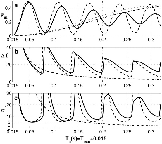
Figure 2: Calculations of the reduced relative stability $\sigma^{{}^{\prime}}$ (c), from the probability at half maximum $p_{m}$ (a) and the width $\Delta f$ (Hz) (b) of the excitation probability profile, for an increasing excitation time $T_{exc}$ ($T_{c}=T_{exc}+0.015$ s). This stability is calculated for a metastable lifetime $\tau_{m}=1/\Gamma_{m}=1$ s and a single Rabi pulse ( $\Omega=10\Gamma_{m}$ or $\Omega=100\Gamma_{m}$ ) for two thermal vibrational states characterised by $\left<n\right>=0$ and $\left<n\right>=10$. Dotted line: $\Omega=10\Gamma_{m}$ and $\left<n\right>=0$, dash-dotted line: $\Omega=10\Gamma_{m}$ and $\left<n\right>=10$, broken line: $\Omega=100\Gamma_{m}$ and $\left<n\right>=0$, solid line: $\Omega=100\Gamma_{m}$ and $\left<n\right>=10$. On (b) and (c), the dotted and dash-dotted line are almost superimposed and only one curve is plotted on the graph.

In figure 2, are plotted the excitation probability at half maximum $p_{m}$ , the full width at half maximum $\Delta f$ and the reduced stability as defined by equation (3), versus the cycle time $T_{c}=T_{exc}+$15 ms, assuming a single Rabi pulse. These curves reflect Rabi oscillations, which show maximum excitation probability for $T_{exc}=(2q+1)\pi/\Omega$ ($q$ integer). For $T_{exc}=2q\pi/\Omega$, the excitation probability is minimum on resonance and shows some maximum for other detunings. The computed FWHM has then no physical significance, which is not relevant here as a clock is never operated with this excitation duration. The interesting feature is the minimum of the reduced Allan variance observable for the shortest $T_{exc}$. Two cases with different Rabi pulsation $\Omega$ ($\Omega=10\Gamma_{m}$ and $\Omega=100\Gamma_{m}$) are compared in figure 2. For both cases, excitation probability and full width at half maximum are computed for an ion whose oscillatory motion corresponds to the Doppler cooling limit ($\left<n\right>=10$) or to the fundamental vibrational state ($\left<n\right>=0$). The first result to mention is that the first minima of the reduced Allan variance are identical for these two vibrational states, for the chosen Rabi pulsation. It confirms that Doppler cooling is sufficient for state preparation. The results shown in figure 2 suggest that the discrepancy between the $\left<n\right>=10$ and the $\left<n\right>=0$ vibrational state increases with the pulse duration. We have checked that in the case of the short pulses we consider in the following, the results are nearly the same for these two vibrational distributions and thus, from now on, only the cases concerning $\left<n\right>=0$ are dealt with.

To illustrate the influence of the strength of the Rabi pulsation in figure 2, the excitation is driven by $\Omega=10\times\Gamma_{m}$ and $\Omega=100\times\Gamma_{m}$. In the first case, the minimum reduced Allan deviation is close to 1 but requires an excitation of more than 300 ms. In the second case, the first minimum is reached for a cycle duration of 50 ms, but this shortening of the cycle duration is paid by an increase of $\sigma^{{}^{\prime}}$ equal to 4.5. This trend is general and a further increase of the Rabi pulsation leads to an increase of the minimum Allan deviation as well as a decrease of the required cycle time.

We now take into account the effect of a finite laser linewidth on the minimum reduced Allan deviation and compare the value computed for a laser as broad as the atomic transition ($\Gamma_{L}/2\pi=0.2$ Hz) to the one computed with a 20 Hz broad laser (FWHM). In this latter case, the performances of the clock are greatly reduced first by the reduction of the excitation probability and second by the broadening of the observed transition. The first drawback can be overcome by the increase of the Rabi pulsation but this is paid by a further increase of the transition broadening. As a consequence, for a given laser linewidth and a given metastable lifetime, there is an optimal Rabi pulsation which results in a minimum reduced Allan deviation. This is illustrated in figure 3 where for $\Gamma_{L}/2\pi=20$ Hz, $\sigma^{{}^{\prime}}$ is minimum ( $\sigma^{{}^{\prime}}$=12.4) for $100\times\Gamma_{m}\lesssim\Omega\lesssim 125\times\Gamma_{m}$ and a cycle time of 40 ms, whereas for $\Gamma_{L}/2\pi=0.2$ Hz, $\sigma^{{}^{\prime}}$ is minimum for $\Omega\simeq 4\Gamma_{m}$ and is then equal to 1.7 but for a cycle time of 625 ms. In the case of the broadest laser linewidth, these results confirm the intuitive idea that for optimum stability, the pulse length $T_{exc}$ is limited by the laser linewidth $T_{exc}\Gamma_{L}\simeq\pi$ and that the Rabi pulsation is then approximately set by the resonant $\pi$-pulse condition $\Omega T_{exc}\simeq\pi$. When the laser linewidth is comparable to the transition natural width ($\Gamma_{L}/2\pi=0.2$ s^-1), the optimum stability is reached for a shorter excitation time $T_{exc}\Gamma_{L}(\Gamma_{m})\simeq 0.6$ and a Rabi pulsation under the resonant $\pi$-pulse condition $\Omega T_{exc}\simeq 2.5$, which could not be dedeuced from the intuitive concept.

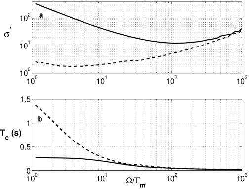
Figure 3: (a): Minimum reduced Allan deviation and (b): cycle duration $T_{c}$ required to reach this minimum versus the Rabi pulsation. Computation done for a metastable lifetime $\tau_{m}=1/\Gamma_{m}=1$ s and a single Rabi pulse by a laser of width $\Gamma_{L}$ (FWHM), with an ion in the vibrational ground state ($\left<n\right>=0$). Broken line: $\Gamma_{L}/2\pi=0.2$ Hz and solid line: $\Gamma_{L}/2\pi=20$ Hz.

2.2.3 Comparison with Ramsey interferometry

The introduction of the separated fields method or Ramsey interferometry [15] was soon followed by breakthroughs in high resolution spectroscopy and is expected to overcome the limitations met with single pulse excitation. With this method the line profile is recorded after two pulses of duration $T$ such as $\Omega T=\pi/2$, separated by a free evolution time $T_{free}$. When the laser detuning is scanned, the profile shows Ramsey fringes resulting from an interference pattern and for short enough pulse duration (or a high enough Rabi pulsation), the width of the central fringe is equal to $1/2T_{free}$ and is then independent from the Rabi pulsation. For a chosen pulsation $\Omega$, the evolution of $p_{m}$, $\Delta f$ and $\sigma^{{}^{\prime}}$ does not show oscillations with $T_{c}$ , like for a single Rabi pulse. $\sigma^{{}^{\prime}}$ takes very high values for short $T_{c}$ and decreases toward a limit for longer $T_{c}$. This limit depends on the choice of the pulsation $\Omega$.

When the width of the laser is taken into account by the relaxation it causes on the coherence, for a given Rabi pulsation, the reduced Allan deviation decreases for increasing free evolution time until it reaches critical time where the width of the laser broadens the line. This behaviour results in a minimum of the reduced Allan deviation reached for this critical cycle time and depending on the laser linewidth and the Rabi pulsation. For increasing Rabi pulsation $\Omega$, this minimum Allan deviation decreases towards a limit which depends very few on the laser linewidth as it varies by less than a factor of 2 over the whole range of the considered linewidth ( $0.1\leq\Gamma_{L}/2\pi\leq 100$ Hz). This is made possible by the short interaction time with the laser, allowed by a strong Rabi pulsation $\Omega$. In the case where the experiment is not limited by the available laser power, $\Omega$ must be chosen to reach a minimum Allan deviation close to the limit but also to cause a negligeable light-shift on the atomic levels. This light-shift is evaluated in section 3.3 and our calculations and numerical computations show that a Rabi pulsation $\Omega=1000$ s^-1 allows to reach the Allan deviation limit to better than 1% and to cause a negligeable light-shift.

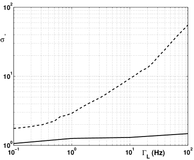
Figure 4: Minimum reduced Allan deviation versus the laser linewidth $\Gamma_{L}/2\pi$ (Hz), for a metastable lifetime $\tau_{m}=1/\Gamma_{m}=1$ s. The dashed line shows the minimum achievable reduced deviation with a single Rabi pulse (the cycle time and Rabi pulsation are computed to minimize $\sigma^{{}^{\prime}}$) . The solid line shows the minimum deviation achievable with a two Ramsey pulses excitation for a fixed Rabi pulsation of $1000\Gamma_{m}=$1000 s^-1 .

Figure 4 shows this minimum reduced Allan deviation for a laser linewidth from 0.1 Hz to 100 Hz (FWHM), compared with the one reached with a Rabi excitation scheme, where the best $\Omega$ and $T_{c}$ are found to reach the minimum Allan deviation, like explained in figure 3. The minimum Allan deviation expected for a narrow laser (0.1 Hz) for a Ramsey excitation scheme is 1.06 and for a Rabi scheme is 1.76. These values are very close to each-other but their evolution with the width of the laser is very different in the two cases. As shown in figure 4, for a Rabi excitation scheme, the minimum Allan deviation increases with the laser linewidth to reach $\sigma^{{}^{\prime}}=55$ for $\Gamma_{L}/2\pi=100$ Hz whereas it reaches 1.48 for a Ramsey scheme with the same laser linewidth. This evolution illustrates the great advantage of Ramsey two separated pulses excitation over a Rabi single pulse.

To give an insight of how such performances are reached, the excitation probability profiles calculated for the conditions giving the minimum Allan deviation for a 0.1 Hz laser linewidth are shown in figure 5.

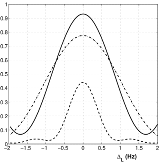
Figure 5: Excitation profile leading to minimum Allan deviation for a laser linewidth $\Gamma_{L}=0.1$ (Hz), for a metastable lifetime $\tau_{m}=1$ s. Solid line : profile reached for two Ramsey pulses, with $\Omega=1000\Gamma_{m}$ and $T_{c}=313$ ms. Dashed and dot-dashed line : profiles reached for a single Rabi pulse, two configurations lead to the same $\sigma^{{}^{\prime}}=1.76$: $\Omega=2\Gamma_{m}$ and $T_{c}=1.093$ s (dashed line) and $\Omega=7\Gamma_{m}$ and $T_{c}=392$ ms (dot-dashed line).

For a Ramsey scheme and the chosen Rabi pulsation of 1000 s^-1, the optimum cycle time is 313 ms and results in a 1.76 Hz wide profile ($\Delta f$) with $p_{m}=0.465$. For a single pulse, the minimum Allan deviation can be reached by two different Rabi pulses. One with $\Omega=2$ s^-1 and lasting 1.093 s gives rise to a narrow ($\Delta f=0.86$ Hz) but few excited profile ($p_{m}=0.22$). Another one with $\Omega=7$ s^-1 lasting 392 ms leads to a broader profile ($\Delta f=2.28$ Hz) with higher excitation ($p_{m}=0.39$). These three profiles illustrate the compromise required between high excitation probability and narrow linewidth to reduce the Allan deviation. They show that different conditions can reach this compromise. In any case, the Ramsey excitation scheme results in Allan deviation smaller than for a Rabi scheme. Furthermore, this method has the advantage of keeping low deviation even for laser linewidth broader than the transition.

2.2.4 Influence of the metastable level lifetime

We have computed the minimum reduced Allan deviation for different metastable level lifetimes $\tau_{m}$, for a very narrow laser ($\Gamma_{L}/2\pi=0.1$ Hz) and excitation by two Ramsey pulses with $\Omega=1000$ s^-1 as this value allows to reach the limit of the Allan deviation. The results are summarized in table 1. The computed Allan deviations are very close for all the ion optical frequency standard candidates (between 1.4 and $5.9^{-15}/\sqrt{\tau}$) confirming quantitatively the prediction that optical frequency standard will overtake the performances of existing microwave standards in the long run.

Table 1: Minimum Allan deviation expected for different optical frequency standard candidates, computed with a very narrow laser ($\Gamma_{L}/2\pi=0.1$ Hz) and two Ramsey pulses with $\Omega=1000$ s^-1.

atom	$\tau_{m}$ (s)	$\lambda$ (nm)	$\sigma^{{}^{\prime}}_{mini}$	$\sigma_{y}(\tau)$
In+	0.2	236	1.78	$1.4^{-15}/\sqrt{\tau}$
Ca+	1.15	729	1.05	$2.5^{-15}/\sqrt{\tau}$
Hg+	0.08	282	2.78	$2.6^{-15}/\sqrt{\tau}$
Sr+	0.4	674	1.40	$3.1^{-15}/\sqrt{\tau}$
Yb+	0.05	436	4.04	$5.9^{-15}/\sqrt{\tau}$

2.2.5 Summary

First, our studies confirm that a Ramsey excitation scheme is more appropriate than a Rabi one to take full advantage of very narrow atomic transition in the goal of building a frequency standard. They also show that the finite laser linewidth implies an optimum cycle time for a given Rabi pulsation, which can not be deduced intuitively from this linewidth as it ranges from $T_{c}=120$ ms for the shortest metastable lifetime listed on table 1 ($\tau_{m}=0.05$ s) to 312 ms for the longest metastable level lifetime $\tau_{m}=1.15$ s (Ca⁺). The Allan deviation expected for a Ca⁺ standard is $2.5^{-15}/\sqrt{\tau}$ which ranks well among the other candidates for optical frequency standard.

3 Frequency standard accuracy and precision

Besides the frequency stability, the other relevant parameters defining the quality of a frequency standard are its accuracy and its precision. The standard frequency may be shifted from the atomic resonance value by any interaction of the atom with external fields. If this shift is constant, it only reduces the standard accuracy but not its precision. If this shift varies in time or can not be evaluated exactly, the precision is reduced also. As these effects contribute to the uncertainty of the future frequency standard, all the interactions of the ion with its surrounding must be controlled to minimise and/or to maintain any shift of the clock frequency. We evaluate these shifts for a calcium ion in order to choose the best internal state and prepare an environment for which these shifts are minimum.

The ground state $\left|g\right>$ of the calcium ion is $\left|S_{1/2}\right>$ and the metastable state $\left|m\right>$ is $\left|D_{5/2}\right>$ with a measured lifetime of $1152\pm 23$ ms [16] which leads to a natural width for the clock transition of $138\pm 3$ mHz. We require that during the excitation of the transition by the clock laser, all other lasers are shut off. This assures that there are no light-shifts of the levels $S_{1/2}$ and $D_{5/2}$ caused by the cooling lasers. The other major effects that can shift the standard frequency are due to the local magnetic and electric fields and to the intensity of the clock laser itself. In the Lamb-Dicke regime, the Doppler effect shifts the line only by its second order contribution. We first focus on the Zeeman effect as it governs the choice of the isotope and atomic sublevels used for the standard.

3.1 Zeeman effect

To avoid any uncontrolled or time-varying shifts, the frequency standard must be made as independent as possible of environmental conditions. The first order Zeeman effect can be eliminated by the use of atomic Zeeman sublevels with no projection of the total moment on the magnetic field. This can be realised by the use of an isotope with a half integer nuclear spin. The most abundant one (0.135% in a natural sample) is ⁴³Ca⁺ with a nuclear spin 7/2.

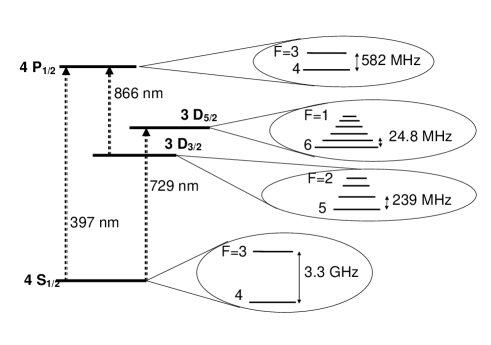
Figure 6: Hyperfine structure of the levels involved in the preparation, excitation and detection of ⁴³Ca⁺ ($I=7/2$) [17, 18].

The hyperfine structure of this isotope can be found on figure 6. Alternatively, the first order Zeeman effect could be eliminated on the ⁴⁰Ca⁺ transition by cancellation between $\left|S_{1/2},m=1/2\right>\rightarrow\left|D_{5/2},m=1/2\right>$ and $\left|S_{1/2},m=-1/2\right>\rightarrow\left|D_{5/2},m=-1/2\right>$. The exact cancellation of the first order Zeeman effect to better than one hertz requires a stability of the magnetic field better than $10^{-4}\mu$T for at least a few seconds, which seems difficult to realise. As a consequence the use of the odd isotope appears to be the easiest solution to eliminate the first order Zeeman shift from the standard frequency.

The second order Zeeman shift depends on the choice of the hyperfine sublevels. We calculate these shifts by searching the eigenvalues of the Zeeman Hamiltonian for the $\left|F,m_{F}\right>$ states. The Zeeman shift of the fundamental hyperfine levels $\left|S_{1/2},F=3{\rm\ or\ }F=4,m_{F}=0\right>$ are at least 2 orders of magnitude smaller than the shift of the metastable hyperfine levels $\left|D_{5/2},F=1,...,6,m_{F}=0\right>$ and are not relevant for the choice of the level. Figure 7 shows the quadratic Zeeman shifts for the different hyperfine levels of $D_{5/2}$ for sublevels $m_{F}=0$.

Figure 7: Zeeman shift of the metastable hyperfine sublevels of $D_{5/2}$ versus the magnetic field, for Zeeman sublevel $m_{F}=0$.

These curves illustrate the great variation of these shifts with the hyperfine sublevel. Depending on the level involved, the second order Zeeman effect can be as large as 98.04 Hz/$\mu$T² for $F=1$ or reduced to -9.05 Hz/$\mu$T² for $F=6$ (see figure 7). This last level should be used as a basis to reduce the second order Zeeman effect of the standard. As the $\left|S_{1/2}\right>\rightarrow\left|D_{5/2}\right>$ transition is electric-quadrupole, the selection rules $\Delta F=0,\pm 1,\pm 2$ imply that the fundamental sublevel involved in the standard should be $\left|S_{1/2},F=4,m_{F}=0\right>$.

To eliminate the uncertainty due to the Zeeman effect, the local magnetic field must be kept on the 0.1 $\mu$T level. A controlled magnetic field is still needed to split all the Zeeman sublevels and to be able to select the $\left|m_{F}=0\right>\rightarrow\left|m_{F}=0\right>$ transition. The two closest transitions $\left|S_{1/2},4,\pm 1\right>\rightarrow\left|D_{5/2},6,\pm 1\right>$ are split apart by $\pm 3.5$ kHz/$\mu$T. So a magnetic field of 0.1 $\mu$T allows to isolate the $m_{F}=0\rightarrow m_{F}=0$ transition and can be measured by the observation of these neighbouring transitions. Nevertheless, such a magnetic field may not be sufficient to maintain a high level of scattered light by the atomic system, as observed for other ions under study [4]. But it is possible to recover a high level signal by spinning of the laser polarisation [19, 4] and we do not consider, at this level, this reduction of the signal as a limitation. Without any magnetic field applied, the local field caused by the earth and the experimental setup is of the order of $10^{-4}$ T and such fields can be produced by 1 A in Helmholtz coils. Furthermore, magnetic field fluctuations of 0.2 $\mu$T over one day have been observed in an unshielded environnement [20]. As a consequence, in a thermalized and shielded environnement, it is technically possible with standard current supplies of 1 A stabilized to the mA level, to compensate for the already existing magnetic field and to add the desired magnetic field of $0.1\pm 0.05\mu$T. In these conditions, the frequency uncertainty due to the Zeeman effect is

$$B=0.1\pm 0.05\ \mu{\rm T}\rightarrow\delta f_{Z}=-0.09\pm 0.09\ {\rm Hz}$$ (6)

Indeed, it is possible to prepare the atomic system in the $\left|S_{1/2},F=4,m_{F}=0\right>$ state thanks to the property of dipole transition that forbids $\left|F,m_{F}=0\right>\rightarrow\left|F,m_{F}=0\right>$ transitions. After the cooling stage, two lasers polarised parallel to the magnetic field ($\Delta m_{F}=0$) and resonant with the $\left|S_{1/2},F=4{\rm\ and\ }F=3\right>\rightarrow\left|P_{1/2},F=4\right>$ transitions optically pump the system in the $\left|S_{1/2},F=4,m_{F}=0\right>$ state in few microseconds, then ready for the probe stage. Actually, the cooling and optical pumping stage are not so simple due to a possible decay from $P_{1/2}$ to $D_{3/2}$ level (see figure 6), whose lifetime is the same order of magnitude as $D_{5/2}$ and so requires three repumping lasers, to empty the possibly occupied $F=3,4,5$ levels. If the repumping lasers are $\sigma(=\sigma^{+}+\sigma^{-})$ polarised, the cooling and optical pumping remains efficient, as long as the three repumping lasers’ detunings are different from the two cooling ones, to avoid dark resonances [21] and as long as their polarization is spun to prevent pumping into dark states [19]. With its very low natural abundance, the use af such an isotope is technically challenging, but it has been shown that photoionisation processes allow to create ⁴³Ca⁺ ions even from a non-enriched calcium sample [22].

3.2 Interaction with DC electric fields and their gradients

The second order Stark effect shifts the standard frequency through the coupling of the levels $S_{1/2}$ and $D_{5/2}$ to all the other atomic levels by electric dipole interaction with any DC or slowly varying electric fields. These fields also shift the $D_{5/2}$ level by the coupling of its electric quadrupole moment to any electric field gradient. In a usual miniature spherical trap, the confining electric field has no static component, oscillates at a frequency of the order of 10 MHz and its shape in the center can be very well approximated by a quadrupole. In the exact center of the trap there should be no oscillating field but an oscillating field gradient. However, in a real Paul trap, patch potentials deform the harmonic potential well created by the RF field. They separate the minimum potentiel point from the zero RF-field point and static bias voltages have to be applied in the three directions to make these two points meet again and reduce any static field to less than V/cm. This step is required to be able to cool an ion to the Doppler limit and to reach the Lamb-Dicke regime [23] and can lead to an increase of the static electric field gradient. Such gradient can realistically reach 1V/mm on 1 mm (the typical diameter of a Paul-Straubel trap). The local electric field is then the sum of the quadrupole oscillating field that traps the ion, the bias static field lower than V/cm and the isotropic field radiated by the vessel considered as a blackbody. Since the frequencies of this radiated field are far below the optical resonance of Ca⁺, the field can be taken into account by its mean-square value averaged over all the blackbody spectrum, whose value is given by [24]

$$\left<E_{BB}^{2}\right>=831.9^{2}\left(\frac{T}{300}\right)^{4}$$ (7)

in (V/m)² with $T$ in Kelvin. At room temperature, this field overtakes the static bias field resulting from compensation of patch potentials. Nevertheless, it can be drastically reduced by cooling the vessel, a thermalization at 77 K sets this field below the level of V/cm, comparable to the bias static one.

Thanks to a symmetry property of the second order Stark Hamiltonian (which behaves like a second order tensor), the Stark shift of $S_{1/2}$ is independent of the hyperfine level and Zeeman sublevel. As a consequence, it is also independent of the polarisation of the electric field and behaves like a scalar (this property is true for any level with $J<1$). An electric field couples the ground state $4S_{1/2}$ to all the $nP_{1/2}$ and $nP_{3/2}$ levels but in the fact, the sum of the oscillator strength on $4P_{1/2}$ and $4P_{3/2}$ is already equal to 1 [25] and there is no point taking into account other couplings to $n>4$ levels. The second order Stark shift on $4S_{1/2}$ is then easily evaluated to $-9.5$ mHz/(V/cm)².

The Stark effect on the $D_{5/2}$ level can be split into a scalar term, independent on $F$ and $m_{F}$ and a tensorial part, depending on these two quantum numbers and on the angle $\theta$ between the electric field and the magnetic field defining the quantification axis. The sum of all the oscillator strengths of the transitions between $3D_{5/2}$ and $nP_{3/2}(n\geq 4)$, $nF_{5/2}(n\geq 4)$ and $nF_{7/2}(n\geq 4)$ is only 0.48 (according to the Harvard database [25]), suggesting that there are other couplings with levels belonging to the continuum. Then our evaluation can only be a rough estimation, but it gives a correct order of magnitude. We find $-3.9$ mHz/(V/cm)² for the scalar part and $+2.1$ mHz/(V/cm)${}^{2}\times(3\cos^{2}\theta-1)/2$ for the tensorial part and associate an uncertainty as high as the value itself to take into account that there are missing couplings. The total frequency shift due to DC-Stark effect is then

$$\delta f_{S}(S_{1/2} \rightarrow D_{5/2},F=6,m_{F}=0)$$ (8)

$$= 5.6(\pm 4)+2.1(\pm 2)\times\left(\frac{3\cos^{2}\theta-1}{2}\right)\ \ {\rm mHz/(V/cm)}^{2}$$

At room temperature, the DC Stark shift is mainly due to the isotropic radiated field and is therefore

$$\delta f_{S}(S_{1/2}\rightarrow D_{5/2},F=6,m_{F}=0)=0.39(\pm 0.27)\ \ {\rm Hz}$$ (9)

If the vessel is cooled to 77 K, the contribution of the radiated field is of the same order as the bias static field so its direction is unknown and its amplitude of the order of 1 V/cm. Such a field induces an uncertainty on the frequency of

$$\delta f_{S}(77K)(S_{1/2}\rightarrow D_{5/2},F=6,m_{F}=0)\leq 12\ \ {\rm mHz}$$ (10)

As for the coupling of the electric quadrupole moment of the $3D_{5/2}$ state to any electric field gradient, it depends on the hyperfine level, its Zeeman sublevel and on the shape as well as on the symmetry axis of the electric potential [26]. The coupling strength is due to a non spherical repartition of the electronic charge density and depends on the atomic orbitals of the considered level. The quadrupole moment $\Theta(3D_{5/2})$ of the fine structure state can be defined as [26]:

$$\Theta(3D_{5/2})=-\frac{e}{2}\left<3D_{5/2},\ m_{J}=\frac{5}{2}|3z^{2}-r^{2}|3D_{5/2},\ m_{J}=\frac{5}{2}\right>$$ (11)

This is calculated by considering the electronic orbital of $3D_{5/2}$ as pure $3d$ without any mixing with other electronic orbitals. For a single electron atom [27]

$$\Theta=\frac{e}{2}\left<r^{2}\right>\frac{2J-1}{2J+2}$$ (12)

In our case:

$$\Theta(3D_{5/2})=\frac{2e}{7}\left<r^{2}\right>_{3d}$$ (13)

In [26], the Cowan code is used to compute $\left<r^{2}\right>_{5d}$ for Hg⁺. A good enough and simple estimation of $\left<r^{2}\right>$ in alkali like ion is provided by the quantum defect method [28] which gives a simple relation between the energy $E_{nl}$ of the electronic level and an effective quantum number $n^{*}(l)$ by

$$E_{nl}=-\frac{\widetilde{Z}^{2}}{n^{*2}(l)}a.u.,\widetilde{Z}=Z-N+1$$ (14)

$\left<r^{2}\right>_{3d}$ can then be calculated using the one-electron orbital properties, with $\widetilde{Z}$ and $n^{*}$ instead of $Z$ and $n$. This method gives for Ca⁺

$$\left<r^{2}\right>_{3d}=6.6a_{0}^{2}$$ (15)

where $a_{0}$ is the Bohr radius. The energy shift of the hyperfine sublevel $\left|F=6,m_{F}=0\right>$ of $3D_{5/2}$ is

$$\delta E=\frac{7}{11}\left(\frac{2e}{7}\left<r^{2}\right>_{3d}\right)\left(\frac{1}{2}\frac{\partial^{2}V}{\partial x^{2}}\right)\Pi$$ (16)

where $\Pi$ is a geometrical factor equal to $(3\cos^{2}\beta-1)$ if the field has a quadrupole symmetry ($V\propto x^{2}+y^{2}-2z^{2}$), $\beta$ being the angle between its symmetry axis and the magnetic field defining the quantization axis [26]. The frequency shift of the standard transition under investigation is then

$$\delta f=8.1\times 10^{-7}\left(\frac{1}{2}\frac{\partial^{2}V}{\partial x^{2}}\right)\Pi\ \ \ {\rm Hz}$$ (17)

The hyperfine level has little influence on this shift as, for exemple, for the level $F=2$, 7/11 is replaced by 17/35. With the expected gradient of 1 V/mm over 1 mm, the uncertainty induced by this effect reaches the hertz level, which is high compared to the width of the clock transition in Ca⁺. Any modification of the patch potential, due for exemple to the ion creation process, alters this shift and reduces the reproductibility of the standard. Still, this effect can be eliminated by averaging the transition frequency measured with the magnetic field along three perpendicular directions, as the geometrical $\Pi$ factor is then averaged to zero [26]. The remaining uncertainty will then depend on the precision of the angle setting between the three measurements. This precision depends a lot on the vessel design and experimental setup, and it seems difficult to estimate this uncertainty as long as we have not performed the experiment. Nevertheless, other authors [29] have projected to reduce by 50 the uncertainty induced by this shift and we assume that a reduction by a factor of 10 is readily achievable, which sets the uncertainty induced by the quadrupole effect to $\pm 0.1$ Hz. At this point, it is important to mention that in spherical traps, the field gradient is inferior to the one in linear traps, due to the confining geometry. As a consequence, in order to minimize the shift induced by the gradient a spherical trap is preferred to a linear trap.

3.3 Interaction with AC electric fields

During the excitation of the clock transition, only one laser is applied. It can still cause an AC-Stark shift (or light-shift) of $S_{1/2}$ and $D_{5/2}$ by coupling them to $P_{1/2}$ and $P_{3/2}$ by dipole interaction or by coupling them to other Zeeman sublevels of $D_{5/2}$ and $S_{1/2}$ by quadrupole interaction (the coupling with $D_{3/2}$ is far less strong). The first two couplings produce a shift proportional to the laser intensity $I_{729}$ equal to $1.1\times 10^{-4}\times I_{729}$ Hz. The laser intensity required to produce the highest Rabi pulsation of 1000 $s^{-1}$ considered in part 2.2.3 on the $\left|S_{1/2},\ 4,\ 0\right>\rightarrow\left|D_{5/2},\ 6,\ 0\right>$ transition is 0.75 $\mu$W/mm², which leads to a light-shift caused by dipole coupling equal to 0.08 mHz, which is however negligeable compared to the natural width of the transition.

Light-shifts of a few kHz due to quadrupole interaction with other Zeeman sublevels have been measured on ⁴⁰Ca⁺ isotope [30]. In these experiments Rabi pulsations of 1 MHz were used with laser detunings of the order of 1 MHz. Here we calculate this shift in the context of the clock transition excitation for a Rabi pulsation equal to $1000$ s^-1 and a magnetic field of 0.1 $\mu$T. The frequency detuning required to probe the clock transition depends on the laser linewidth and on the Rabi pulsation used, and is of the order of 1 Hz. By chosing $\pm 10$ Hz for this detuning the light-shift is then not underestimated. We find an effect equal to $\pm 6$ mHz decreasing to $\pm 0.06$ mHz if the magnetic field is 1 $\mu$T. The sign depends on the sign of the detuning. Two reasons make this effect very small: the small Rabi pulsation considered for such experiments and the small detuning required to probe the two sides of the transition (of the order of a few Hz). With such small detuning, the couplings of $\left|S_{1/2},4,0\right>$ with $\left|D_{5/2},6,2\right>$ and with $\left|D_{5/2},6,-2\right>$ compensate each other (and vice-versa for $\left|D_{5/2},6,0\right>$ with $\left|S_{1/2},4,\pm 2\right>$). Nevertheless, with the laser power and magnetic field values planned for the optical clock realisation, this effect overtakes the ones induced by dipole couplings.

3.4 Second order Doppler shift

The second order Doppler effect shifts the frequency transition by

$$\frac{\delta f_{D}}{f_{0}}=-\frac{\left<v^{2}\right>}{2c^{2}}$$ (18)

With an oscillating ion, cooled to the Doppler limit, the velocity of the ion can be written like $v=V_{0}\cos(\omega_{tr}t+\phi)$ and $\left<v^{2}\right>=V_{0}^{2}/2$. This mean-square velocity is calculated by $V_{0}=\omega_{tr}X$ and $X=\lambda_{tr}\sqrt{2\langle n\rangle+1}$ (cf 2.1). With the values chosen in 2.1, the velocity amplitude $V_{0}$ is equal to 0.32 m/s leading to a second order Doppler relative shift given by

$$\frac{\delta f_{D}}{f_{0}}=-2.8\times 10^{-19}$$ (19)

In the case of the Ca⁺ clock transition ($f_{0}=4.11\times 10^{14}$ Hz) , the absolute shift is $0.11$ mHz, which is negligeable in the reduction of the clock precision. This calculation confirms that Doppler laser cooling is sufficient also to reduce the second order Doppler effect to negligeable values.

3.5 Uncertainty budget

Table 2 gives the uncertainty budget expected for an atomic clock based on ⁴³Ca⁺. At room temperature, and with the considered magnetic field, the major source of frequency shift and uncertainty is the Stark effect induced by the radiated electromagnetic field. This effect is drastically reduced in a vessel cooled to 77 K and then the major source of uncertainty becomes the coupling with the field gradient through the quadrupole moment of $D_{5/2}$ which limits the ultimate precision of the clock. It can be compensated by measuring the frequency with three perpendicular directions of magnetic field. Nevertheless, the obtained precision will depend on the design of the experimental setup and the ability to control the directions of the laser propagation and magnetic field. The projections made for all these major systematic shifts show that an atomic frequency standard based on $\left|S_{1/2},\ 4,\ 0\right>\rightarrow\left|D_{5/2},\ 6,\ 0\right>$ of ⁴³Ca⁺ can reach an uncertainty of $4\times 10^{-16}$, with room for improvement by better compensation of the quadrupole shift and better stabilization of the magnetic field.

Table 2: Uncertainty budget for the frequency transition of $\left|S_{1/2},\ 4,\ 0\right>\rightarrow\left|D_{5/2},\ 6,\ 0\right>$ in ⁴³Ca⁺

effect	fields/conditions	shift (Hz)@ 300 K	@ 77 K
second order Zeeman effect	0.1 $\mu$T	$-0.09\pm 0.09$	$-0.09\pm 0.09$
Stark effect	radiated and bias static field	$+0.39\pm 0.27$	$\leq$ 0.012
$D_{5/2}$ coupled to the field gradient	1 V/mm2	$\pm 0.1$	$\pm 0.1$
AC Stark effect @ 729 nm	0.75 $\mu$W/mm2, 0.1 $\mu$T	$\pm 0.006$	$\pm 0.006$
second order Doppler effect	ion cooled to the Doppler limit	$-1\times 10^{-4}$	$-1\times 10^{-4}$
global shift and uncertaintity		+0.3 $\pm 0.4$	-0.09 $\pm$ 0.19
relative shift and uncertaintity		$+7(\pm 9)\times 10^{-16}$	-2 ($\pm$ 4)$\times 10^{-16}$

4 Conclusion

We have presented a theoretical evaluation of the ultimate performances that can be expected from an optical frequency standard based on an electric quadrupole transition of a trapped single ⁴³Ca⁺ ion. We studied its stability through its Allan deviation, assuming that the signal to noise ratio would be limited by the quantum projection noise. Our results show that a frequency instability of $\approx 2.5\times 10^{-15}/\sqrt{\tau}$ can be expected. We also show that a Ramsey excitation scheme allows to take advantage of a very narrow transition, even with a laser broader than this transition, whereas this is not possible with a single Rabi pulse. The minimum Allan deviation is also computed for the other ions which are candidates for an optical frequency standard and Calcium ranks well within this list.

In a second time, all the systematic frequency shifts have been estimated and the environmental conditions studied in order to minimize the frequency uncertainty. This minimization is limited by the precision reached in the successive orientation of 3 mutually perpendicular magnetic fields to compensate the coupling of the $D_{5/2}$ quadrupole with a field gradient. A technical challenge for the future optical frequency standard will be to point these three perpendicular magnetic fields and to reduce the field gradient. In this context, a miniature spherical trap is more appropriate than a linear one to a frequency standard. Our projections show that with a first step alignement and a cooled vessel, a standard based on $\left|S_{1/2},\ 4,\ 0\right>\rightarrow\left|D_{5/2},\ 6,\ 0\right>$ of ⁴³Ca⁺ can reach an uncertainty of $4\times 10^{-16}$, an order of magnitude smaller than the most precise actual microwave frequency standard [31].

Acknowledgement

The authors would like to thank F. Schmidt-Kaler for very helpful discussions. Our project has been supported by the Bureau National de Métrologie.

References

- [1] E. Braun, J. Helmcke, special feature: Quantum measurement standards, (Eds) Meas. Sci. Technol. 14 (2003) 1159.
- [2] R. Rafac, B. Young, J. Beall, W. Itano, D. Wineland, J. Bergquist, Sub-decahertz ultraviolet spectroscopy of 199Hg+, Phys. Rev. Lett. 85 (12) (2000) 2462.
- [3] L. Marmet, A. Madej, Optical Ramsey spectroscopy and coherence measurements of the clock transition in a single trapped Sr ion, Can. J. Phys. 78 (2000) 495.
- [4] P. Gill, G. Barwood, H. Klein, G. Huang, S. Webster, P. Blythe, K. Hosaka, S. Lea, H. Margolis, Trapped ion optical frequency standards, Meas. Sci. Technol. 14 (2003) 1174.
- [5] M. Eichenseer, A. Y. Nevsky, C. Schwedes, J. von Zanthier, H. Walther, Toward an indium single-ion optical frequency standard, J. Phys. B 36 (2003) 553.
- [6] C. Champenois, M. Knoop, M. Herbane, M. Houssin, T. Kaing, M. Vedel, F. Vedel, Characterization of a miniature Paul-Straubel trap, Eur. Phys. J. D 15 (2001) 105.
- [7] H. Dehmelt, Radiofrequency spectroscopy of stored ions I: storage, Advances in Atomic and Molecular Physics 3 (1967) 53–72.
- [8] D. Wineland, W. Itano, Laser cooling of atoms, Phys. Rev. A 20 (4) (1979) 1521.
- [9] S. Diddams, T. Udem, J. Bergquist, E. Curtis, R. Drullinger, L. Hollberg, W. Itano, W. Lee, C. Oates, K. Vogel, D. Wineland, An optical clock based on a single trapped 199Hg+ ion, science 293 (2001) 825.
- [10] W. Itano, J. Bergquist, J. Bollinger, J. Gilligan, D. Heinzen, F. Moore, M. Raizen, D. Wineland, Quantum projection noise: population fluctuations in two level systems, Phys. Rev. A 47 (5) (1993) 3554.
- [11] D. Wineland, J. Bollinger, W. Itano, D. Heinzen, Squeezed atomic states and projection noise in spectroscopy, Phys. Rev. A 50 (1) (1994) 67.
- [12] T. Becker, J. v.Zanthier, A. Y. Nevsky, C. Schwedes, M. Skvortsov, H. Walther, E. Peik, High-resolution spectroscopy of a single In+ ion: progress towards an optical frequency standard, Phys. Rev. A 63 (2001) 051802R.
- [13] C. Blockley, D. Walls, H. Risken, Europhys. Lett. 17 (1992) 509.
- [14] C. Cohen-Tannoudji, Frontiers in laser spectroscopy, Les Houches 1975, North-Holland, 1977, p. 58.
- [15] N. Ramsey, Molecular beams, Oxford, 1956.
- [16] M. Knoop, C. Champenois, G. Hagel, M. Houssin, C. Lisowski, M. Vedel, F. Vedel, Metastable lifetimes from electron-shelving measurements with ion clouds and single ions, Eur. Phys. J. D 29 (2003) 163.
- [17] F. Arbes, M. Benzing, T. Gudjons, F. Kurth, G. Werth, Precise lifetime determination of the ground state hyperfine structure splitting of 43Ca II, Z. Phys. D 31 (1994) 27.
- [18] W. Nörtershäuser, K. Blaum, K. Icker, P. Müller, A. Schmitt, K. Wendt, B. Wiche, Isotope shifts and hyperfine structure in the transitions in calcium II, Eur. Phys. J. D 2 (1998) 33.
- [19] D. Berkeland, M. Boshier, Destabilization of dark states and optical spectroscopy in Zeeman-degenerate atomic systems, Phys. Rev. A 65 (2002) 033413.
- [20] S. Bize, S. Diddams, U. Tanaka, C. Tanner, W. Oskay, R. Drullinger, T. Parker, T. Heavner, S. Jefferts, L. Hollberg, W. Itano, J. Bergquist, Testing the stability of fundamental constants with the 199Hg+ single ion optical clock, Phys. Rev. Lett. 90 (15) (2003) 150802.
- [21] G. Janik, W. Nagourney, H. Dehmelt, Doppler-free optical spectroscopy on the Ba+ mono-ion oscillator, J. Opt. Soc. Am. B 2 (8) (1985) 1251.
- [22] D. M. Lucas, A. Ramos, J. P. Home, M. J. McDonnell, S. Nakayama, J.-P. Stacey, S. C. Webster, D. N. Stacey, A. M. Steane, Isotope-selective photoionization for calcium ion trapping, Phys. Rev. A 69 (2004) 012711.
- [23] D. Berkeland, J. Miller, J. Bergquist, W. Itano, D. Wineland, Minimization of ion micromotion in a Paul trap, J. Appl. Phys. 83 (1998) 5025.
- [24] W. Itano, I. Lewis, D. Wineland, Shift of hyperfine splittings due to blackbody radiation, Phys. Rev. A 25 (2) (1982) 1233.
- [25] Kurucz, Atomic line database, cdrom 23, http://cfa-www.harvard.edu/amdata/ampdata/kurucz23/sekur.html (2003).
- [26] W. Itano, External-field shifts of the 199Hg+ optical frequency standard, J. Res. Natl. Inst. Stand. Technol. 105 (2000) 829.
- [27] I. Sobelman, Atomic spectra and radiative transitions, Springer-Verlag, 1992.
- [28] B. Bransden, C. Joachain, Physics of atoms and molecules, Longman scientific et technical, 1994.
- [29] P. Gill, G. Barwood, G. Huang, H. Klein, P. Blythe, K. Hosaka, R. Thompson, S. Webster, S. Lea, H. Margolis, Trapped ion optical frequency standards, EGAS 2003, Brussels, Physica Scripta T112 (2004).
- [30] H. Häffner, S. Gulde, M. Riebe, G. Lancaster, C. Becher, J. Eschner, F. Schmidt-Kaler, R. Blatt, Precision measurement and compensation of optical Stark shifts for an ion-trap quantum processor, Phys. Rev. Lett. 90 (2003) 143602.
- [31] A. Bauch, Caesium atomic clocks: function, performance and applications, Meas. Sci. Technol. 14 (2003) 1159.