Equivalence between focussed paraxial beams and the quantum harmonic oscillator

Abstract

The paraxial approximation to the scalar Helmholtz equation is shown to be equivalent to the Schrödinger equation for a quantum harmonic oscillator. This equivalence maps the Gouy-phase of classical wave optics onto the time coordinate of the quantum harmonic oscillator and also helps us understand the qualitative behavior of the field and intensity distributions of focused optical beams in terms of the amplitude and probability distributions of quantum harmonic oscillators and vice versa.

I Introduction

It is well known that in the limit of short wavelengths, wave optics can be reduced to ray-optics: Maxwell’s equations can be reduced to the eikonal equations of geometric optics.shortwavelength ; Born.Wolf.book Ray optics therefore is an emergent theory with limited applicability. The ray optical description of optical image formation is simple and satisfactory for many purposes. Indeed, if thin lens formulae apply and complications such as chromatic aberration can be neglected, the description is so simple that it is standard material in undergraduate physics education.textbook.thin.lens But optics requires a wave description when the characteristic length scales of a beam of light become comparable to its wavelength. Even when the thin lens formula appears to be applicable, a wave optical description becomes necessary where a focused light beam’s transverse extension shrinks to a point, for example, in all focal areas of a conventional imaging apparatus. Wave optics limits the resolution of point-images through aperture dependent point-spread functions.Born.Wolf.book ; textbook.thin.lens ; Saleh.Teich.book ; Siegman.book ; Haus.buch

We investigate the fundamental building blocks of general images: focused, monochromatic beams. Specifically, we consider focused beams in the paraxial approximation and assume that we can treat the polarization degrees of freedom separately so that we can apply the paraxial approximation to the scalar Helmholtz equation. Since a general image is described by a suitable mixture of coherent beams (of different frequencies, polarization, etc.) our considerations are of some generality. Beams that are not too strongly focused can typically be decomposed into a complete orthonormal set of modes that have a simple analytical description. The most widely used are the Hermite-Gaussian transverse electromagnetic modes (TEM-modes), which we will introduce in Sec. II. These modes are essentially suitably rescaled wave functions of a harmonic oscillator multiplied by phase factors arising from the specific geometry of the beam, see Eq. (4).Saleh.Teich.book ; Siegman.book ; Haus.buch This connection between coherent optical beams and harmonic oscillators is known, but it seems to be little appreciated that the two systems are isomorphic (but see Ref. Nienhuis, ). The amplitude of a focused paraxial beam corresponds to the amplitude of a quantum harmonic oscillator, the former’s intensity to the probability distribution of the latter, and the Gouy-phase of opticsFengOL01 assumes the meaning of time for the quantum harmonic oscillator.

We derive this equivalence by a transformation of the paraxial wave equation of optics into the Schrödinger equation for the quantum harmonic oscillator in Sec. III. We then give a few illustrative examples for this equivalence in Sec. IV, which will allow us to discuss some counterintuitive aspects of optical beam behavior.

II Hermite-Gaussian Beams: TEM-modes

General monochromatic TEM-beam modes in the paraxial approximation are solutions of the associated scalar Helmholtz equation for the electro-magnetic vector potential $\bf A$ propagating in vacuum at speed $c$ (with the dispersion relation, $\omega=ck$)Haus.buch

$$\nabla^{2}{\bf A}({\bf r},t)-\frac{1}{c^{2}}\frac{{\partial}^{2}{\bf A}({\bf r},t)}{\partial t^{2}}=0,$$ (1)

where ${\bf r}=(x,y,z)$ and $t$ describe position and time coordinates. A monochromatic beam with wave number $k$ travelling in the positive $z$-direction and linearly $x$-polarized is described by the vector potential ${\bf A}=(A_{x},A_{y},A_{z})$ whose only non-zero component is $A_{x}$ withHaus.buch

$$A_{x}({\bf r},t;k)=\psi({\bf r})\;e^{i(kz-\omega t)}.$$ (2)

If we insert this ansatz into the Helmholtz equation (1) and factor out the common plane wave phase factor $e^{i(kz-\omega t)}$, we obtain a differential equation for the field envelope $\psi({\bf r})$ alone:

$$0 = \frac{{\partial}^{2}\psi({\bf r})}{\partial x^{2}}+\frac{{\partial}^{2}\psi({\bf r})}{\partial y^{2}}+\frac{{\partial}^{2}\psi({\bf r})}{\partial z^{2}}+2ik\frac{{\partial}\psi({\bf r})}{\partial z}$$ (3a)

$$\approx \frac{{\partial}^{2}\psi({\bf r})}{\partial x^{2}}+\frac{{\partial}^{2}\psi({\bf r})}{\partial y^{2}}+2ik\frac{{\partial}\psi({\bf r})}{\partial z}.$$ (3b)

Equation (3b) represents the paraxial approximation; it is based on the observation that, for beams that are not too strongly focused (several wavelengths across), the $z$-dependence of the field derivative is primarily due to the plane wave factor $2ik$, which allows us to discard the dependence on $\partial\psi/\partial z$. When we perform the second derivative, the term $\partial^{2}\psi/\partial z^{2}$ is consequently assumed to be negligible.Haus.buch

The paraxial approximation significantly simplifies our task because it has the familiar transverse electromagnetic TEM_mn-modes $\psi_{mn}$ as solutions.Saleh.Teich.book ; Siegman.book ; Haus.buch They contain products of Gaussians and Hermite polynomials in the transverse beam coordinates $x$ and $y$, that is, the familiar harmonic oscillator wave functions $\varphi_{m}(\xi)=H_{m}(\xi)\exp(-\xi^{2}/2)/\sqrt{2^{m}m!\sqrt{\pi}}$, $(m=0,1,2,\ldots),$ and various phase factors,Saleh.Teich.book ; Siegman.book ; Haus.buch namely

$$\psi_{mn}({\bf r})=\frac{w_{0}}{w(z)}\varphi_{m}(\frac{\sqrt{2}\,x}{w(z)})\,\varphi_{n}(\frac{\sqrt{2}\,y}{w(z)})$$

$$\times\;e^{\frac{ik}{2R(z)}(x^{2}+y^{2})}\;e^{-i(m+n+1)\phi(z)}.$$ (4)

The relation that links the minimal beam radius $w_{0}$ with the Rayleigh range $b$ via the light’s wavelength $\lambda$ and wave number $k$ is given by $w_{0}=\sqrt{2b/k}=\sqrt{\lambda b/\pi}$. The beam radius (where the intensity has dropped to $1/e^{2}$ of the central intensity) at the distance $z$ from the beam waist obeys $w(z)=\sqrt{w_{0}^{2}(1+z^{2}/b^{2})}$, and for large $z$ implies the expected amplitude decay of a free wave $\propto 1/|z|$ with a far-field opening angle $\arctan(\lambda/(\pi w_{0}))$.

The corresponding wave front curvature is described by the radius $R(z)=(z^{2}+b^{2})/z$, and the longitudinal Gouy-phase shiftSiegman.book ; Haus.buch follows

$$\phi(z)=\arctan(z/b)\;,$$ (5)

which varies most strongly at the beam’s focus. Note that the associated Gouy-phase factor $e^{-i(m+n+1)\phi(z)}$ depends on the order $n$ and $m$ of the mode functions. Different modes therefore show relative dephasing or mode-dispersion, particularly near the focus.

The vector potential $A_{x}$ of Eq. (2) describes a beam travelling in the positive $z$-direction (${\bf k}=k\hat{\bf z}$) and yields an electric field that is polarized in the $x$-direction with a small contribution in the $z$-direction due to the tilt of wave fronts off the beam axis.Haus.buch According to Maxwell’s equations in the paraxial approximation, that is, neglecting transverse derivatives, we find for the electric field vector,Haus.buch ($\hat{\bf x},\hat{\bf y},\hat{\bf z}$ are the unit-vectors and Re stands for the real part)

$${\bf E}({\bf r},t;{\bf k})=\mbox{Re}\big{\{}[\hat{\bf x}\omega\psi({\bf r})+\hat{\bf z}ic\frac{\partial\psi({\bf r})}{\partial x}]e^{i(kz-\omega t)}\big{\}}.$$ (6)

The associated instantaneous electrical intensity distribution isHaus.buch

$$I({\bf r},t)=\frac{\epsilon_{0}}{2}{\bf E}({\bf r},t)^{2}\approx\frac{\epsilon_{0}}{2}\;\omega^{2}\mbox{Re}\{A_{x}({\bf r},t)\}^{2}.$$ (7)

III Transformation to Harmonic Oscillator Schrödinger Equation

We have derived the paraxial approximation of the wave equation in Eq. (3) and found that the solutions, except for some phase factors and a coordinate rescaling in the arguments of the solutions, look like those of the quantum harmonic oscillators. We shall therefore now “undo” these various factors and transform the paraxial wave equation into Schrödinger’s equation to establish the isomorphism between both systems.

Figure 1: Plot of new coordinate lines $\xi=\mbox{constant}$ in the $xz$-plane.

Based on the shape of the solutions (4), we apply the following coordinate transformations $[x,y,z]\mapsto[\xi,\eta,\tau]$, which establishes new coordinate lines $\xi$ and $\eta$ that follow the focused beams’ hyperbolic flow lines (see Fig. 1)

$$x=\xi\frac{w(z)}{\sqrt{2}},\quad y=\eta\frac{w(z)}{\sqrt{2}}.$$ (8)

Because of Eq. (5), we let

$$z=b\tan(\tau),$$ (9)

where $\tau$ plays the role of time. If we use these new coordinates and the ansatz $\psi(x,y,z)=\Psi(\xi,\eta;\tau)e^{\frac{ik}{2R(z)}(x^{2}+y^{2})}/w(z)$ in the paraxial wave equation (3), we find after a lengthy but straightforward calculation

$$\Big{[}-{\frac{\partial^{2}}{\partial{\eta}^{2}}}-{\frac{\partial^{2}}{\partial{\xi}^{2}}}+{\eta}^{2}+{\xi}^{2}-2\,i{\frac{\partial}{\partial\tau}}\Big{]}\Psi(\xi,\eta;\tau)=0,$$ (10)

which is the Schrödinger equation for the harmonic oscillator. The units are $\hbar=m=\Omega=1$, where $m$ is the mass and $\Omega=2\pi/T$ is the resonance frequency of the harmonic oscillator. We have established the equivalence between focused beams and harmonic quantum oscillators.

Note that the $z$-coordinate $z=(-\infty,\infty)$ in the optical case was transformed to time $\tau=(-\pi/2,\pi/2)$ in the harmonic oscillator case, whereas the role of time in the optical case has no analog in the harmonic oscillator case because we had to factor out the plane wave phase factor $e^{i(kx-\omega t)}$. In other words, the isomorphism we established links the beam’s envelope amplitude $\psi(x,y,z)$ with a two-dimensional harmonic oscillator wave function $\Psi(\xi,\eta;\tau)$.

IV Examples: Single-mode and Two-mode Profiles

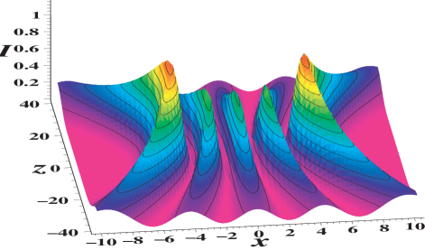
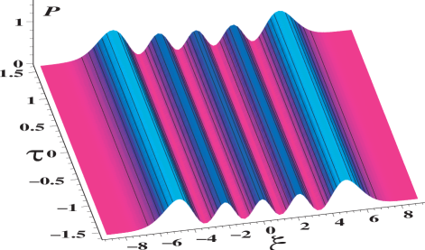
Figure 2: Top: Contour plot of the time-averaged intensity $I(x,0,z)$ of a field with mode structure TEM₄₀, namely, $\varphi_{4}(\sqrt{2}x/w(z))\varphi_{0}(\sqrt{2}y/w(z))$, around the beam focus $(0,0,0)$; Rayleigh length $b=20\lambda$. In this and all other figures of optical beams the intensity is in arbitrary units and the coordinates are in units of $\lambda$. Bottom: Contour plot of the evolution of the probability distribution of a one-dimensional quantum harmonic oscillator with wave function $\Psi(\xi)=\varphi_{4}(\xi)$.

For simplicity, we will now consider one-dimensional beam patterns. We choose the $y$-mode to be the zero-mode, and thus concentrate on the behavior in the transverse $x$-direction only, that is, we investigate the beams in the $xz$-plane. For easy comparison, we depict focused beams with a beam parameter of $b=20\lambda$. Our first example is that of a single TEM₄₀-beam, plotted in Fig. 2; we next consider a more interesting case, a two-mode superposition of TEM-modes 30 and 40 (see Fig. 3).

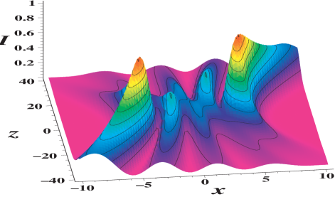
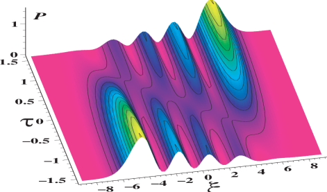
Figure 3: Average intensity $I(x,0,z)$ of a field with mode structure $[\varphi_{4}(\sqrt{2}x/w_{0})-i\varphi_{3}(\sqrt{2}x/w_{0})]\varphi_{0}(\sqrt{2}y/w_{0})$ at the beam focus $z=0$; $b=20\lambda$. Bottom: Contour plot of the evolution of the non-normalized probability distribution of a one-dimensional quantum harmonic oscillator with wave function $\Psi(\xi;0)=\varphi_{4}(\xi)-i\varphi_{3}(\xi)$.

For the two-mode superposition in Fig. 3 we can clearly see the interference between modes $\varphi_{3}$ and $\varphi_{4}$ at work and how it leads to the redistribution of the intensity from one beam edge to the other, thus inverting the transverse beam profile about the beam axis. This intensity redistribution is ultimately due to the mode-dispersive effect of the Gouy-phase factor $e^{i(m+n+1)\phi}$ in the optical case and the time phase factor $e^{i(m+1/2+n+1/2)\Omega t}$ for the two-dimensional harmonic oscillator. Note that a beam that is focused only in one transversal direction (using a cylindrical lens rather than a spherical one) corresponds to a one-dimensional harmonic oscillator,FengOL01 because in this case the Gouy-phase factor is $e^{i(m+1/2)\phi}$ and corresponds to a one-dimensional harmonic oscillator phase factor $e^{i(m+1/2)\Omega t}$. Clearly, both systems evolve through half an oscillation period ($t=-T/4,\ldots,T/4$. (Remember, the Gouy-phase (5) varies from $-\pi/2$ to $\pi/2$.)

We know from ray optics that images become inverted at the focus. Here we see how this image inversion arises through the action of the Gouy-phase. In the language of the harmonic oscillator, it corresponds to half an oscillation $[-\pi/2,\pi/2]$ or swinging to the “other” side.

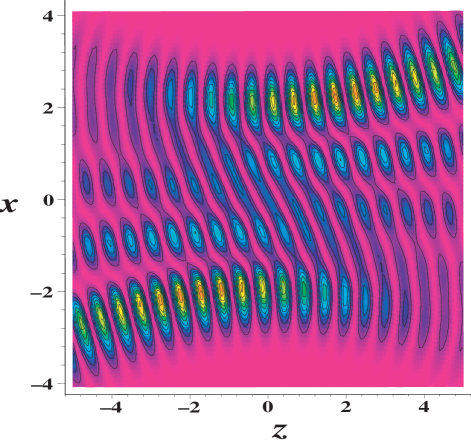
Figure 4: Instantaneous intensity $I(x,0,z;0)$ of a field with mode structure $[\varphi_{4}(\sqrt{2}x/w_{0})-i\varphi_{3}(\sqrt{2}x/w_{0})]\varphi_{0}(\sqrt{2}y/w_{0})$ at the beam focus $z=0$. For clarity, a smaller beam parameter of $b=5\lambda$ was chosen.

To gain further insight, we plot the beam’s instantaneous intensity distribution $I(x,0,z;0)$ in Fig. 4. It can clearly be seen that the relative phase of $90^{\circ}$ between modes 4 and 3 tilts the wave fronts, and the action of the Gouy-phase “transports” the beam’s envelope across the focus.

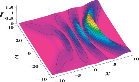
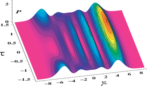
Figure 5: Average intensity $I(x,0,z)$ of a field with mode structure $[\varphi_{4}(\sqrt{2}x/w_{0})+\varphi_{3}(\sqrt{2}x/w_{0})]\varphi_{0}(\sqrt{2}y/w_{0})$ at the beam focus $z=0$; $b=20\lambda$. Bottom: Contour plot of the evolution of the non-normalized probability distribution of a quantum harmonic oscillator with wave function $\Psi(\xi;0)=\varphi_{4}(\xi)+\varphi_{3}(\xi)$.

Similarly to the case discussed in Fig. 3, but at first seemingly less intuitively, we can also have a scenario where the harmonic oscillator starts out with an average position at the beam center, then swings up to one side and falls back to the center. In wave optical terms this scenario corresponds to a field with a symmetric far-field distribution that is asymmetric at the focus and becomes symmetric in the far-field on the other side, this is illustrated in Fig. 5.

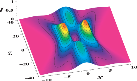
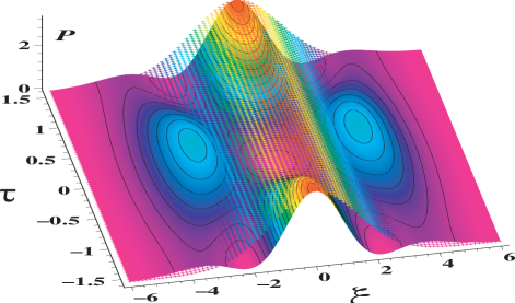
Figure 6: Average intensity $I(x,0,z)$ of a field with mode structure $[\varphi_{0}(\sqrt{2}x/w_{0})+\varphi_{2}(\sqrt{2}x/w_{0})]\varphi_{0}(\sqrt{2}y/w_{0})$ at the beam focus $z=0$; $b=20\lambda$. Bottom: Contour plot of the evolution of the non-normalized probability distribution of a quantum harmonic oscillator with wave function $\Psi(\xi;0)=\varphi_{0}(\xi)+\varphi_{2}(\xi)$. For comparison this distribution is overlayed by the non-normalized distribution for the ground state wave function $\varphi_{0}(\xi)$ alone. It shows that the superposition state $\Psi$ is very tightly confined in the $\xi$-direction, see text.

It also is possible to create a beam that, in oscillator language, starts out in the center and swings to either side to fall back to the center forming an annulus with a dark center at the beam’s focus (see Fig. 6). It also can be viewed as a beam that is overly focused in the far field. Then, according to Heisenberg’s uncertainty principle $\Delta(x)\Delta(p_{x})\geq\hbar/2$, such a spatially strongly localized harmonic oscillator carries a large momentum uncertainty. The bottom of Fig. 6 displays the harmonic oscillator ground state together with the superposition of modes 0 and 2. Clearly the superposition is spatially more confined than the ground state, and its Fourier transform reveals a large spread, namely, a central peak and two momentum peaks that are displaced from zero. In other words, this superposition describes a harmonic oscillator that “explodes” sideways and then swings back to the center. The seemingly counterintuitive formation of a dark center at the focus becomes easy to understand. Its two-dimensional analog is the optical bottle beam observed very recently.optical-bottles The latter is formed from a superposition of Laguerre-Gaussian modes 0 and 2, and thus carries basically the same structure in a cylindrical geometry as our example of Fig. 6 in the $xz$-plane.

A possible technical implementation of the patterns discussed here is sketched in Fig. 7 and has recently been demonstrated experimentally.ole.glasgow For further details on experimental implementations using computer-generated holograms, consult Refs. optical-bottles, ; ole.glasgow, ; computer.hologram, . The field profiles sketched here should be useful for optical manipulation techniques as well.ole_jopa05

Figure 7: Sketch of possible implementation using a laser, two lenses $L_{1}$ and $L_{2}$, and a suitable hologram $H$. The hologram modulation of the laser beam is mapped into the focal region $F$ of lens $L_{2}$. Formally, the transverse field profile in its focal plane is the Fourier-transform of the hologram-pattern.

V Conclusion

Focused beams cannot be described by ray optics in their focal region. Therefore an intuitive understanding of the wave optical behavior of a coherent, focused beam with transverse intensity modulation is desirable. It is shown that the paraxial wave equation is equivalent to the Schrödinger equation of a two-dimensional harmonic oscillator. This equivalence is used to show how the passage of a beam through its focus can be understood in terms of the behavior of a harmonic oscillator evolving through half a period.

In particular, the inversion of a focused beam’s far-field intensity pattern about the beam axis, upon passage through the focus, is described in terms of a harmonic oscillator swinging to the “other” side, and the formation of a bottle beam is explained by the behavior of a constricted beam pattern that corresponds to a harmonic oscillator fanning outward and recollapsing.

- (1) H. Goldstein, Classical Mechanics (Addison-Wesley, Reading, MA, 1981).
- (2) M. Born and E. Wolf, Principles of Optics (Pergamon, London, 1970).
- (3) R. A. Serway, Physics for Scientists and Engineers (Saunders, New York, 1990); M. Alonso and E. J. Finn, Physics (Addison-Wesley, Reading, MA, 1992).
- (4) B. E. A. Saleh and M. C. Teich, Photonics (Wiley, New York, 1991).
- (5) A. E. Siegman, Lasers (Oxford University Press, Oxford, 1986). Note that Gouy’s name is misspelled as ”Guoy” in this reference.
- (6) H. A. Haus, Electromagnetic Noise and Quantum Optical Measurements (Springer, Heidelberg, 2000).
- (7) G. Nienhuis and L. Allen, “Paraxial wave optics and harmonic oscillators,” Phys. Rev. A 48, 656–665 (1993); G. Nienhuis and J. Visser, “Angular momentum and vortices in paraxial beam,” J. Opt. A: Pure Appl. Opt. 6, S248–S250 (2004).
- (8) S. Feng and H. G. Winful, “Physical origin of the Gouy phase shift,” Opt. Lett. 26, 485–487 (2001).
- (9) J. Arlt and M. J. Padgett, “Generation of a beam with a dark focus surrounded by regions of higher intensity: The optical bottle beam,” Opt. Lett. 25, 191–193 (2000).
- (10) O. Steuernagel, E. Yao, K. O’Holleran, M. Padgett, “Observation of Gouy-phase-induced intensity changes in the beam focus,” unpublished.
- (11) M. Reicherter, T. Haist, E. U. Wagemann, and H. J. Tiziani, “Optical particle trapping with computer-generated holograms written on a liquid-crystal display,” Opt. Lett. 24, 608–610 (1999).
- (12) O. Steuernagel, “Coherent transport and concentration of particles in optical traps using varying transverse beam profiles,” J. Opt. A: Pure Appl. Opt. (in press); O. Steuernagel, Optical Particle Manipulation Systems, UK patent application No 0327649.0 (2003).