Data-driven derivation of the turbulent energy cascade generator

Abstract

Within the framework of random multiplicative energy cascade models of fully developed turbulence, expressions for two-point correlators and cumulants are derived, taking into account a proper conversion from an ultrametric to an Euclidean two-point distance. The comparison with two-point statistics of the surrogate energy dissipation, extracted from various wind tunnel and atmospheric boundary layer records, allows an accurate deduction of multiscaling exponents and cumulants. These exponents serve as the input for parametric estimates of the probabilistic cascade generator.

I Introduction

The inertial-range dynamics of fully developed turbulent flows reveals an ubiquitous multiscale character, driven by large-scale forcing on one end and controlled by fluid viscosity and small-scale dissipation on the other. For the intermediate scale range, the underlying Navier-Stokes equations do not disclose any other distinguishing length scales, thus suggesting a picture of a scale-invariant inertial-range dynamics MON71 ; FRI95 ; comment . This scale-invariance should reflect itself in the scaling of structure functions, which are moments of velocity increments constructed from the measured velocity data. However, measured structure functions in shear flows seem to show only an approximate multiscaling character, even at the largest accessible Reynolds numbers, where the large-scale and the dissipation scale are separated by five orders of magnitude ARN96 ; SRE97 ; SREE98 . The reason for this distortion of scaling seems to be the sensitivity of structure functions to the mean shear that is inevitably present in most natural flows at high Reynolds numbers. While schemes have been proposed to account for these effects arad ; SREE98 , it has been demonstrated recently CLE03 that the lowest-order two-point correlation function of the surrogate energy dissipation of a high-Reynolds-number atmospheric boundary layer reveals a far more convincing power-law scaling over the entire inertial range, without having to resort to shear corrections of the sort needed for structure functions. This finding suggests that the phenomenological picture of the self-similar turbulent energy cascade may contain more truth than previously anticipated. Consequently, it is reasonable to reexamine simple empirical energy cascade models and extend to a higher level the comparison between the models and experimental data. This is the purpose of the paper.

Random multiplicative cascade processes (RMCP) present a particularly simple geometrical picture of the energy cascade FRI95 and are a natural archetype for multiscaling. In their binary version, for example MS , they introduce a hierarchy of length scales $l_{j}=L/2^{j}$ and a random multiplicative cascade generator is used to transport the energy flux from the integral scale $L$ through the inertial range scales $L\geq l_{j}\geq\eta$ down to the dissipation scale $\eta=L/2^{J}$. Referring to the ultrametric branching structure of binary RMCPs, $N$-point correlation functions of arbitrary order have been calculated analytically with generating function techniques GRE95 ; GRE96 ; GRE98a ; GRE98b . In terms of the ultrametric two-point distance, which measures the number of cascade steps necessary to reach the last common branching, these models reveal rigorous multiscaling. However, in this form, the two-point RMCP statistics cannot be compared directly to quantities that can be extracted from the data because, from an experimentalist’s perspective, the two-point correlations are expressed as functions of the Euclidean two-point distance. In this respect, RMCPs are incomplete and have to be supplemented by model-dependent extensions, stating the conversion of the ultrametric to Euclidean statistics JOU02 ; EGG01 ; MEN90 . It may be expected that this unavoidable conversion will lead to some deviations from rigorous multiscaling of correlation functions for two-point distances within the inertial range. The challenge is to find the degree to which the theoretical, extended-RMCP, two-point correlation functions can match their experimental counterparts.

If this comparison is satisfactory, the two-point correlation statistics of the energy dissipation will allow for an unambiguous extraction of multiscaling exponents, these being related to moments of the RMCP generator. In addition, two-point cumulants of logarithmic energy dissipation EGG01 allow us to access properties of the cascade generator in another way. Taken together, reliable parametric estimations of the underlying cascade generator can then be given. This would be the best we can do to achieve a data-driven derivation of the turbulent energy cascade generator and to settle the question of whether the latter is bimodal SCH85 ; MEN87 , log-normal OBU62 ; KOL62 , log-stable KID91 ; SCH92 , log-infinite divisible SHE94 ; DUB94 ; SHE95 or another type of distribution. None of those prototype cascade generators has been directly derived from data.

Note that the breakup coefficients, sometimes called multipliers, have once been thought to represent a direct approach to derive the RMCP cascade generator from data CHAB92 ; SRE95 ; MOL95 ; PED96 ; NEL96 . In fact, generator-like scale-invariant distributions of breakup coefficients have been observed, but conditional distributions have been found to exhibit scale correlations. In a series of papers JOU99 ; JOU00 ; JOU02 these findings have been fully explained within ultrametric hierarchical RMCPs, once those are analyzed from an experimentalist’s perspective, including unavoidable small-scale resummation and restoration of spatial homogeneity via the ultrametric-Euclidean conversion. This work has demonstrated that cascade generators and distributions of breakup coefficients are not directly related.

The structure of this paper is as follows. Section II provides basic information about the two-point correlation of the lowest order for the surrogate energy dissipation in four fully developed turbulent flows—one atmospheric boundary layer and three wind-tunnel flows. This information serves to provide the needed guidance for the subsequent RMCP modelling of Sec. III, where analytic expressions for two-point correlators and cumulants are derived, taking into account the ultrametric-Euclidean conversion. More information on data analysis is provided in Sec. IV, leading in Sec. V to further comparisons between prototype distributions and experiments. As will also be demonstrated in this section, the extracted properties of the generator allow us to make parametric estimations of the RMCP cascade generator. A conclusion and outlook is given in Sec. VI.

II Data analysis I: basic facts on two-point statistics

We analyze four different data sets, three of which have been recorded in a wind tunnel PEA02 and the fourth in an atmospheric boundary layer DHR00 about 35 m above the ground. We will refer to them as w1, w2, w3 and a, respectively. Characteristic quantities of all data sets are summarized in Table 1. The Reynolds number $R_{\lambda}=\sqrt{\langle u^{2}\rangle}\lambda/\nu$ is based on the Taylor microscale $\lambda=\sqrt{\langle u^{2}\rangle/\langle(\partial u/\partial x)^{2}\rangle}$; $\nu$ is the kinematic viscosity and $u$ is the streamwise velocity component. Upon the application of the frozen flow hypothesis, the recorded time series were converted into one-dimensional spatial series. The energy spectra of all four records reveal more or less the typical $5/3$ slope in the inertial range. In contrast to wind-tunnel records, that from the atmospheric boundary layer reveals a white-noise behavior at very small scales; this noise, which comes from detailed electronic circuitry, has been removed by an appropriate Wiener filter. The energy dissipation was then calculated as the surrogate amplitude $\varepsilon=15\nu(\frac{du}{dx})^{2}$. Various tests were made to ensure that the effect of Wiener filtering were not consequential.

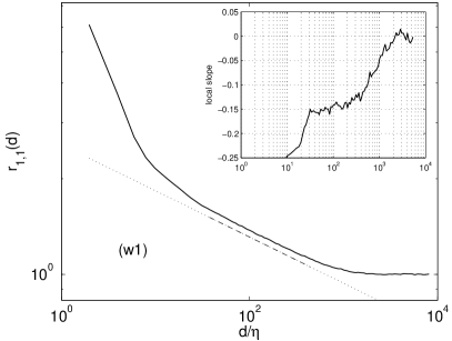
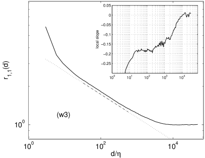
Figure 1: Two-point correlator $\langle\varepsilon(x+d)\varepsilon(x)\rangle/\langle\varepsilon(x)\rangle^{2}$ of the surrogate energy dissipation extracted from the records w1, w2, w3 and a. Power-law fits are indicated by the shifted broken straight lines. The inset figures illustrate the local slope.

Figure 1 illustrates the lowest-order two-point correlator $r_{1,1}(d=|x_{2}-x_{1}|)=\langle\varepsilon(x_{1})\varepsilon(x_{2})\rangle/(\langle\varepsilon(x_{1})\rangle\langle\varepsilon(x_{2})\rangle)$ sampled from the four different experimental records. Well inside the inertial range $\eta\ll d\ll L$ the two-point correlators reveal a power-law behavior $r_{1,1}\sim(L/d)^{\tau_{1,1}}$. Power-law fits are indicated by the shifted broken straight lines; see also the insets, where the local slopes are shown. The resulting scaling exponents are $\tau_{1,1}=0.15$ (w1), $0.14$ (w2), $0.18$ (w3) and $0.20$ (a). Note that there is a Reynolds number dependence of this exponent. This has been explored in greater detail elsewhere CLE03a .

For the records with the largest Reynolds number, there is a large scale range for which the two-point correlator exhibits a rigorous power-law scaling. However, with decreasing Reynolds number this scale range becomes smaller. As a rule of thumb, we observe that a good scaling range is confined between $d\approx 20{-}30\eta$ and $\approx 0.5L$. If we could understand precisely the deviations from the power-law scaling beyond this intermediate inertial range, a more satisfactory extraction of multiscaling exponents would be possible, especially for turbulent flows with moderate Reynolds numbers. In the small-distance $d\leq 20{-}30\eta$ region, however, the correlations observed exceed the power-law extrapolation; consult Fig. 1 again. As has been explained in Ref. CLE03 , this enhancement is a consequence of the unavoidable surrogacy of the experimentally measured energy dissipation. Without knowing the correct small-distance behavior based on the proper energy dissipation, a theoretical modelling of two-point correlations in the dissipative regime is not very meaningful. We are thus left to inspect only the remainder of the inertial range. Fortunately, this range is sufficiently large, especially for the atmospheric data.

At $d\approx L$, the two-point correlator has not yet converged to unity, which is its asymptotic value as $d{\to}\infty$. For all four data records inspected, the decorrelation length appears to be around $L_{\mathrm{dec}}\approx 4L$ and matches the length observed in the autocorrelation function of the streamwise velocity component. These findings suggest that the two-point correlator can be described as

$$r_{1,1}(20{-}30\eta<d\leq L_{\mathrm{dec}})=a_{1,1}\left(\frac{L_{\mathrm{dec}}}{d}\right)^{\tau_{1,1}}f_{1,1}(d/L_{\mathrm{dec}})\;.$$ (1)

For two-point distances $d$ much smaller than the decorrelation length the finite-size function converges to unity; that is, $f_{1,1}(d\ll L_{\mathrm{dec}})\to 1$. One goal of this paper is to qualitatively and quantitatively reproduce this functional form with an extended modelling based on random multiplicative cascade processes. This approach, which is the subject of the next section, naturally suggests a physical interpretation of the decorrelation length $L_{\mathrm{dec}}$.

III Two-point statistics of random multiplicative cascade processes

III.1 Binary random multiplicative cascade process

In its simplest form an RMCP employs a binary hierarchy of length scales $l_{j}=L_{\mathrm{casc}}/2^{j}$. In the first cascade step the parent interval of length $l_{0}=L_{\mathrm{casc}}$ is split into left and right daughter intervals, both of length $l_{1}$. In subsequent cascade steps, each interval of generation $0\leq j\leq J-1$ is again split into a left and right subinterval of length $l_{j+1}=l_{j}/2$. Once the dissipation scale $\eta=L_{\mathrm{casc}}/2^{J}$ is reached, the interval splitting stops and has resulted into $2^{J}$ spatially ordered intervals of smallest size $\eta$. It is convenient to label them as well as their ancestors according to the binary notation $\mathbf{\kappa}^{(j)}=\kappa_{1},\kappa_{2},\ldots,\kappa_{j}$. The label refers to the hierarchical position of an interval of generation $j$, where $\kappa_{i}=0$ or $1$ stands for the left or right interval, respectively.

The binary interval splittings go together with a probabilistic evolution of the energy-flux field. From generation $j$ to $j+1$ the field amplitudes propagate locally as

$$\Pi_{\mathbf{\kappa}^{(j)},0} = q_{\mathbf{\kappa}^{(j)},0}\Pi_{\mathbf{\kappa}^{(j)}}\;,$$

$$\Pi_{\mathbf{\kappa}^{(j)},1} = q_{\mathbf{\kappa}^{(j)},1}\Pi_{\mathbf{\kappa}^{(j)}}\;.$$ (2)

The two random multiplicative weights $q_{\mathrm{left}}=q_{\mathbf{\kappa}^{(j)},0}$ and $q_{\mathrm{right}}=q_{\mathbf{\kappa}^{(j)},1}$, with mean $\langle q_{\mathrm{left}}\rangle=\langle q_{\mathrm{right}}\rangle=1$, are drawn from a scale-independent bivariate probability density function $p(q_{\mathrm{left}},q_{\mathrm{right}})$, which is called the cascade generator. Initially, corresponding to $j=0$, the iteration (III.1) starts with a given large-scale energy flux $\Pi$, which might itself be a random variable fluctuating around its normalized mean $\langle\Pi\rangle=1$. After the last iteration $J-1\to J$, the energy-flux amplitude is interpreted as the amplitude $\varepsilon_{\mathbf{\kappa}^{(J)}}=\Pi_{\mathbf{\kappa}^{(J)}}$ of the energy dissipation supported at the interval of length $\eta$ at position $\mathbf{\kappa}^{(J)}$. As a result of (III.1), this amplitude is a multiplicative sum of the random weights, given by

$$\varepsilon_{\kappa_{1},\ldots,\kappa_{J}}=q_{\kappa_{1},\ldots,\kappa_{J}}q_{\kappa_{1},\ldots,\kappa_{J-1}}\cdots q_{\kappa_{1}}\Pi\;.$$ (3)

In the following we assume the cascade generator to be of the factorized form $p(q_{\mathrm{left}},q_{\mathrm{right}})=p(q_{\mathrm{left}})p(q_{\mathrm{right}})$ with identical statistics for the left/right variable. Of course, the factorization is not the most general ansatz but, as already pointed out in Ref. JOU00 , it represents a reasonable approximation: the turbulent energy cascade takes place in three spatial dimensions and calls for a three-dimensional RMCP modelling, respecting energy conservation. Since the measured temporal records come from one-dimensional cuts, the three-dimensional RMCP has to be observed in unity subdimension. Because of this, the RMCP appears to be non-conservative and the two multiplicative weights appear to be almost decorrelated and independent of each other.

III.2 Two-point correlators

Expressions for $N$-point moments $\langle\varepsilon(x_{1})^{n_{1}}\cdots\varepsilon(x_{N})^{n_{N}}\rangle$ are easily found. They can be calculated either by a straightforward approach or, more formally, by an iterative construction of the respective multivariate characteristic function GRE95 ; GRE96 ; a third and more elegant approach BIA99 makes use of the full analytic solution of the multivariate characteristic function for logarithmic cascade-field amplitudes GRE98a ; GRE98b . We simply state the results up to two-point correlations:

$$\left\langle\varepsilon(x_{1})^{n_{1}}\right\rangle = \left\langle q^{n_{1}}\right\rangle^{J}\left\langle\Pi^{n_{1}}\right\rangle\;,$$ (4)

$$\left\langle\varepsilon(x_{1})^{n_{1}}\varepsilon(x_{2})^{n_{2}}\right\rangle = \left\langle q^{n_{1}+n_{2}}\right\rangle^{J-D}\left\langle q^{n_{1}}\right\rangle^{D}\left\langle q^{n_{2}}\right\rangle^{D}\left\langle\Pi^{n_{1}+n_{2}}\right\rangle\;.$$ (5)

Here, the binary notation $\mathbf{\kappa}^{(J)}$ has been transformed into a spatial bin label $x=1+\sum_{j=1}^{J}\kappa_{j}2^{J-j}$, which runs over $1\leq x\leq 2^{J}$ in units of $\eta$. Two bins $x_{1}\equiv(\kappa_{1},\ldots,\kappa_{J-D},\kappa_{J-D+1},\ldots,\kappa_{J})$ and $x_{2}\equiv(\kappa_{1},\ldots,\kappa_{J-D},\kappa^{\prime}_{J-D+1},\ldots,\kappa^{\prime}_{J})$ are assigned an ultrametric distance $D$ once the first $J-D$ $\kappa$’s are identical and $\kappa_{J-D+1}\neq\kappa^{\prime}_{J-D+1}$. In other words, after $J-D$ common branches along the binary tree, the two bins separate into different branches.

For the extraction of scaling exponents

$$\tau_{n}=\log_{2}\langle{q^{n}}\rangle\;,$$ (6)

it is enough to consider the two-point statistics (5). In normalized form, the two-point correlators are found to scale perfectly as

$$r_{n_{1},n_{2}}(D) = \frac{\left\langle\varepsilon(x_{1})^{n_{1}}\varepsilon(x_{2})^{n_{2}}\right\rangle}{\left\langle\varepsilon(x_{1})^{n_{1}}\right\rangle\left\langle\varepsilon(x_{2})^{n_{2}}\right\rangle}$$ (7)

$$= \frac{\langle\Pi^{n_{1}+n_{2}}\rangle}{\langle\Pi^{n_{1}}\rangle\langle\Pi^{n_{2}}\rangle}\left(\frac{\left\langle q^{n_{1}+n_{2}}\right\rangle}{\left\langle q^{n_{1}}\right\rangle\left\langle q^{n_{2}}\right\rangle}\right)^{J-D}$$

$$= \frac{\langle\Pi^{n_{1}+n_{2}}\rangle}{\langle\Pi^{n_{1}}\rangle\langle\Pi^{n_{2}}\rangle}\left(\frac{L_{\rm casc}}{l_{D}}\right)^{\tau_{n_{1},n_{2}}}\;,$$

where $l_{D}=2^{D-1}\eta$ represents the characteristic two-bin distance corresponding to the ultrametric distance $D>0$ and

$$\tau_{n_{1},n_{2}}=\tau_{n_{1}+n_{2}}-\tau_{n_{1}}-\tau_{n_{2}}\;.$$ (8)

For an experimentalist, the expression (7) does not present an observable result. Different pairs of bins, all having an identical Euclidean distance $\eta{\leq}d{<}L_{\rm casc}$, do not have an unequivocal ultrametric distance. Depending on their position within the binary ultrametric cascade tree, the two bins might share a cascade history that is long (small $D$) or short (large $D$). Consequently, as an experimentalist analyzes the two-point statistics in terms of $d$, the ultrametric expression (7) has to be averaged over all $D$ that contribute to the same value of $d$. In order to perform this conversion from an ultrametric to an Euclidean distance and, by this means, to restore spatial homogeneity, we introduce the discrete conditional probability distribution

$$p(D|d)=\left\{\begin{array}[]{lcl}0&&(1{\leq}D{<}A{=}\lceil\log_{2}d\rceil)\\ 1-d2^{-D}&&(D{=}A)\\ d2^{-D}&&(A{<}D{\leq}J)\\ 0&&(J{<}D{<}\infty)\\ d2^{-J}&&(D{=}\infty)\end{array}\right.$$ (9)

of finding the ultrametric distance $D$ for a given Euclidean distance $d$ in units of $\eta$ EGG01 . This expression has been derived by employing the chain picture of independent cascade configurations; consult Fig. 2. It roughly goes as $p(D|d)\sim 2^{\log_{2}{d}-D}$. The sum $\sum_{D=0}^{J}p(D|d)=1-d2^{-J}$ does not add up to unity, since $p(\infty|d)=d2^{-J}$ represents the probability that the two bins belong to different $L_{\rm casc}$-domains.

Since the one-point statistics $\langle\varepsilon(x)^{n}\rangle=\langle\varepsilon(x+d)^{n}\rangle$ do not depend on the spatial index $x$, the ultrametric-Euclidean conversion of the normalized two-point correlator (7) leads to

$$r_{n_{1},n_{2}}(d{\neq}0) = \sum_{D=1}^{J}p(D|d)r_{n_{1},n_{2}}(D)+p(\infty|d)$$ (10)

$$= \frac{\langle\Pi^{n_{1}+n_{2}}\rangle}{\langle\Pi^{n_{1}}\rangle\langle\Pi^{n_{2}}\rangle}\left(1-\frac{d}{2^{A}}+\frac{d}{2^{A}}\left(2\frac{\langle{q^{n_{1}+n_{2}}}\rangle}{\langle{q^{n_{1}}}\rangle\langle{q^{n_{2}}}\rangle}-1\right)^{-1}\right)\left(\frac{\langle q^{n_{1}+n_{2}}\rangle}{\langle q^{n_{1}}\rangle\langle q^{n_{2}}\rangle}\right)^{J-A}$$

$$+\left(1-\frac{\langle\Pi^{n_{1}+n_{2}}\rangle}{\langle\Pi^{n_{1}}\rangle\langle\Pi^{n_{2}}\rangle}\left(2\frac{\langle{q^{n_{1}+n_{2}}}\rangle}{\langle{q^{n_{1}}}\rangle\langle{q^{n_{2}}}\rangle}-1\right)^{-1}\right)\frac{d}{2^{J}}\;.$$

This expression holds for every $\eta{\leq}d{\leq}L_{\rm casc}$. For $d{=}0$ and $d{>}L_{\rm casc}$ the normalized two-point density simply becomes $r_{n_{1},n_{2}}(d{=}0)=\langle\Pi^{n_{1}+n_{2}}\rangle\langle q^{n_{1}+n_{2}}\rangle^{J}/(\langle\Pi^{n_{1}}\rangle\langle q^{n_{1}}\rangle^{J}\langle\Pi^{n_{2}}\rangle\langle q^{n_{2}}\rangle^{J})$ and $r_{n_{1},n_{2}}(d{>}L_{\rm casc})=1$, respectively. The two-point density (10) does not reveal perfect scaling anymore. Usually the second term, scaling as $d/L_{\rm casc}$, is small when compared to the first term, except for $d{\approx}L_{\rm casc}$. The modulations, observed for the first term, are an artifact of the discrete scale invariance SOR98 of the binary random multiplicative cascade model implementation. In the following we will discard these modulations by first considering only dyadic distances $d_{m}=L_{\rm casc}/2^{m}$ with integer $0{\leq}m{<}J$, and then switching again to continuous $d$ by interpolating between the discrete $d_{m}$. The expression (10) then simplifies to

$$r_{n_{1},n_{2}}(d)=a_{n_{1},n_{2}}\left(\frac{L_{\rm casc}}{d}\right)^{\tau_{n_{1},n_{2}}}f_{n_{1},n_{2}}(d/L_{\rm casc}),$$ (11)

with

$$a_{n_{1},n_{2}}=\frac{\langle\Pi^{n_{1}+n_{2}}\rangle}{\langle\Pi^{n_{1}}\rangle\langle\Pi^{n_{2}}\rangle}\left(2\frac{\langle{q^{n_{1}+n_{2}}}\rangle}{\langle{q^{n_{1}}}\rangle\langle{q^{n_{2}}}\rangle}-1\right)^{-1}$$ (12)

and the finite-size scaling function

$$f_{n_{1},n_{2}}(d/L_{\rm casc})=1+\left(a_{n_{1},n_{2}}^{-1}-1\right)\left(\frac{d}{L_{\rm casc}}\right)^{1+\tau_{n_{1},n_{2}}}\;.$$ (13)

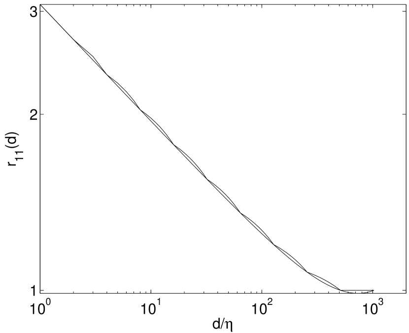
Figure 3: Comparison of the expressions (10) and (11) for the order $n_{1}=n_{2}=1$, showing that the log-oscillations inherent to (10) remain small. Parameters have been set as follows: $L_{\rm casc}/\eta=2^{10}$, $\tau_{2}=0.20$ and $\Pi=1$.

Figure 3 compares the expressions (10) and (11) for the order $n_{1}=n_{2}=1$.

The finite-size scaling function has the property $f_{n_{1},n_{2}}(d{\ll}L_{\rm casc})=1$ as long as the condition $1+\tau_{n_{1},n_{2}}\geq 0$ or, equivalently, $\langle q^{n_{1}+n_{2}}\rangle/(\langle q^{n_{1}}\rangle\langle q^{n_{2}}\rangle)>1/2$ is fulfilled. This is the case for all positive combinations $n_{1}\geq 0,n_{2}\geq 0$. However, combinations with negative orders do exist, for which the second term on the right hand side of (13) then dominates over the first term in the limit $d/L_{\rm casc}\to 0$. This implies that the normalized two-point density (11) asymptotically scales as $r_{n_{1},n_{2}}(d)\sim(L_{\rm casc}/d)^{-1}$, giving rise to the effective scaling exponents $\tau^{\rm eff}_{n_{1},n_{2}}=\sup\{-1,\tau_{n_{1},n_{2}}\}$. This scaling transition is again a pure consequence of the ultrametric-Euclidean conversion. More discussions on this subject can be found in Refs. MEN90 ; ONE93 ; BEN97 .

Upon studying the expression (13) more closely, we realize that two effects, ultrametric-Euclidean conversion and large-scale fluctuations, contribute to the finite-size scaling function. They have a tendency to cancel each other. Once we have

$$\frac{\langle\Pi^{n_{1}+n_{2}}\rangle}{\langle\Pi^{n_{1}}\rangle\langle\Pi^{n_{2}}\rangle}=2\frac{\langle q^{n_{1}+n_{2}}\rangle}{\langle q^{n_{1}}\rangle\langle q^{n_{2}}\rangle}-1\;,$$ (14)

the finite-size scaling function becomes $f_{n_{1},n_{2}}(d/L_{\rm casc})=1$ exactly, showing no $d$-dependence.

We also wish to point out an interesting mathematical observation following from the specific expressions (11)-(13). Since the finite-size scaling function (13) reveals the simple scaling behavior

$$\left(f_{n_{1},n_{2}}(d/L_{\rm casc})-1\right)\left(\frac{L_{\rm casc}}{d}\right)^{\tau_{n_{1},n_{2}}}\sim\left(\frac{d}{L_{\rm casc}}\right)^{\mu}$$ (15)

with $\mu=1$, we find

$$r_{n_{1},n_{2}}(d)-\frac{1}{\xi^{\mu}}r_{n_{1},n_{2}}(\xi d)=a_{n_{1},n_{2}}\left(1-\frac{1}{\xi^{\mu+\tau_{n_{1},n_{2}}}}\right)\left(\frac{L_{\rm casc}}{d}\right)^{\tau_{n_{1},n_{2}}}\;,$$ (16)

where the normalized two-point correlator with the rescaled two-point distance $\xi d$ has been subtracted from itself. As a function of the two-point distance $d$ this quantity exhibits a rigorous power-law behavior with scaling exponents $\tau_{n_{1},n_{2}}$, which is independent of the chosen rescaling parameter $\xi$ and is free of large-scale effects.

III.3 Two-point cumulants

Because experimental data yield limited statistics, the two-point correlation densities (11) will be restricted to lowest orders $1\leq n_{1}+n_{2}\leq 3$ or $4$. This limits us to indirect information on the cascade generator, namely the scaling exponents $\tau_{1},\tau_{2},\tau_{3}$ and, perhaps, $\tau_{4}$ of (6). In order to do better, we need to accumulate additional and complementary information. In fact, as proposed already in Ref. EGG01 , this can be achieved by switching to the logarithmic amplitude $\varepsilon(x)\to\ln\varepsilon(x)$, and from two-point correlation densities to two-point cumulants

$$C_{1,1}(x_{2}{-}x_{1}) = \left\langle\ln\varepsilon(x_{1})\ln\varepsilon(x_{2})\right\rangle-\left\langle\ln\varepsilon(x)\right\rangle^{2}\;,$$

$$C_{2,1}(x_{2}{-}x_{1}) = \left\langle\ln^{2}\varepsilon(x_{1})\ln\varepsilon(x_{2})\right\rangle-2\left\langle\ln\varepsilon(x_{1})\ln\varepsilon(x_{2})\right\rangle\left\langle\ln\varepsilon(x)\right\rangle-\left\langle\ln^{2}\varepsilon(x)\right\rangle\left\langle\ln\varepsilon(x)\right\rangle+2\left\langle\ln\varepsilon(x)\right\rangle^{3}\;,\ldots,$$

$$C_{n_{1},n_{2}}(x_{2}{-}x_{1}) = \left.\frac{\partial^{n_{1}+n_{2}}}{\partial\lambda^{n_{1}}\partial\lambda^{n_{2}}}\ln\left\langle\varepsilon(x_{1})^{\lambda_{1}}\varepsilon(x_{2})^{\lambda_{2}}\right\rangle\right|_{\lambda_{1}=\lambda_{2}=0}\;.$$ (17)

Explicit RMCP expressions have already been derived in Ref. EGG01 within the ultrametric view as well as the converted ultrametric-Euclidean view. Here, we summarize only the latter lowest-order results, which hold for $\eta\leq d\leq L_{\rm casc}$:

$$C_{n-1,1}(d)=G_{1}(J,d)c_{n}+G_{0}(J,d)\langle\ln^{n}\Pi\rangle_{c}\;.$$ (18)

The geometric functions $G_{n}(J,d)=(1/2^{J})\sum_{D=1}^{J}(J-D)^{n}p(D|d)$ are related to moments of the conditional probability distribution (9) and are fingerprints of the hierarchical RMCP tree structure. They are given by the expressions

$$G_{0}(J,d) = 1-\frac{d}{L_{\rm casc}}\;,$$

$$G_{1}(J,d) = (J-A)-2\frac{d}{\eta}\left(2^{-A}-2^{-J}\right)\;\approx\;\log_{2}\left(\frac{L_{\rm casc}}{d}\right)-2+2\frac{d}{L_{\rm casc}}\;,$$ (19)

with the last step neglecting small log-oscillations. The cumulants of the logarithmic multiplicative weight

$$c_{n}=\left\langle\ln^{n}q\right\rangle_{c}=\left.\frac{\partial^{n}Q(\lambda)}{\partial\lambda^{n}}\right|_{\lambda=0}$$ (20)

are generated by the logarithm of the Mellin transform of the cascade generator, i.e.,

$$Q(\lambda)=\ln\left(\int dqp(q)q^{\lambda}\right)\;.$$ (21)

The cumulants $\langle\ln^{n}\Pi\rangle_{c}$ of the initial large-scale fluctuation are defined analogous to $\langle\ln^{n}q\rangle_{c}$.

III.4 Multifractal sum rules

The cumulants $c_{n}$ of (20) and the scaling exponents $\tau_{n}$ of (6) are not independent of each other. Combining Eqs. (6), (20) and (21), we arrive at

$$Q(n)=\ln 2\;\tau_{n}=\sum_{k=1}^{\infty}c_{k}\frac{n^{k}}{k!}\;.$$ (22)

In the lowest order, this translates to

$$\ln 2\;\tau_{1}=0=c_{1}+\frac{c_{2}}{2}+\frac{c_{3}}{6}+\ldots\;.$$ (23)

These multifractal sum rules can be used, for example, to estimate $c_{1}$, which can not be extracted from the two-point statistics (18).

Another approach to estimate the value of $c_{1}$ is given by the well-known replica trick:

$$c_{1}=\langle\ln q\rangle=\left.\frac{\partial Q(\lambda)}{\partial\lambda}\right|_{\lambda=0}=\left.\frac{\partial\left\langle q^{\lambda}\right\rangle}{\partial\lambda}\right|_{\lambda=0}=\lim_{\lambda\to 0}\frac{\langle q^{\lambda}\rangle-1}{\lambda}=\lim_{\lambda\to 0}\frac{2^{\tau_{\lambda}}-1}{\lambda}\;.$$ (24)

Another form of sum rules follows from (22) and states that

$$\left.\ln 2\,\frac{\partial\tau_{\lambda}}{\partial\lambda}\right|_{\lambda=n}=\sum_{k=0}^{\infty}c_{k+1}\frac{n^{k}}{k!}=c_{1}+nc_{2}+\frac{n^{2}}{2}c_{3}+\ldots\;.$$ (25)

It can be seen as a generalization of (24).

IV Data analysis II: more on two-point statistics

In this section, we provide further aspects of data analysis that are relevant. The goal is three-fold: first and already pointed out in Sect. II, to test the RMCP expression (11) with the proposed finite-size scaling for two-point correlators, second, to test the expression (18) for two-point cumulants derived from the RMCP theory, and, third, to extract reliable values for the scaling exponents $\tau_{n}$ and cumulants $c_{n}$ from various turbulent records discussed in Sec. II.

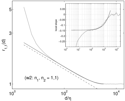
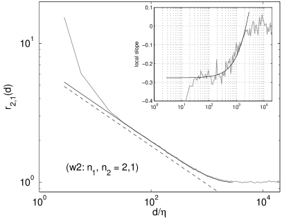
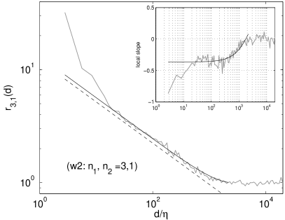
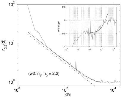
Figure 4: Best fits of expression (11) to two-point correlators extracted from data set w2. Correlation orders are $n_{1},n_{2}=1,1$, $2,1$, $3,1$ and $2,2$. The parameter $L_{\rm casc}$ has been fitted such that it is the same for all orders of two-point correlators as well as two-point cumulants, with the latter illustrated in Fig. 5. The inset figures illustrate the local slope. For comparison, power-law fits with the extracted scaling exponents listed in Tab. II are shown as the shifted dashed straight lines.

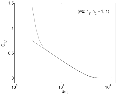
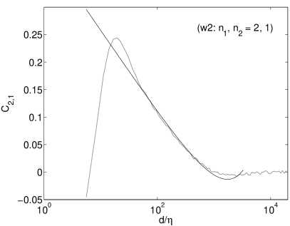
Figure 5: Best fits of expressions (18) to two-point cumulants extracted from data set w2. Correlation orders are $n_{1},n_{2}=1,1$ and $2,1$. The parameter $L_{\rm casc}$ has been fitted such that it is the same for all the orders of two-point cumulants as well as two-point correlators, with the latter illustrated in Fig. 4.

The expressions (11) and (18) come with parameters $L_{\mathrm{casc}}$, $\tau_{n_{1},n_{2}}$, $a_{n_{1},n_{2}}$, $c_{n}$ and $\langle\ln^{n}\Pi\rangle_{c}$. The parameter $L_{\mathrm{casc}}$ depends on neither the order $n_{1},n_{2}$ nor the choice of the two-point statistics, i.e., whether we use the correlator or the cumulant. The fits of (11) and (18) to their counterparts from experimental records have to respect this independence. In addition to the common parameter $L_{\mathrm{casc}}$, the fit of each order has two more parameters: these are $\tau_{n_{1},n_{2}}$, $a_{n_{1},n_{2}}$ for the two-point correlator and $c_{n}$, $\langle\ln^{n}\Pi\rangle_{c}$ for the two-point cumulant. We demonstrate the quality of fits by choosing the data record w2. For this data set, two-point correlators with orders from $n_{1},n_{2}=1,1$ to $2,2$ are illustrated in Fig. 4, while the two-point cumulants with orders $n_{1},n_{2}=1,1$ and $2,1$ are illustrated in Fig. 5. Except for very small two-point distances $\eta\leq d\leq 20{-}30\eta$, where, as already noted, the surrogacy effect of the energy dissipation corrupts the experimental two-point statistics CLE03 , the agreement between the experimental two-point correlators and cumulants and the best-fit expressions (11) and (18) is remarkable. Table II lists the best-fit parameters $L_{\mathrm{casc}}$, $\tau_{n}$ and $c_{n}$. Note that, due to (8) and $\tau_{1}=0$, the scaling exponents $\tau_{n_{1},n_{2}}$ have been converted into $\tau_{2}=\tau_{1,1}$, $\tau_{3}=\tau_{2,1}+\tau_{2}$ and $\tau_{4}=\tau_{3,1}+\tau_{3}=\tau_{2,2}+2\tau_{2}$. For w2 the two values $\tau_{4}=0.79$ and $0.77$, the first value extracted from $r_{3,1}(d)$ and the second from $r_{2,2}(d)$, are consistent with each other, although the statistical convergence of the two two-point correlators of order $n_{1}+n_{2}=4$ is already beyond the limit of acceptability. For the record w3 a similar statement can be made, but the other records w1 and a are definitely confined to $n_{1}+n_{2}\leq 3$. Their best-fit parameters $L_{\mathrm{casc}}$, $\tau_{n}$ and $c_{n}$ are also listed in Table II.

The cumulant $c_{1}$ cannot be directly extracted from two-point cumulants. However, an indirect extraction is possible via the relations (23) and (24). Using the numerical values of $c_{2}$ and $c_{3}$ determined already, the truncated multifractal sum rule (23) leads to the $c_{1}$ values listed in the second-last column of Table 2. Input for the replica-trick formula (24) are the scaling exponents $\tau_{1}$, $\tau_{2}$ and $\tau_{3}$ determined already. The application of a cubic spline for the extrapolation results in the last column of Table 2. If a linear spline is used instead, the resulting $c_{1}$ values of the records w1, w2, w3 shift closer to the values of the second-last column, but would do worse for the record a. For an order-of-magnitude estimate, however, it is safe to say that $c_{1}\approx 0.05$ for the records w1, w2, w3 and $c_{1}\approx 0.07$ for the record a.

This comparison of the RMCP theory with data demonstrates that the parameter $L_{\rm casc}$ is a meaningful quantity and deserves some fundamental consideration. For two-point distances $20{-}30\eta\leq d\leq L_{\rm casc}$, the fitted expressions (11) and (18) are in good qualitative agreement with their experimental counterparts. At $d=L_{\rm casc}$ all two-point correlations decorrelate and become identical to their asymptotic values corresponding to $d\to\infty$; $L_{\rm casc}>L$ is somewhat larger than the operationally defined integral length $L$ of Table I, which is calculated as the correlation length of the velocity autocorrelation function. The physical interpretation of the extracted parameter $L_{\rm casc}$ is that of a turbulent cascade length which, according to Fig. 2, describes the spatial extension of a hierarchical RMCP domain.

The finite-size scaling $f_{n_{1},n_{2}}(d/L_{\rm casc})$ of two-point correlators, predicted by RMCP, now allows for an unambiguous derivation of scaling exponents, even for fully developed turbulent flows with a moderate Reynolds number. Consequently, as a closer inspection of Table II shows, reliable statements that the intermittency exponent $\tau_{2}$ might show a weak dependence on the Reynolds number appear to be within reach. Of course, to make this statement solid, the analysis of many more records is needed; this effort will be reported in CLE03a .

V Parametric estimation of the RMCP generator

If the scaling exponents $\tau_{n}$, or the cumulants $c_{n}$, exist and are known for all orders $1\leq n<\infty$, the binary RMCP generator could in principle be reconstructed via the inverse transform of (21). Unfortunately, as we have seen in the previous section, reliable information is limited to the lowest orders. Hence, the best we can do is to use sophisticated parametric estimates. Section V.A lists some of the most popular parametrizations and compares their performance with the results listed in Table II. Section V.B introduces the so-called log-normal inverse Gaussian distribution BAR98 ; BAR01 , which represents a broader and more flexible parametrization class, with the purpose of finding a suitable approximation to the true cascade generator.

V.1 Dictionary of prototype cascade generators

Here we list a number of popular generators $p(q)$ for binary random multiplicative cascade processes. They all have the property that the expectation value $\langle q\rangle=1$.

The log-normal distribution

$$p_{\rm lognormal}(q)=\frac{1}{\sqrt{2\pi}\sigma q}\exp\left[-{1\over 2\sigma^{2}}\left(\ln q+\frac{\sigma^{2}}{2}\right)^{2}\right]\;$$ (26)

is classic OBU62 ; KOL62 . Its log-stable generalization has also been considered KID91 ; SCH92 , but does not qualify for our purposes, since the cumulants $c_{n}$ do not exist for this distribution beyond some order. For comparison, we will also employ the rescaled gamma distribution

$$p_{\rm gamma}(q)={\gamma^{\gamma}\over\Gamma(\gamma)}q^{\gamma-1}e^{-\gamma q}$$ (27)

and the asymmetric beta distribution JOU00

$$p_{\rm beta}(q)=\frac{\Gamma(8\beta)}{\Gamma(\beta)\Gamma(7\beta)}\;8^{1-8\beta}q^{\beta-1}(8-q)^{7\beta-1}\;.$$ (28)

The bimodal distribution

$$p_{\rm alpha}(q)={\alpha_{2}\over{\alpha_{1}+\alpha_{2}}}\delta\left(q-(1-\alpha_{1})\right)+{\alpha_{1}\over{\alpha_{1}+\alpha_{2}}}\delta\left(q-(1+\alpha_{2})\right)\;,$$ (29)

although discrete, has also been used extensively SCH85 ; MEN87 . Another popular discrete representative is the log-Poisson distribution

$$p_{\rm logPoisson}(q)=\sum_{k=0}^{\infty}\frac{2^{-\nu_{1}}(\nu_{1}\ln{2})^{k}}{k!}\delta\left(q-2^{\nu_{1}(1-\nu_{2})}\nu_{2}^{k}\right)\;,$$ (30)

which was originally derived with $\nu_{1}=2$ and $\nu_{2}=2/3$ from some plausible reasoning on the structure of the most singular objects in fully developed turbulent flows SHE94 ; DUB94 ; SHE95 .

For all parametrizations (26)–(30) it is straightforward to determine analytic expressions for the scaling exponents and cumulants via (20)–(22). The free parameter of the one-parametric distributions (26)–(28) is then fixed to reproduce the observed intermittency exponent $\tau_{2}$, listed in Table II. The two-parametric distributions (29) and (30) need also conform to $\tau_{3}$ in addition to $\tau_{2}$. No further freedom is left for the scaling exponents of higher order and cumulants of all orders. Table III summarizes their predicted values.

It is difficult to rate the prototype cascade generators because of ambiguity inherent in the data. Within the one-parametric distributions (26)-(28) the log-normal distribution performs better: for all the records, the predicted values for $c_{1}$ and $c_{2}$ are close to the observed cumulants. However, the log-normal distribution without skewness is unable to reproduce the observed positive values for $c_{3}$ and for the record w2 it also overestimates the scaling exponent $\tau_{4}$. Furthermore, the difficulties of the log-normal distribution for high-order moments is now well known FRI95 . Compared to the log-normal distribution, the rescaled gamma distribution and the asymmetric beta distribution have the tendency to overestimate the first two cumulants. Furthermore, $c_{3}$ is predicted with an opposite sign. Rather surprisingly, the simple two-parametric bimodal distribution (29) shows the closest agreement for all records. The scaling exponent $\tau_{4}$, if observed, as well as the cumulants $c_{1}$ and $c_{2}$ almost match their observed counterparts. Moreover, $c_{3}$ comes with the correct sign, although it is about a factor $2$ too low for the records w1, w2, w3 and roughly a factor $2$ too large for the atmospheric boundary layer record. Like the distributions (27) and (28), the two-parametric log-Poisson distribution overestimates the second cumulant $c_{2}$ and, except for record w3, predicts $c_{3}$ with the wrong sign. It is interesting to note that the parameter-free log-Poisson distribution SHE94 with $\nu_{1}=2$ and $\nu_{2}=2/3$ matches well the scaling exponents $\tau_{3}$ and $\tau_{4}$ of record a with the largest Reynolds number, but disagrees with all cumulants.

V.2 Log-normal inverse Gaussian distribution

A broader and more flexible parametrization class is the so-called normal inverse Gaussian distribution BAR98 ; BAR01

$$p(x;\alpha,\beta,\mu,\delta)=a(\alpha,\beta,\mu,\delta)\,s\!\left(\frac{x-\mu}{\delta}\right)^{-1}K_{1}\left\{\delta\alpha\,s\!\left(\frac{x-\mu}{\delta}\right)\right\}e^{\beta x}\;,$$ (31)

with $s(x)=\sqrt{(1+x^{2})}$, $a(\alpha,\beta,\mu,\delta)=\pi^{-1}\alpha\exp(\delta\sqrt{\alpha^{2}-\beta^{2}}-\beta\mu)$ and $-\infty{<}x{<}\infty$. $K_{1}$ is the modified Bessel function of the third kind and index 1. The domain of variation of the four parameters is given by $\mu\in\mathbf{R}$, $\delta\in\mathbf{R}_{+}$ and $0\leq|\beta|<\alpha$. The distribution is denoted by $\mathrm{NIG}(\alpha,\beta,\mu,\delta)$, and its cumulant generating function $\mathrm{Q}(\lambda;\alpha,\beta,\mu,\delta)=\ln\langle e^{\lambda x}\rangle$ has the simple form

$$\mathrm{Q}(\lambda;\alpha,\beta,\mu,\delta)=\delta\left(\sqrt{\alpha^{2}-\beta^{2}}-\sqrt{\alpha^{2}-(\beta+\lambda)^{2}}\right)+\mu\lambda\;.$$ (32)

If $x_{1},\ldots,x_{m}$ are independent normal inverse Gaussian random variables with common parameters $\alpha$ and $\beta$ but individual location-scale parameters $\mu_{i}$ and $\delta_{i}$ $(i=1,\ldots,m)$, then $x_{+}=x_{1}+\ldots+x_{m}$ is again distributed according to a normal inverse Gaussian law with parameters $\alpha$, $\beta$, $\mu_{+}$ and $\delta_{+}$. Furthermore, we note that the $\mathrm{NIG}$ distribution (31) has semi-stretched tails

$$p(x;\alpha,\beta,\mu,\delta)\sim\left|x\right|^{-3/2}\exp\left(-\alpha\left|x\right|+\beta x\right)$$ (33)

as $x\rightarrow\pm\infty$. This result follows from the asymptotic relation $K_{\nu}(x{\rightarrow}\infty)\sim\sqrt{\pi/2}x^{-1/2}e^{-x}$.

For our purposes we assume the random multiplicative weight to be distributed according to

$$\ln q\sim\mathrm{NIG}(\alpha,\beta,\delta,\mu)\;,$$ (34)

which turns normal inverse Gaussian statistics into log-normal inverse Gaussian statistics. With (20), (22) and (32), the scaling exponents and cumulants yield

$$\tau_{n}\ln{2}=\mathrm{Q}(n;\alpha,\beta,\mu,\delta)$$ (35)

and

$$c_{1}=\mu+\frac{\delta\rho}{\sqrt{1-\rho^{2}}}\;,\quad c_{2}=\frac{\delta}{\alpha(1-\rho^{2})^{3/2}}\;,\quad c_{3}=\frac{3\delta\rho}{\alpha^{2}(1-\rho^{2})^{5/2}}\;,\quad\ldots\;,$$ (36)

where $\rho=\beta/\alpha$.

For each of the records w1, w2, w3 and a, the four NIG parameters $\alpha$, $\beta$, $\delta$ and $\mu$ are determined so as to reproduce $\tau_{1}=0$ and the observed values for $\tau_{2}$, $\tau_{3}$ and $c_{2}$ listed in Table 2. Since the respective expressions (35) and (36) are nonlinear, real solutions for the parameters are not guaranteed. Where complex-valued solutions resulted in the first attempt, which occurred for w2, w3 and a, the values for $c_{2}$, $\tau_{3}$ and $\tau_{2}$ are relaxed, in this order and to some small extent, until real-valued parameter solutions are obtained. The outcome is listed in Table 4. The results are very close to the log-normal values listed in 3. The log-normal inverse Gaussian distribution has the tendency to overestimate the fourth-order scaling exponent $\tau_{4}$. The magnitude of the third cumulant $c_{3}$ is strongly underestimated, so that its predicted sign shows only random scatter. Figure 6 compares the extracted log-normal inverse Gaussian distributions of Table 4 with the extracted log-normal distributions of Table 3. For all four records the extracted distributions are very similar.

As a summary of this section, we reiterate that the bimodal distribution (29) produces the best overall agreement with the observed scaling exponents and cumulants. However, the true cascade generator will not be discrete. From the set of continuous generator representatives tested, the log-normal and log-normal inverse Gaussian distributions perform best and about equally well.

VI Conclusion

Random multiplicative cascade processes are able to describe the observed two-point correlation structure of the surrogate energy dissipation of fully developed turbulent flows beyond simple power-law scaling. Keeping in mind the need for a satisfactory comparison between modelling and experimental data, a useful transformation has been introduced: this transformation converts model-dependent and unobservable ultrametric two-point distances to Euclidean two-point distances, the latter reflecting the horizontally sampled $n$-point statistics of the experimental records. The predictions of RMCP for finite-size scaling of two-point correlation functions are confirmed by experimental data from three (wind tunnel) shear flows and one atmospheric boundary layer; a new physical length scale characterizing the upper end of the inertial range, called here the turbulent cascade length, has been shown to appear naturally. Furthermore, the quantitative classification of the deviations from a rigorous scaling of two-point correlators allows for an unambiguous extraction of multiscaling exponents, even for flows with moderate Reynolds numbers. When complemented with additional information extracted from two-point cumulants of the logarithmic energy dissipation, reliable parametric estimates of the RMCP generator have become feasible.

RMCPs produce a consistent geometrical modelling of the self-similar turbulent energy cascade. This is further supported by recent investigations on the scaling part of three-point statistics SCH03 and previous investigations on scale correlations JOU99 ; JOU00 ; JOU02 ; CLE00 . Thus, the self-similar and RMCP-like cascade process appears to be universal. However, as shown by variations among the four records considered, the strength of the cascade generator appears to depend on the Reynolds number and perhaps also the flow geometry. This needs further clarification by means of a separate and extended effort CLE03a ; needless to say, there is a strong need for the experimentalists to produce clean and longer records with converged statistics.

data set	$R_{\lambda}$	$L/\eta$	$L_{\rm record}/L$	$\lambda/\eta$	$\Delta x/\eta$
w1	$306$	$484$	$102500$	$35$	$1.97$
w2	$493$	$968$	$193500$	$44$	$2.79$
w3	$1045$	$2564$	$77500$	$64$	$2.97$
a	$9000$	$5{\times}10^{4}$	$1000$	$187$	$1.29$

Table 1: Taylor-scale based Reynolds number $R_{\lambda}$, integral length scale $L$ in units of the dissipation scale $\eta$, record length $L_{\rm record}$, Taylor microscale $\lambda$ and resolution scale $\Delta x$ of three wind tunnel (w1, w2, w3) PEA02 and one atmospheric boundary layer (a) DHR00 records.

data set	$L_{\rm casc}/\eta$	$\tau_{2}$	$\tau_{3}$	$\tau_{4}$	$c_{2}$	$c_{3}$	$c_{1}$(23)	$c_{1}$(24)
w1	1873	0.15	0.46	–	0.100	0.042	-0.057	-0.045
w2	3069	0.15	0.42	0.78	0.095	0.045	-0.055	-0.046
w3	7117	0.17	0.52	0.98	0.099	0.060	-0.059	-0.046
a	322500	0.21	0.58	–	0.149	0.015	-0.077	-0.068

Table 2: Parameter values resulting from least-square fits with expressions (11) and (18). $L_{\rm casc}$ has been fixed for each data set. The last two columns represent the estimates (23) and (24) for the cumulant $c_{1}$.

log-normal distribution (26)
data set	$\sigma$	$\tau_{3}$	$\tau_{4}$	$c_{1}$	$c_{2}$	$c_{3}$
w1	0.33	0.46	0.93	-0.054	0.107	0.000
w2	0.32	0.44	0.87	-0.050	0.101	0.000
w3	0.34	0.51	1.03	-0.059	0.119	0.000
a	0.38	0.63	1.26	-0.073	0.145	0.000
gamma distribution (27)
data set	$\gamma$	$\tau_{3}$	$\tau_{4}$	$c_{1}$	$c_{2}$	$c_{3}$
w1	8.84	0.45	0.87	-0.058	0.120	-0.014
w2	9.41	0.42	0.82	-0.054	0.112	-0.013
w3	7.94	0.50	0.96	-0.064	0.134	-0.018
a	6.39	0.60	1.16	-0.080	0.169	-0.029
beta distribution (28)
data set	$\beta$	$\tau_{3}$	$\tau_{4}$	$c_{1}$	$c_{2}$	$c_{3}$
w1	7.61	0.44	0.85	-0.059	0.124	-0.019
w2	8.11	0.42	0.81	-0.055	0.116	-0.017
w3	6.82	0.49	0.94	-0.066	0.139	-0.025
a	5.47	0.60	1.13	-0.083	0.178	-0.040
bimodal distribution (29)
data set	$\alpha_{1}$    =	$\alpha_{2}$	$\tau_{4}$	$c_{1}$	$c_{2}$	$c_{3}$
w1	0.22	0.52	0.88	-0.049	0.092	0.025
w2	0.24	0.44	0.80	-0.049	0.094	0.018
w3	0.21	0.61	1.00	-0.052	0.094	0.033
a	0.31	0.50	1.06	-0.075	0.144	0.026
log-Poisson distribution (30) with $\nu_{1}=2$, $\nu_{2}=2/3$
	$\tau_{2}$	$\tau_{3}$	$\tau_{4}$	$c_{1}$	$c_{2}$	$c_{3}$
	0.22	0.59	1.06	-0.10	0.228	-0.092
log-Poisson distribution (30)
data set	$\nu_{1}$	$\nu_{2}$	$\tau_{4}$	$c_{1}$	$c_{2}$	$c_{3}$
w1	109.84	0.96	0.90	-0.055	0.111	-0.004
w2	13.75	0.90	0.82	-0.054	0.112	-0.012
w3	1548.7	1.01	1.03	-0.059	0.117	0.001
a	4.61	0.79	1.09	-0.085	0.184	-0.044

Table 3: Fitted parameters for a few prototype cascade generators and their predicted values for the remaining scaling exponents $\tau_{n}$ and cumulants $c_{n}$.

log-normal inverse Gaussian distribution (34)
data set	$\alpha$	$\beta$	$\delta$	$\mu$	$\tau_{2}$	$\tau_{3}$	$\tau_{4}$	$c_{1}$	$c_{2}$	$c_{3}$
w1	10.98	0.94	1.09	-0.14	0.15	0.46	0.95	-0.051	0.100	0.002
w2	17.28	-5.46	1.56	0.47	0.15	0.43	0.85	-0.052	0.106	-0.006
w3	27.26	17.80	1.17	-1.06	0.16	0.52	1.11	-0.052	0.099	0.012
a	6.99	-2.44	0.92	0.27	0.20	0.60	1.19	-0.076	0.160	-0.027

Table 4: Fitted parameters of the log-normal inverse Gaussian cascade generator and their predicted values for the scaling exponents $\tau_{n}$ and cumulants $c_{n}$.

Figure 2: A chain of hierarchical RMCP domains of equal cascade length $L_{\rm casc}$ is employed to convert the ultrametric two-point statistics into an Euclidean one.

Figure 6: Comparison of the extracted log-normal distribution (26) (solid) and log-normal inverse Gaussian distribution (34) (dashed) for the records w1, w2, w3 and a. Respective parameter values have been taken from Tables 3 and 4.