Classical elementary particles, spin,
zitterbewegung and all that

Abstract After a revision of the main features of the structure of the Dirac electron a plausible definition of elementary particle is stated. It is shown that this definition leads in the classical case to a picture which produces a very clear correspondence between the classical and quantum mechanical features of the electron. It is analyzed how the classical spin structure and zitterbewegung are related to the classical variables that define the kinematical state of the particle.

1 Introduction

The very concept of elementary particle seems to be not sufficiently well stated in undergraduate physics books. In most cases they are mentioned as the bricks with which matter can be built. But, if they are so simple objects it is important to establish the theoretical difference between them and other small objects which are not considered as elementary. One of the goals of this work is to introduce some simple ideas which shed light about a theoretical concept of elementary particle and how these ideas lead to their classical and quantum mechanical description.

We know that matter is formed by smaller and smaller units which can be divided again and again into smaller pieces. This process can be continued until we hypothetically reach what the Greeks called an atom, the indivisible unit of matter. Today we call this last division of matter an elementary particle. Elementary particles should be thus the building blocks with which all material systems can be formed.

Leptons and quarks are the basic elementary particles in the standard model picture. They all have, as intrinsic properties, mass, spin 1/2, electric charge and several other quantum numbers with some exotic names as baryon and lepton number, isotopic spin, strangeness, beauty and others. Together the intermediate spin 1 bosons, which carry the interactions between them, we have a collection of, charged and uncharged, spinning objects. It seems that there are no spinless elementary particles in nature, so that the spin description is crucial for the understanding of the structure of matter. Whether or not these todays considered elementary particles can be subsequently divided is still an open question. But if these final indivisible objects exist, it is possible to state, at least from the theoretical point of view, what are the necessary conditions for a mechanical system to be considered as elementary, to be considered as the ending process of division of matter.

To fix ideas we review in the next section, the description, from the classical and quantum mechanical point of view, of the structure of the electron.

We state in section 3 the concept of elementary particle as a mechanical system without excited states. The description of the state of an elementary particle is reduced to the analysis of the updated consecutive inertial observers which describe the particle in the same state. The remaining sections are devoted to the analysis of the kind of Lagrangian systems the above definition allows to deal with, in particular with the relativistic and non-relativistic point particle and more important, of the spinning systems. We end this work with the classical Lagrangian description of the photon and a final section devoted to general conclusions and some difficulties of the formalism.

2 What is an electron?

The usual attempt to describe classically the spinning electron has been to endow the Newtonian point particle with some spherical shape of small radius, some plausible charge distribution on its surface or in its whole volume, and a final rotation as a rigid body to give account of the spin angular momentum. Nevertheless this rigid body description has led to serious difficulties. One needs to justify how the charge is held together and therefore the additional description of the glue forces is necessary. With a finite radius and a uniform mass distribution the velocity of the outer part of the sphere should exceed the velocity of light to obtain the measured values of the spin.

The failure of this kind of classical models led Barut to quote about the structure of the spinning electron: ‘If a spinning particle is not quite a point particle, nor a solid three dimensional top, what can it be? What is the structure which can appear under probing with electromagnetic fields as a point charge, yet as far as spin and wave properties are concerned exhibits a size of the order of the Compton wavelength?’ [1].

Nevertheless, for the description of the electron what we have is the quantum mechanical Dirac’s analysis. Dirac equation has as many negative energy solutions as positive energy ones, and one of the success of this formalism is the interpretation of the negative energy solutions as representing positive energy solutions of a particle of the same intrinsic attributes mass and spin 1/2 but opposite electric charge. Every charged spin 1/2 particle has an antiparticle.

If point $r$ is the position vector on which Dirac’s spinor $\psi(t,{\mbox{\boldmath$r$}})$ is defined, then, when analyzing the velocity of point $r$, Dirac finds that: [2]

1. The velocity ${\mbox{\boldmath$v$}}=i/\hbar[H,{\mbox{\boldmath$r$}}]=c\mbox{\boldmath$\alpha$}$, is expressed in terms of $\alpha$ matrices, which have eigenvalues $\pm 1$, and the velocity of light $c$, and writes:
   ‘$\ldots$ a measurement of a component of the velocity of a free electron is certain to lead to the result $\pm c$. This conclusion is easily seen to hold also when there is a field present.’

2. One of the puzzling features of this description is that the linear momentum $p$ does not have the direction of the velocity $v$ of point $r$, but it is related to some average value of it: ${\ldots}$ ‘the $x_{1}$ component of the velocity, $c\alpha_{1}$, consists of two parts, a constant part $c^{2}p_{1}H^{-1}$, connected with the momentum by the classical relativistic formula, and an oscillatory part, whose frequency is at least $2mc^{2}/h$, ${\ldots}$’.
   It seems that point $r$ does not represent the center of mass position of the electron.

3. The position $r$ oscillates very fast in a small region of order of Compton’s wavelength:
   ‘The oscillatory part of $x_{1}$ is small, ${\ldots}$ , which is of order of magnitude $\hbar/mc$, ${\ldots}$’.
   This oscillatory motion of point $r$ was defined by Schrödinger as the zitterbewegung or quivering or trembling motion of the electron.

4. In his Nobel dissertation lecture he insists on this peculiar feature of the quivering motion at the speed of light of the electron: [3]
   ‘The new variables $\alpha$, which we have to introduce to get a relativistic wave equation linear in $H$, give rise to the spin of the electron. From the general principles of quantum mechanics one can easily deduce that these variables $\alpha$ give the electron a spin angular momentum of half a quantum and a magnetic moment of one Bohr magneton in the reverse direction to the angular momentum. These results are in agreement with experiment. They were, in fact, first obtained from the experimental evidence provided by spectroscopy and afterwards confirmed by the theory.’
   ‘The variables $\alpha$ also give rise to some rather unexpected phenomena concerning the motion of the electron. These have been fully worked out by Schrödinger. It is found that an electron which seems to us to be moving slowly, must actually have a very high frequency oscillatory motion of small amplitude superposed on the regular motion which appears to us. As a result of this oscillatory motion, the velocity of the electron at any time equals the velocity of light. This is a prediction which cannot be directly verified by experiment, since the frequency of the oscillatory motion is so high and its amplitude is so small. But one must believe in this consequence of the theory, since other consequences of the theory which are inseparably bound up with this one, such as the law of scattering of light by an electron, are confirmed by experiment.’
   The electron has thus a regular motion, which can be easily interpreted as the motion of its center of mass, and the oscillatory motion of point $r$ at the velocity of light around the center of mass. The absolute value of the velocity $c$ is not modified by the presence of an external field.

5. The total angular momentum of a free electron ${\mbox{\boldmath$J$}}={\mbox{\boldmath$r$}}\times{\mbox{\boldmath$P$}}+{\mbox{\boldmath$S$}}={\mbox{\boldmath$L$}}+{\mbox{\boldmath$S$}}$, is a constant of the motion, but the orbital part $L$ and the spin $S$ are not separately constants of the motion. The spin $S$ of a free electron satisfies the dynamical equation

   $$\frac{d{\mbox{\boldmath$S$}}}{dt}={\mbox{\boldmath$p$}}\times c{\mbox{\boldmath$\alpha$}}={\mbox{\boldmath$p$}}\times{\mbox{\boldmath$v$}},$$

   so that the spin operator $S$ is only a constant of the motion for the center of mass observer for which ${\mbox{\boldmath$p$}}=0$.

6. In his original 1928 paper [4], when analyzing the interaction of the electron with an external electromagnetic field, after developing the interaction Hamiltonian to first order in the external fields, he obtains two new interaction terms:

   $${e\hbar\over 2m}{\bf\Sigma}\cdot{\mbox{\boldmath$B$}}+{ie\hbar\over 2mc}\mbox{\boldmath$\alpha$}\cdot{\mbox{\boldmath$E$}}=-\mbox{\boldmath$\mu$}\cdot{\mbox{\boldmath$B$}}-{\mbox{\boldmath$d$}}\cdot{\mbox{\boldmath$E$}},$$ (1)

   where Dirac’s electron spin operator is written as

   $${\mbox{\boldmath$S$}}=\frac{\hbar}{2}{\bf\Sigma}=\frac{\hbar}{2}\pmatrix{\mbox{\boldmath$\sigma$}&0\cr 0&\mbox{\boldmath$\sigma$}\cr},$$

   in terms of $\sigma$-Pauli matrices and where $E$ and $B$ are the external electric and magnetic fields, respectively. He says: ‘the electron will therefore behave as though it has a magnetic moment $-(e\hbar/2m)\,{\bf\Sigma}$ and an electric moment $-(ie\hbar/2mc)\,\mbox{\boldmath$\alpha$}$. The magnetic moment is just that assumed in the spinning electron model’. ‘The electric moment, being a pure imaginary, we should not expect to appear in the model. It is doubtful whether the electric moment has any physical meaning.’

The electron, in addition to the electric charge behaves as though it has some electric and magnetic dipole moments. The magnetic dipole term is the right one to give account of the Zeeman effect in atoms. But, what about the electric dipole? In the last Dirac sentence it is difficult to understand why Dirac, who did not reject the negative energy solutions, and therefore its consideration as the antiparticle states, and insisted that the motion of point $r$ is at the speed of light as an ‘inseparably bound up’ consequence, disliked the existence of this electric dipole which was obtained from his formalism on an equal footing and at the same time as the magnetic dipole term. In his book and in the Noble dissertation he never mentioned again this electric dipole property. But, what happens if the point $r$ represents the position of the center of charge of the electron. By the previous analysis it seems to be a different point than the center of mass. Then this separation implies that for the center of mass observer there is a nonvanishing electric dipole moment. It is oscillating very fast, its average value is probably zero, but it is a physical property that has to be taken into account.

In fact, in quantum electrodynamics, the complete Dirac Hamiltonian contains both terms, perhaps in an involved way because the above expression (1) is a first order expansion in the external fields considered as classical commuting fields. It might happen that this electric dipole does not represent the existence of a particular positive and negative charge distribution for the electron, but rather a separation between the center of mass and center of charge. This interpretation will be obtained later when analyzing the classical spinning models.

3 What is an elementary particle?

The concept of elementary particle rests on the idea that this ultimate indivisible object is a so simple mechanical system that it has no excited states. In a broad sense it is always in a single state which looks different for the different inertial observers, but the difference is only a matter of change of point of view and not a change of its intrinsic properties. It is only a kinematical change.

In the quantum case, once a single inertial observer $O$ describes the state of the electron, the collection of the remaining states described by all other inertial observers completely reproduce the Hilbert space of all states. These states can be obtained from the previous one by the corresponding transformation of the wave function to the new frames. There is no other possible state of the electron which cannot be described by any one of the above states or any linear combination of them. The Hilbert space is the kinematical state space of an elementary particle. This set of states contains only kinematical modifications of any one of them.

This is Wigner’s quantum definition of an elementary particle as a system whose Hilbert space of pure states is an invariant space under the group of space-time transformations. In group theoretical language, an elementary particle is thus a quantum system whose Hilbert space of states carries an irreducible representation of the kinematical group of space-time transformations. [5]

It is clear that Wigner’s irreducibility condition is a necessary condition for a quantum system to be considered as elementary. But, what is the classical equivalent requirement?

Let us assume that a particular inertial observer is describing the classical state of a particle by giving the values of the basic and essential variables which characterize its state. Now the particle, under some external influence, changes some of its variables and therefore it goes into a different state. Then, by assumption, if the particle is elementary it is always possible to select another inertial observer who describes the particle in the same state and with the same values of its variables as the previous observer. This is the idea about what an elementary particle should be from a theoretical viewpoint. Every change in the state of an elementary particle can always be compensated by choosing a new inertial reference frame.

This idea imposes very stringent conditions on what are the classical variables we need to describe the states of an elementary particle. For instance, if the particle has some directional property like spin and the spin orientation changes, the new inertial observer should accommodate its reference frame to describe the spin components as before and therefore its frame looks rotated with respect to the previous one. By following the change of orientation of the updated inertial frames, we are describing the change of orientation of the spin of the particle, and thus the spin dynamics.

At this stage we do not know yet what are the classical variables to describe an elementary particle. But instead of describing the particle let us try to describe the collection of consecutive updated inertial observers who instantaneously describe the elementary particle by the same state. By describing every one of these particular inertial observers we are describing the instantaneous kinematical state of the elementary particle. By describing the instantaneous change of these inertial observers we are describing the dynamical behavior of the particle.

Let us see first how we use to describe every reference inertial frame with respect to each other. This is very deeply related to a restricted relativity principle.

4 The Restricted Relativity Principle

A very fundamental principle is a Restricted (sometimes called Special) relativity principle. By restricted it is meant that the fundamental laws of physics have to be invariant for a restricted set of equivalent observers, called inertial observers. It is also called restricted to distinguish from a General relativity principle in which all observers, accelerated or not, describe nature by the same form invariant laws.

The relationship between the different inertial observers is related to their relative measurement of space-time events, i.e., to how they relate the time and position coordinates of the same and every space-time event. This relationship is defined by a space-time transformation group which is called a kinematical group. Different kinematical groups containing as possible transformations space and time translations, rotations and boosts, are analyzed by Bacry and Levy-Leblond in [6]. Among them we find the Galilei and Poincaré group and also the de Sitter groups. But more general groups, like the conformal group, could be good candidates as kinematical groups. If we restrict ourselves to the Galilei and Poincaré group we shall obtain only as intrinsic attributes of matter the value of the mass and spin, which are the two group invariant properties. Other quantum numbers have no so clear classical interpretation and are related to the so called ‘internal’ symmetry groups.

Let us consider first the Galilei group. The relationship between two arbitrary inertial observers is:

$$t^{\prime}=t+b,\quad{\mbox{\boldmath$r$}}^{\prime}=R(\mbox{\boldmath$\alpha$}){\mbox{\boldmath$r$}}+{\mbox{\boldmath$v$}}t+{\mbox{\boldmath$d$}}.$$

Observer $O$ measures the coordinates $t$ and $r$ of a particular space-time event while observer $O^{\prime}$ obtains the coordinates $t^{\prime}$ and ${\mbox{\boldmath$r$}}^{\prime}$ for the same event. Then the remaining variables of the above formulae $b$, $d$, $v$ and $R(\mbox{\boldmath$\alpha$})$, which are constant once the two inertial observers are fixed, define the relative relationship between them. Any relative measurement between them of any other physical property of a system will depend on these constants. Let us see their meaning.

Suppose observer $O$ measures the emission of a burst of light from the origin of its Cartesian frame ${\mbox{\boldmath$r$}}=0$ when its clock shows $t=0$. This event takes place for $O^{\prime}$ at time $t^{\prime}=b$ and at the point ${\mbox{\boldmath$r$}}^{\prime}={\mbox{\boldmath$d$}}$. If at instant $dt$ observer $O$ measures another light burst form its origin, it takes the values $t^{\prime}+dt^{\prime}=dt+b$ and ${\mbox{\boldmath$r$}}^{\prime}+d{\mbox{\boldmath$r$}}^{\prime}={\mbox{\boldmath$v$}}dt+{\mbox{\boldmath$d$}}$, i.e., after a time $dt^{\prime}=dt$ and displaced $d{\mbox{\boldmath$r$}}^{\prime}={\mbox{\boldmath$v$}}dt$ with respect to the previous event. Therefore the origin of $O$ is moving with a velocity $d{\mbox{\boldmath$r$}}^{\prime}/dt^{\prime}={\mbox{\boldmath$v$}}$ as measured by $O^{\prime}$. Finally $R(\mbox{\boldmath$\alpha$})$ represents how the Cartesian unit vectors of $O$ are represented in $O^{\prime}$ frame if they were at relative rest.

Then $O^{\prime}$ describes observer $O$ by giving at its time $b$ the position of the origin of $O$ frame at $d$, moving with velocity $v$ and with three unit vectors linked to it and oriented according to $R(\mbox{\boldmath$\alpha$})$. We say that $O^{\prime}$ specifies any other inertial observer by some fixed values of the time, the position of a point, velocity of that point and orientation around that point. That’s all.

5 Classical Elementary Particles

Let us think now that we consider ourselves identified with the observer $O^{\prime}$ and we are measuring the evolution of an elementary particle in terms of some arbitrary evolution parameter $\tau$, which can be our own time or any other monotonic function of it. Now let us focus our attention to some particular inertial observer. It can be, for instance, an inertial observer very close to the particle or an inertial observer located in some specific part of the system. Then, at instant $\tau$, we fix this particular inertial observer by giving the ten variables $(t(\tau),{\mbox{\boldmath$r$}}(\tau),{\mbox{\boldmath$v$}}(\tau),\mbox{\boldmath$\alpha$}(\tau))$, with the same meaning respectively as before, although we have partially changed the notation. The time translation parameter $b$ has been replaced by the time observable $t(\tau)$ and the position of the origin $d$ by ${\mbox{\boldmath$r$}}(\tau)$. By $\mbox{\boldmath$\alpha$}(\tau)$ we mean the three parameters which can be used to describe the orientation of any frame. They can be Euler’s angles or any other parametrization of the rotation group. In any case we give the values of a time $t$, the position of a point $r$, the velocity of this point $v$ and the orientation around this point $\alpha$ or the matrix of the three unit vectors $R(\mbox{\boldmath$\alpha$})$.

Now at instant $\tau+d\tau$ the particle has changed, so that the new selected inertial observer who sees the particle in the same state as the previous inertial observer, is described by the new variables $(t(\tau+d\tau),{\mbox{\boldmath$r$}}(\tau+d\tau),{\mbox{\boldmath$v$}}(\tau+d\tau),\mbox{\boldmath$\alpha$}(\tau+d\tau))$. The group structure of the Galilei group implies that the relationship between these two inertial observers is given by an infinitesimal element of the Galilei group $\delta g$ of parameters $(dt,d{\mbox{\boldmath$r$}},d{\mbox{\boldmath$v$}},d\mbox{\boldmath$\alpha$})$, so that the change of the action of the system between instants $\tau$ and $\tau+d\tau$ is given to first order in terms of these variations by

$$Ld\tau=Tdt+{\mbox{\boldmath$R$}}\cdot d{\mbox{\boldmath$r$}}+{\mbox{\boldmath$V$}}\cdot d{\mbox{\boldmath$v$}}+{\mbox{\boldmath$A$}}\cdot d\mbox{\boldmath$\alpha$}=(T\dot{t}+{\mbox{\boldmath$R$}}\cdot\dot{\mbox{\boldmath$r$}}+{\mbox{\boldmath$V$}}\cdot\dot{\mbox{\boldmath$v$}}+{\mbox{\boldmath$A$}}\cdot\dot{\mbox{\boldmath$\alpha$}})d\tau,$$

where the overdot means derivation with respect to the evolution parameter $\tau$. We do not know yet the functions $T$, $R$, $V$ and $A$, but what is clear is that the most general Lagrangian which describes this system must be a function of the kinematical variables $(t,{\mbox{\boldmath$r$}},{\mbox{\boldmath$v$}},\mbox{\boldmath$\alpha$})$ and their first order $\tau$ derivatives.

The evolution of the system in the interval $[\tau_{1},\tau_{2}]$ is described, once the Lagrangian is known, by giving these kinematical variables $(t,{\mbox{\boldmath$r$}},{\mbox{\boldmath$v$}},\mbox{\boldmath$\alpha$})\equiv x(\tau_{1})$ at instant $\tau_{1}$ and the values of the same variables at the final instant $\tau_{2}$, $x(\tau_{2})$. The variational principle implies that the path followed by the system between these fixed end points $x(\tau_{1})$ and $x(\tau_{2})$, is the one which produces a minimum for the action of the system. The kinematical or evolution space of this Lagrangian system is just the manifold spanned by these initial (or final) points. But, because any infinitesimal change is produced by an infinitesimal element of the Galilei group $\delta g$, the composition of all these consecutive infinitesimal group elements will produce in general a finite group element $g$ such that $x(\tau_{2})=gx(\tau_{1})$. The manifold spanned by these variables has the property that given any two points there exists at least a group element $g$ that relates them. In group theory it is said that the group acts transitively on this manifold or that the manifold is a homogeneous space of the group.

We conclude that the kinematical space of a classical elementary particle must necessarily be a homogeneous space of the kinematical group. This is the classical requirement equivalent to the irreducibility condition of the quantum case to define a classical elementary particle.

Although we started this analysis with the Galilei group we see that the parametrization of the Poincaré group leads to the same kind of ten variables $(t,{\mbox{\boldmath$r$}},{\mbox{\boldmath$v$}},\mbox{\boldmath$\alpha$})$, and with the same geometrical meaning as before, to characterize the relative description of every inertial observer. This implies that, even in the relativistic case, the most general Lagrangian of a classical elementary particle can be written as before as

$$L=T\dot{t}+{\mbox{\boldmath$R$}}\cdot\dot{\mbox{\boldmath$r$}}+{\mbox{\boldmath$V$}}\cdot\dot{\mbox{\boldmath$v$}}+{\mbox{\boldmath$A$}}\cdot\dot{\mbox{\boldmath$\alpha$}}.$$ (2)

As a matter of fact we see that the Newtonian point particle is a classical elementary particle, according to this definition. The kinematical space is spanned by $t$ and $r$, which is a homogeneous space of the Galilei group. Because the free motion is at a constant speed and the particle has no orientation properties, it is not necessary to modify neither the velocity $v$ nor the orientation $\alpha$ of the successive inertial observers, so that the variation of the action is written as

$$Ld\tau=(T\dot{t}+{\mbox{\boldmath$R$}}\cdot\dot{\mbox{\boldmath$r$}})d\tau,$$

and the most general free Lagrangian for a point particle is a function of $t$, $r$ and their first order $\tau-$derivatives. Variables $t$ and $r$ are interpreted as the time and position observable of the particle, respectively, and in a time evolution description the Lagrangian will be also a function of the velocity $d{\mbox{\boldmath$r$}}/dt$. The above expansion suggests that the Lagrangian can be written as

$$L=T\dot{t}+{\mbox{\boldmath$R$}}\cdot\dot{\mbox{\boldmath$r$}}.$$ (3)

If the Lagrangian of any Lagrangian system is written in terms of the kinematical variables, i.e., in terms of the end point variables $x_{i}$ of the variational formalism, instead of the independent degrees of freedom, then the Lagrangian is a homogeneous function of first degree of the $\tau-$derivatives of the kinematical variables $\dot{x}_{i}$. Therefore, Euler’s theorem on homogenous functions of first degree in $\dot{x}_{i}$ imply

$$L(x,\dot{x})=\frac{\partial L}{\partial\dot{x}_{i}}\,\dot{x}_{i},$$

with the usual addition convention on repeated indexes. This homogeneity property can be seen for instance in [7] in which a detailed analysis of this property, even for generalized Lagrangians depending on higher order derivatives, is worked out.

Then the above expansion (3) is just this homogeneity condition and thus

$$T=\frac{\partial L}{\partial\dot{t}},\quad{\mbox{\boldmath$R$}}=\frac{\partial L}{\partial\dot{\mbox{\boldmath$r$}}}.$$

In the $\tau-$evolution description we see in the non-relativistic case

$$Ldt=L\dot{t}\,d\tau=\frac{m}{2}\left(\frac{d{\mbox{\boldmath$r$}}}{dt}\right)^{2}\dot{t}\,d\tau=\frac{m}{2}\frac{{\dot{\mbox{\boldmath$r$}}}^{2}}{\dot{t}}d\tau\equiv\widehat{L}(x,\dot{x})d\tau$$

i.e., $\widehat{L}(x,\dot{x})=m{\dot{\mbox{\boldmath$r$}}}^{2}/2\dot{t}$, a homogeneous function of first degree in terms of $\dot{t}$ and $\dot{\mbox{\boldmath$r$}}$.

Similarly, in the relativistic case, the space-time manifold is also a homogeneous space of the Poincaré group. We also get for the point particle Lagrangian a homogenous function of first degree in terms of the derivatives of the kinematical variables

$$\widehat{L}(x,\dot{x})=-mc\sqrt{c^{2}{\dot{t}}^{2}-{\dot{\mbox{\boldmath$r$}}}^{2}},$$

since it is the square root of a second order polynomial in terms of the $\dot{x}$.

When compared the point particle Lagrangian (3) with the most general Lagrangian (2), we see that new possible terms depending on $\dot{\mbox{\boldmath$v$}}$ and $\dot{\mbox{\boldmath$\alpha$}}$ should appear. It is from the dependence on these new variables that the spin structure of the particle and the zitterbewegung of point $r$ will emerge.

6 Spinning Elementary Particles

We propose the name of kinematical theory of elementary particles for this formalism because the kinematical space of the system is basically related, as a homogeneous space, to the kinematical group of space-time transformations. Not only the kinematical group defines the space-time symmetries of the system, but it also supplies the classical variables which characterize the description of a classical elementary particle. It is the kinematical group of space-time transformations which defines the structure of the Lagrangian of an elementary particle. We remit the reader to the published research works on this subject for the different technical points and limit ourselves to outline the main features of the formalism [8].

One technical thing is that the invariance of the dynamical equations under the kinematical group of transformations does not mean that the Lagrangian has to be invariant. The invariance or not of the Lagrangian is related to the group structure [9]. In the non-relativistic case the Lagrangian transforms under the Galilei group up to a total $\tau-$derivative, while it is invariant under the Poincaré group, provided the kinematical variables that define the mechanical system span a homogeneous space of the group. If these kinematical variables do not span a homogeneous space the Lagrangians are no longer invariant, as it happens for compound systems.

The most general particle has thus ten kinematical variables $x\equiv(t,{\mbox{\boldmath$r$}},{\mbox{\boldmath$v$}},\mbox{\boldmath$\alpha$})$, which correspond to a mechanical system of six degrees of freedom. Three represent the position of a point $r$ and the other three $\alpha$, its orientation in space like a rigid body. But, since the Lagrangian also depends on $\dot{x}$ it will depend on the derivative of $v$, and thus the second derivative of $r$ and on the first derivative of $\alpha$. Since the most general Lagrangian for an elementary particle depends on the acceleration of point $r$, the dynamical equations of this point will be of fourth order. Analysis and description of the relativistic and non-relativistic fourth order differential equations to describe the spinning electron are obtained in [10].

Instead of the dependence of the Lagrangian on the derivative of the orientation $\dot{\mbox{\boldmath$\alpha$}}$ is better to use the angular velocity $\omega$, which is a linear function of $\dot{\mbox{\boldmath$\alpha$}}$, and the part of the Lagrangian ${\mbox{\boldmath$A$}}\cdot\dot{\mbox{\boldmath$\alpha$}}$ is replaced by ${\mbox{\boldmath$W$}}\cdot{\mbox{\boldmath$\omega$}}$, with ${\mbox{\boldmath$W$}}=\partial L/\partial{\mbox{\boldmath$\omega$}}$. In fact

$${\mbox{\boldmath$A$}}\cdot\dot{\mbox{\boldmath$\alpha$}}\equiv\frac{\partial L}{\partial\dot{\alpha}_{i}}\dot{\alpha}_{i}=\frac{\partial L}{\partial\omega_{j}}\frac{\partial\omega_{j}}{\partial\dot{\alpha}_{i}}\dot{\alpha}_{i}=\frac{\partial L}{\partial\omega_{j}}\omega_{j}\equiv{\mbox{\boldmath$W$}}\cdot{\mbox{\boldmath$\omega$}}.$$

The most general structure of the Lagrangian, in a relativistic and non-relativistic formalism, is thus

$$L=T\dot{t}+{\mbox{\boldmath$R$}}\cdot\dot{\mbox{\boldmath$r$}}+{\mbox{\boldmath$V$}}\cdot\dot{\mbox{\boldmath$v$}}+{\mbox{\boldmath$W$}}\cdot{\mbox{\boldmath$\omega$}},$$ (4)

where $T=\partial L/\partial\dot{t}$, ${\mbox{\boldmath$R$}}=\partial L/\partial\dot{\mbox{\boldmath$r$}}$, ${\mbox{\boldmath$V$}}=\partial L/\partial\dot{\mbox{\boldmath$v$}}$, and ${\mbox{\boldmath$W$}}=\partial L/\partial{\mbox{\boldmath$\omega$}}$, as before, to be determined once the Lagrangian is given. In general, since we postulate translation and rotation invariance, the Lagrangian will be independent of $t$, $r$ and $\alpha$.

Although we have not formulated yet any particular Lagrangian it is possible to give some general features of the different systems in terms of the general expression (4) and of these defined momenta. Noether’s theorem, under the Galilei group transformations, gives rise to the ten following constants of the motion: [7]

Under translations, the energy and linear momentum, respectively

$$H=-T-{\mbox{\boldmath$v$}}\cdot\frac{d{\mbox{\boldmath$V$}}}{dt},\quad{\mbox{\boldmath$P$}}={\mbox{\boldmath$R$}}-\frac{d{\mbox{\boldmath$V$}}}{dt},$$ (5)

under boosts the kinematical momentum

$${\mbox{\boldmath$K$}}=m{\mbox{\boldmath$r$}}-{\mbox{\boldmath$P$}}t-{\mbox{\boldmath$V$}},$$ (6)

and finally under rotations the angular momentum

$${\mbox{\boldmath$J$}}={\mbox{\boldmath$r$}}\times{\mbox{\boldmath$P$}}+{\mbox{\boldmath$v$}}\times{\mbox{\boldmath$V$}}+{\mbox{\boldmath$W$}}={\mbox{\boldmath$L$}}+{\mbox{\boldmath$S$}}.$$ (7)

The time derivative of the constant $K$ leads to

$${\mbox{\boldmath$P$}}=m{\mbox{\boldmath$v$}}-\frac{d{\mbox{\boldmath$V$}}}{dt},$$

and compared with (5) we get that ${\mbox{\boldmath$R$}}=m{\mbox{\boldmath$v$}}$, and the linear momentum of the system has not the direction of the velocity of the point $r$, provided the Lagrangian depends on the acceleration, and therefore the term $V$ is nonvanishing. Point $r$ does not represent the center of mass position of the particle. In fact if we define the position of a point $q$ by

$${\mbox{\boldmath$q$}}={\mbox{\boldmath$r$}}-{\mbox{\boldmath$V$}}/m\equiv{\mbox{\boldmath$r$}}-{\mbox{\boldmath$k$}},$$

then the kinematical momentum can be written as ${\mbox{\boldmath$K$}}=m{\mbox{\boldmath$q$}}-{\mbox{\boldmath$P$}}t$, and its time derivative leads to ${\mbox{\boldmath$P$}}=md{\mbox{\boldmath$q$}}/dt$. Point $q$, which is a different point than $r$ whenever $V$ is different from zero, represents the position of the centre of mass of the particle. Vector ${\mbox{\boldmath$k$}}={\mbox{\boldmath$V$}}/m$, represents the relative position of point $r$ with respect to the center of mass $q$.

The angular momentum (7) contains two parts: One, ${\mbox{\boldmath$L$}}={\mbox{\boldmath$r$}}\times{\mbox{\boldmath$P$}}$, which is the orbital angular momentum of the system with respect to the origin, and another ${\mbox{\boldmath$S$}}={\mbox{\boldmath$v$}}\times{\mbox{\boldmath$V$}}+{\mbox{\boldmath$W$}}$, which is translation invariant and can be interpreted as the spin of the system. The orbital angular momentum is not a constant of the motion because $P$ is not pointing along the velocity of point $r$. After taking the time derivative of the constant angular momentum we get that the spin of a free particle satisfies the dynamical equation

$$\frac{d{\mbox{\boldmath$S$}}}{dt}={\mbox{\boldmath$P$}}\times{\mbox{\boldmath$v$}},$$ (8)

which is the same dynamical equation satisfied by the Dirac spin operator in the quantum formulation. It is the classical spin observable equivalent to Dirac’s spin operator.

We see that the structure of the spin is twofold. One ${\mbox{\boldmath$W$}}=\partial L/\partial\mbox{\boldmath$\omega$}$, coming from the dependence of the Lagrangian on the angular velocity, like in a rigid body, and we thus expect to be along the angular velocity for a spherical symmetric object, and another ${\mbox{\boldmath$v$}}\times{\mbox{\boldmath$V$}}$, orthogonal to the velocity of point $r$, which can be written in terms of the relative position vector $k$ as

$${\mbox{\boldmath$v$}}\times{\mbox{\boldmath$V$}}=-{\mbox{\boldmath$k$}}\times m{\mbox{\boldmath$v$}}.$$

It looks like an (anti-)orbital part of the momentum $m{\mbox{\boldmath$v$}}$ located at $r$ with respect to the center of mass. The term anti-orbital comes because of the minus sign in front of it.

That point $r$ represents the position of the charge can be seen when we consider the interaction of the system with some external source. The most general interaction Lagrangian will be of the form

$$L_{I}=-\phi\dot{t}+{\mbox{\boldmath$A$}}\cdot\dot{\mbox{\boldmath$r$}},$$

i.e., what is called the minimal coupling, independent of the variables $\dot{\mbox{\boldmath$v$}}$ and $\omega$ because if the system is elementary its spin cannot be modified by the interaction. The presence of terms in $\dot{\mbox{\boldmath$v$}}$ and $\omega$ in the interaction Lagrangian, will produce a modification of the functions $V$ and $W$ which define the spin. If we assume that the external potentials $\phi$ and $A$ are only functions of $t$ and $r$, then the external force is the Lorentz force where the fields are defined at the position $r$ and it is the velocity of point $r$ which enters into the magnetic force term.

7 The Classical Relativistic Spinning Electron

In the relativistic case we have three possible maximal, disjoint, homogeneous spaces of the Poincaré group, spanned by the ten variables $(t,{\mbox{\boldmath$r$}},{\mbox{\boldmath$v$}},\mbox{\boldmath$\alpha$})$, provided $v$ is lesser, greater or equal to $c$. The very important manifold for the description of the classical photon and electron is the one with $v=c$, because it describes a system whose position vector $r$, which is not the center of mass of the system, it is moving at the speed of light. The importance of this manifold is suggested by Dirac’s previous analysis of the electron. In fact, it is the quantization of this system which leads to Dirac equation [11].

The Lagrangian has the same expansion in terms of the derivatives as in (4). For this system there is a small difference in the Noether constants of the motion, with respect to the Galilei case. The expression for $H$, $P$ and $J$ is the same as in (5) and (7). The $K$ momentum is now given by

$${\mbox{\boldmath$K$}}=\frac{1}{c^{2}}H{\mbox{\boldmath$r$}}-{\mbox{\boldmath$P$}}t-\frac{1}{c^{2}}{\mbox{\boldmath$S$}}\times{\mbox{\boldmath$v$}},$$ (9)

with ${\mbox{\boldmath$S$}}={\mbox{\boldmath$v$}}\times{\mbox{\boldmath$V$}}+{\mbox{\boldmath$W$}}$, which satisfies the same dynamical equation as before (8), and is only a constant of the motion in the center of mass frame. The center of mass (or center of energy) of the electron is defined now as:

$${\mbox{\boldmath$q$}}={\mbox{\boldmath$r$}}-\frac{1}{H}{\mbox{\boldmath$S$}}\times{\mbox{\boldmath$v$}},$$

because it leads to ${\mbox{\boldmath$P$}}=(H/c^{2})d{\mbox{\boldmath$q$}}/dt$, by derivation of $K$. Whenever the spin of the system is different from zero the center of mass is a different point than $r$, which, by the same arguments as before, represents the position of the charge.

For the center of mass observer ${\mbox{\boldmath$q$}}=0$, the spin is a constant of the motion, $H=mc^{2}$ and thus

$${\mbox{\boldmath$r$}}=\frac{1}{mc^{2}}{\mbox{\boldmath$S$}}\times{\mbox{\boldmath$v$}},$$ (10)

so that point $r$ is moving in circles, at the speed of light, on a plane orthogonal to the constant vector $S$. Classical mechanics does not restrict the value of the constant spin $S$ which can be any positive real number. Its true value will be uniquely fixed after quantization. The radius of this circle is $R=S/mc$ and the angular velocity of this internal motion or zitterbewegung is $\omega=mc^{2}/S$. By inspection of (10) we see that the relative orientation between the different magnitudes is the one depicted in fig.1, in which we also depict the two parts of the spin ${\mbox{\boldmath$S$}}_{\omega}={\mbox{\boldmath$W$}}$ along the angular velocity $\omega$, and the antiorbital ${\mbox{\boldmath$S$}}_{v}={\mbox{\boldmath$v$}}\times{\mbox{\boldmath$V$}}$, orthogonal to the zitterbewegung plane. The antiparticle corresponds to the time reversed motion, or to consider that $H=-mc^{2}$.

Figure 1: Evolution of point $r$ in the center of mass frame. The body frame, which rotates with angular velocity $\omega$, is not depicted.

The total spin $S$ has the same direction as the antiorbital part so that the ${\mbox{\boldmath$S$}}_{v}$ part has to be larger than the other ${\mbox{\boldmath$S$}}_{\omega}$. When quantizing the system the antiorbital part only quantizes with integer values while the half integer comes from the quantization of the rotational part ${\mbox{\boldmath$S$}}_{\omega}$, in the opposite direction [12]. This twofold structure of the spin leads to the classical concept of gyromagnetic ratio as will be shown below.

When we analyze the system in the center of mass frame and, therefore, three translational degrees of freedom are suppressed, the system reduces to a mechanical system of only three degrees of freedom. These are the two coordinates $x$ and $y$ of the point $r$ on the zitterbewegung plane and the phase $\alpha$ of the rotation of the body frame which rotates with angular velocity $\omega$. However this phase is the same as the phase of the orbital motion. Since the motion is at a constant velocity $c$, then the system is reduced to a single degree of freedom, for instance, the $x$ coordinate. But as far as the $x$ coordinate is concerned its motion is a one-dimensional harmonic motion of frequency $\omega=mc^{2}/S$. When we quantize this system, since it represents an elementary particle, it has no excited states and therefore its allowed energy is just the ground state energy of the one-dimensional harmonic oscillator $\hbar\omega/2=mc^{2}$ in this frame. When compared with the classical obtained value of $\omega$, we get that after quantization the value of the classical spin parameter $S=\hbar/2$. This model of a classical spinning particle corresponds after quantization to a fermion.

The classical expression that leads to Dirac equation when quantizing the system comes from (9). If we take the time derivative of this constant of the motion and after that, the scalar product of the resulting expression with $v$ we get the classical equivalent of Dirac’s Hamiltonian

$$H={\mbox{\boldmath$P$}}\cdot{\mbox{\boldmath$v$}}+\frac{1}{c^{2}}{\mbox{\boldmath$S$}}\cdot\left(\frac{d{\mbox{\boldmath$v$}}}{dt}\times{\mbox{\boldmath$v$}}\right).$$

This is a linear relationship between $H$ and $P$, where the velocity $v$ should be replaced by Dirac’s velocity operator $c\mbox{\boldmath$\alpha$}$ and the last term corresponds to $\beta mc^{2}$ in terms of Dirac’s $\beta$ matrix [11]. In fact, the three vectors in the last term are orthogonal vectors. In the center of mass frame the absolute value of the acceleration is $c^{2}/R$, so that taking into account the value of $R$ we get that this term reduces to $\pm mc^{2}$, the positive value for the particle and the negative one for the antiparticle.

One can feel uncomfortable while talking about a massive particle whose position $r$ is moving at the speed of light. We must remark that $r$ does not represent the center of mass or center of energy of the system. In our starting analysis, as the description of $r$ as the origin of some inertial reference frame, we must add that we are not talking about reference frames moving at the speed of light but rather about different inertial frames that we change from one to another at our will according to the evolution of the particle. The particular observers of our analysis could be, for instance, those observers which, at every instant $\tau$ have the origin of its frame at the charge position, measure the velocity of the charge along its $OX$ axis, the acceleration along the $OY$ axis, and thus the spin of the electron along the $OZ$ axis. All the kind of particles this formalism produces have a center of mass at rest or moving with a velocity below $c$.

8 Features of the Model

If we analyze the classical model of the electron we see that the charge of the electron is at the point $r$, but this point is moving at the speed of light in a motion known as the zitterbewegung, in a confined region of radius $\hbar/2mc$ around the center of mass, and oscillating with a frequency $2mc^{2}/h$. We see that the region of influence of this motion is Compton’s wavelength. The charge is at a single point and this point like description is consistent with the latest LEP experiments at CERN, which suggest that the charge has to be confined in a region below $10^{-19}$m, six orders of magnitude smaller than Compton’s wavelength.

Now in this kind of classical models, the electric charge is at a single point so that the problems related to a spatial charge distribution are avoided. The charge is moving for every observer and therefore it creates a magnetic field. The electron is a point-like current, which is never at rest. The charge motion produces with respect to the center of mass a magnetic moment $\mu$ in the direction orthogonal to the zitterbewegung plane and which is related mechanically with the antiorbital part of the spin. But the spin has another part ${\mbox{\boldmath$S$}}_{\omega}$ related to the motion of the body frame in the opposite direction. When quantizing the system the total spin is half the antiorbital part and this shows a plausible origin of the value $g=2$ for the gyromagnetic ratio [12]. But also, from the center of mass observer point of view, there is an oscillating electric dipole moment ${\mbox{\boldmath$d$}}=e{\mbox{\boldmath$r$}}$. We can say with Dirac that, in addition to the electric charge, ‘the electron will therefore behave as though it has a magnetic moment $\mu$ and an electric moment $d$. The correspondence of this last observable with the quantum Dirac electric dipole moment is shown in [7]. I think this is the electric dipole observable Dirac disliked. It is oscillating at very high frequency and it basically plays no role in low energy electron interactions because its average value vanishes, but it is important in high energy physics or in very close electron-electron interactions.

For instance, if two electrons have their spins parallel, the corresponding electric dipoles oscillate at the same rate and are contained in parallel planes. Therefore from the point of view of the two electrons the electric dipoles always conserve the same relative orientation, and although their average value is zero it is clear that the electric interaction between them is not vanishing and in addition to the magnetic interaction this electric interaction has to be taken into account. If the two particles are very close and the electric dipoles have opposite orientation it is possible an attractive force. It has been recently shown that this effect would produce, from the classical viewpoint, the formation of metastable bound pairs of electrons with parallel spins, when separated by a distance below Compton’s wavelength and provided its relative velocity is below some estimated value [10].

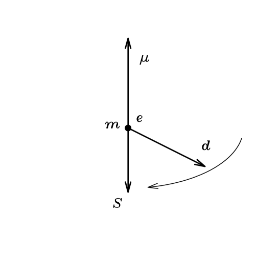
Figure 2: Approximate structure of the electron in the center of mass frame. It is a point of mass $m$ and negative charge $e$. It has a constant spin $S$ and a constant magnetic moment $\mu$ in the opposite direction, and also an oscillating electric dipole moment $d$, with frequency $\omega=2mc^{2}/\hbar\simeq 10^{21}$ s^-1, in a plane orthogonal to $S$.

If we locate mathematically a positive and negative charge $\pm e$ in the center of mass we can have an approximate structure of the classical spinning electron as a point particle of mass $m$ and charge $e$ in the center of mass of the system, with the additional electromagnetic attributes $\mu$ and $d$ as the ones depicted in figure 2. The relative orientation between the spin and magnetic moment of the classical model depends on the sign of the charge of the object considered as the particle while the antiparticle, which is described by the time reversed motion of the other and with opposite charge, will have the same relative orientation between the spin and magnetic moment, because a current in the reversed direction but of opposite charge will produce the same magnetic moment. It seems that the spin and magnetic moment of the electron are opposite to each other, which corresponds to consider that the positive charged object is the particle.

9 The Photon

In the manifold spanned by the variables $(t,{\mbox{\boldmath$r$}},{\mbox{\boldmath$v$}},\mbox{\boldmath$\alpha$})$, with $v(\tau)=c$, we have two possibilities. Since the absolute value of the velocity is always constant, then ${\mbox{\boldmath$v$}}\cdot\dot{\mbox{\boldmath$v$}}=0$. One possibility is that $\dot{\mbox{\boldmath$v$}}=0$, the particle moves in straight lines at the speed of light. We have in this case the description of a photon. The other is that $\dot{\mbox{\boldmath$v$}}\neq 0$ but always orthogonal to the velocity. This possibility leads to the electron description, as has been shown above.

For the photon, since $\dot{\mbox{\boldmath$v$}}=0$, there will be no $\dot{\mbox{\boldmath$v$}}$ term in the expansion of the Lagrangian. It is a system of six degrees of freedom. Three represent the position of a point and the other three its orientation in space and the spin will be related to the change of orientation but not to the dependence of the Lagrangian on the acceleration. The particle moves and rotates, but the Lagrangian is not a function of the acceleration, which vanishes. The homogeneity condition implies that the Lagrangian for a photon is

$$L=\epsilon\frac{S}{c}\frac{\dot{\mbox{\boldmath$r$}}\cdot\mbox{\boldmath$\omega$}}{\dot{t}},$$

where $\epsilon=\pm 1$ will be interpreted as the helicity and $S$ the absolute value of the spin, which from the classical point of view is unrestricted. The spin is now

$${\mbox{\boldmath$S$}}=\frac{\partial L}{\partial\mbox{\boldmath$\omega$}}=\epsilon S\frac{{\mbox{\boldmath$v$}}}{c},$$

which is a vector parallel ($\epsilon=+1$) or antiparallel ($\epsilon=-1$) to the velocity of propagation, and it is never transversal to the motion. Its value is independent of the observer, and thus a nonvanishing intrinsic property.

The linear momentum is

$${\mbox{\boldmath$P$}}=\frac{\partial L}{\partial\dot{\mbox{\boldmath$r$}}}=\epsilon\frac{S}{c}\,\mbox{\boldmath$\omega$},$$

in a time evolution description ($\dot{t}=1$). Since the spin is constant and $d{\mbox{\boldmath$S$}}/dt={\mbox{\boldmath$P$}}\times{\mbox{\boldmath$v$}}=0$, this means that $P$, and thus $\omega$, lie along $v$.

The energy of the photon is

$$H=-\frac{\partial L}{\partial\dot{t}}={\mbox{\boldmath$S$}}\cdot\mbox{\boldmath$\omega$},$$

and if it is definite positive both $S$ and $\omega$ have the same direction.

Because the spin structure is related to the rotation variables it can quantize with all integer and half integer values [7]. If, when quantized we take $S=\hbar$ and thus $H=\hbar\omega=h\nu$. The frequency of the photon is the frequency of its rotation around the direction of motion, leftwards or rightwards according to the spin orientation.

Because $H^{2}-{\mbox{\boldmath$P$}}^{2}c^{2}=0$, the photon is a massless system.

If, when quantized, we take for $S=\hbar/2$, we are describing both left and right handed neutrinos, but this classical formalism does not discriminate the left handed ones.

10 Conclusions

We have seen that by describing the evolution of the consecutive updated inertial observers, which measure the elementary particle in the same kinematical state, we can describe the states and dynamics of an elementary particle. Therefore we use the variables which characterize every inertial observer as the classical variables which define the kinematical state of the particle. We have found a clear interpretation between the motion of the charge at $r$ at the speed of light and the quantum mechanical Dirac analysis of the electron. Both, the magnetic and electric dipole moments, have had a clear classical explanation.

Nevertheless, the classical model has several classical inconsistencies. The stationary motion of the charge is accelerated and therefore the system has to loose energy by radiation. As an alternative, we see that although the charge is accelerated, the center of mass of the free electron is not and thus there is no variation of the kinetic energy of the free particle. It is suggesting that, from the classical viewpoint, we must revisit the classical theory of the radiation of spinning objects and associate the energy radiated with the acceleration of the center of mass. Now the model is more complex because we have to describe the evolution of two points $r$ and $q$. Alternatively, we can only describe the evolution of the center of charge $r$, but it satisfies then a fourth order differential equation, which is more difficult to analyze.

The electric field produced by this model of spinning electron it is neither static nor Coulomb like. Nevertheless its time average value during a complete turn of the charge produces an electrostatic field which is Coulomb like from a distance of three Compton’s wavelength from the origin to infinity and which does not diverge at ${\mbox{\boldmath$r$}}=0$, but it vanishes there. The time average of the magnetic field produces a static magnetic field which corresponds to the magnetic field produced by a magnetic moment $\mu$ at the origin. This static magnetic field does not diverge at the origin [7]. In this time average there is no electric dipole and this justifies the usual picture of the electron as a charged object with a magnetic moment and no electric dipole. All these fields have some infinities which go like $1/r$, and not like $1/r^{2}$, in some points of the zitterbewegung plane.

This picture predicts that the spin and magnetic moment of the particle and antiparticle have the same relative orientation. Nevertheless it is argued that for the electron they are antiparallel while they are parallel for the positron. To our knowledge, no clear experimental evidence of this relative orientation can be found in the experimental literature. Most of the very accurate measurements of the electron magnetic moment and of the $g-2$ anomaly are done by analyzing the precession frequency of the spin in external magnetic fields. But this precession frequency is independent of whether spin and magnetic moment are parallel or antiparallel vectors. Two plausible experiments for this relative measurement have been recently proposed [13].

This formalism is still at a seminal level, but some of the features it is able to describe are very promising. The usual spinless physics is contained within it. But the interest is that we can handle classical dynamical equations for spinning systems. With the use of these dynamical equations we have been able to show that there exists a nonvanishing classical probability of tunneling when the electron is properly polarized [14], and also that polarized electrons can form bound states of spin 1, and thus a gas of bosons, provided they are very close and with no very high relative velocity [10]. Spin 1 electron pairs seem to be the most probably state of condensed electrons in ferromagnetic superconductors.

Acknowlegdments

This work has been supported by the Universidad del País Vasco/Euskal Herriko Unibertsitatea research grant 9/UPV00172.310-14456/2002.

References

- [1] A.O. Barut, History of the electron, in the book: D. Hestenes and A. Weingartshofer (editors), The electron, new theory and experiment, Kluwer, Dordrecht (1991).
- [2] P.A.M. Dirac, The Principles of Quantum Mechanics, 4th ed. Oxford University Press, Oxford, (1958), section 69.
- [3] P. A. M. Dirac, Theory of electrons and positrons, Nobel Lecture, December 12, 1933, from Nobel Lectures, Physics 1922-1941, Elsevier Publishing Company, Amsterdam (1965).
- [4] P.A.M. Dirac, The Quantum Theory of the Electron, Proc. Roy. Soc. Lon. A117, 610 (1928), in particular p. 619.
- [5] E.P. Wigner, On Unitary Representations of the Inhomogeneous Lorentz Group, Ann. Math. 40, 149, (1939).
- [6] H. Bacry and J.M. Levy-Leblond, Possible Kinematics, J. Math. Phys., 9, 1605 (1968).
- [7] M.Rivas, Kinematical theory of spinning particles, Fundamental Theories of Physics Series, vol 116, Kluwer, Dordrecht (2001).
- [8] M. Rivas, Classical Particle Systems: I. Galilei free particles, J. Phys. A 18, 1971 (1985); Classical Relativistic Spinning Particles, J. Math. Phys. 30, 318 (1989); Quantization of generalized spinning particles. New derivation of Dirac’s equation, J. Math. Phys. 35, 3380 (1994). A more detailed exposition of the different models is given in [7].
- [9] J.M. Levy-Leblond, Group theoretical foundations of Classical Mechanics: The Lagrangian gauge problem, Comm. Math. Phys. 12, 64 (1969).
- [10] M. Rivas, The dynamical equation of the spinning electron, J. Phys. A, 36, 4703, (2003), and also LANL ArXiv:physics/0112005.
- [11] M. Rivas,Quantization of generalized spinning particles. New derivation of Dirac’s equation, J. Math. Phys. 35, 3380 (1994).
- [12] M. Rivas, J.M. Aguirregabiria and A. Hernández, A pure kinematical explanation of the gyromagnetic ratio of leptons and charged bosons, Phys. Lett. A 257, 21 (1999).
- [13] M. Rivas, Are the electron spin and magnetic moment parallel or antiparallel vectors?, LANL ArXiv:physics/0112057.
- [14] M. Rivas, Is there a classical spin contribution to the tunnel effect?, Phys. Lett. A 248, 279 (1998)