Constraint-defined Manifolds:
a Legacy Code Approach
to Low-dimensional Computation

Abstract

If the dynamics of an evolutionary differential equation system possess a low-dimensional, attracting, slow manifold, there are many advantages to using this manifold to perform computations for long term dynamics, locating features such as stationary points, limit cycles, or bifurcations. Approximating the slow manifold, however, may be computationally as challenging as the original problem. If the system is defined by a legacy simulation code or a microscopic simulator, it may be impossible to perform the manipulations needed to directly approximate the slow manifold. In this paper we demonstrate that with the knowledge only of a set of “slow” variables that can be used to parameterize the slow manifold, we can conveniently compute, using a legacy simulator, on a nearby manifold. Forward and reverse integration, as well as the location of fixed points are illustrated for a discretization of the Chafee-Infante PDE for parameter values for which an Inertial Manifold is known to exist, and can be used to validate the computational results.

Keywords Differential equations, inertial manifolds, stiff equations

1 Introduction

Certain dissipative evolutionary equations possess low-dimensional, attracting invariant manifolds which govern their long term dynamics. Such a manifold is readily apparent for a system given in the singularly perturbed form:

$$dy/dt=y^{\prime}=f(y,z),\hskip 14.45377ptf\in\Re^{n+m}\mapsto\Re^{n}$$

$$dz/dt=z^{\prime}=g(y,z)/\epsilon,\hskip 14.45377ptg\in\Re^{n+m}\mapsto\Re^{m}$$ (1)

where $f$ and $g$ are such that, for small positive $\epsilon$, $z$ is rapidly attracted to the region $z^{\prime}={\rm O}(1)$ and $\partial g/\partial z$ is non-singular. Since $z=z_{0}(y)+{\rm O}(\epsilon)$ where $z_{0}(y)$ is the solution of $g(y,z_{0}(y))=0$, the slow manifold is given by the solution of

$$y^{\prime}=f(y,z_{0}(y))+{\rm O}(\epsilon)$$ (2)

so that we can “easily” compute an approximation to it. The one-dimensional slow manifold is parameterized here by $y$ (other parameterizations are also possible).

In more complicated cases, approximations to the slow manifold may not be so apparent; yet within such manifolds the system dynamics can still be described by a lower-order differential equation - the reduced system. Methods for approximating such manifolds have been the subject of intense research in communities ranging from reactive flow modeling (e.g. [5, 6, 7]) to inertial manifolds for dissipative PDEs (e.g. [8, 9, 4]). If we are able to somehow constrain the dynamics to a slow manifold, stable numerical integration could be performed with larger stepsizes than would be possible in the original system. Furthermore, many global properties of the original system are (approximately) inherited by the reduced system; these include stationary points, limit cycles, and bifurcations and may be computable more easily on the slow manifold. Unfortunately, approximating the slow manifold may be as computationally challenging as the original problem.

In our work we seek an approximation to such a manifold that is (a) simple to obtain on the fly during numerical computations, and (b) only requires evaluations of time derivatives of the state, such as would be available from a legacy code. Our starting point is the assumption that, given a basis for the full set of variables in the problem, a subset of this basis can be used to parameterize the slow manifold and our approximation of it, as $y$ did in our example above. In some applications, such as when the full system is described by a microscopic simulation, the subset used to parameterize the slow manifold might be called “macroscopic observables”; such observables could be the pressure field in kinetic theory based flow simulation, or a concentration field in the kinetic Monte Carlo simulation of a chemical reaction.

We may start with a finite-dimensional system (an ODE) or an infinite-dimensional system (a PDE, for example). In the latter case we will have to introduce a finite-dimensional approximation before commencing computation (in effect, the “method of lines”). Suppose that the system is represented by (approximated by) the system

$$u_{t}=L(u)$$ (3)

where $u=\{u_{i}\},i=1,\cdots,N$. For ease of presentation, let us assume that the equation has already been transformed to a suitable basis so that $U=\{U_{i}=u_{i},\hskip 7.22743pti=1,\cdots,n\}$ parameterizes the slow manifold. In some sense we are assuming that the remaining variables, $V=\{V_{i}=u_{n+i},\hskip 7.22743pti=1,\cdots,N-n=m\}$, are the “fast” ones that are quickly “slaved” to $U$; we will return to this assumption. The split system is

$$\frac{dU}{dt}=L_{1}(U,V)$$ (4)

$$\frac{dV}{dt}=L_{2}(U,V).$$ (5)

We now view the solutions of the system as families of curves in the $U-V$ state space, as illustrated in Figure 1 - although such figures are potentially misleading because we have to remember that each axis represents a multi-dimensional space.

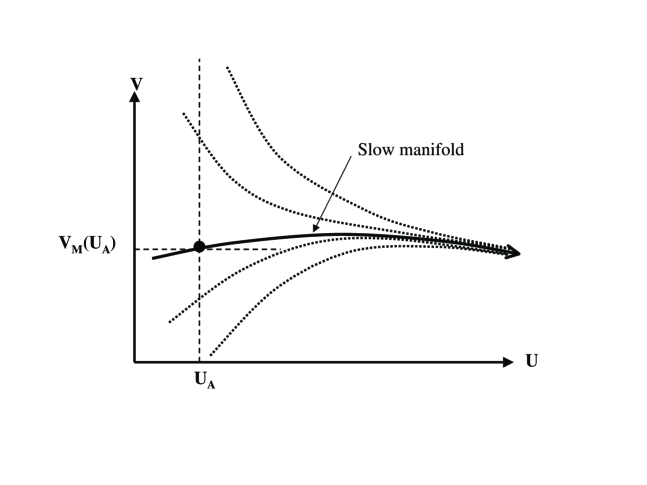
Figure 1: Family of Solutions and Slow Manifold Schematic

The essential feature of the figure is that one member of the family of solutions is a “slow” manifold with no high-curvature region, while other members of the family of solutions approach this slow manifold relatively rapidly.

Since the slow manifold, $M$, can be parameterized by the slow variables, $U$, points on $M$, $(U,V_{M}(U))$, must be uniquely determined by $U$ - that is, the curve cannot “fold” in the region of interest. If we had a scheme for approximating the value of $V=V_{M}(U)$ for each $U$ (as we did in the singularly perturbed example above) we could, for example, apply a numerical integration method to just the $U$ variables, computing the equivalent values of $V_{M}(U)$ only as needed by the integration scheme. This is the main point of our approach: one does not compute the entire manifold a priori, but only computes it pointwise, “on demand” as required by the low-dimensional integration code (or by algorithms performing other numerical tasks, such as fixed point computation).

From the assumptions, we suspect that an approximation to the slow manifold can be found by computing the value of $V=V_{A}(U)$ (as shown in Figure 2) for which the time derivatives of the $V$ components are zero. Here we will compute on this “steady manifold”; for the appropriate basis choice this steady AIM is not too far from the slow manifold. Better approximations, based on higher order expansions of singularly perturbed equations, can also be used in a legacy code context, and will be the subject of further work.

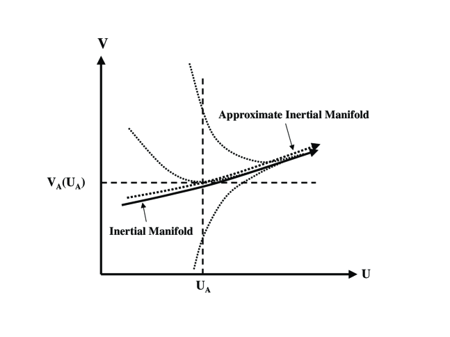
Figure 2: Approximate Inertial Manifold Definition

We are particularly interested in the case where we do not have “access” to the differential equations directly because, for example, we have a legacy simulation code, or the system is the unknown closure of a microscopic simulation model (kinetic Monte Carlo, molecular dynamics). Then, the only computational possibility we have is to integrate the full system for a short time in what we call an inner integration step. In this case, we can define an AIM by requiring that the chord of the inner step has zero change in the $V$ components, that is, it is “horizontal.” This can be computed iteratively by performing an inner integration over a small step of length $h$ and then projecting the solution back to the specified value of $U$ (by simply resetting the values of $U$ to their values at the start of the step) and repeating. If $h$ is small enough, this iteration will converge if the solution family in the neighborhood of $(U,V_{A}(U))$ is locally attracted to the solution that passes through $(U,V_{A}(U))$. This can be seen by noting that one step of the process performs the mapping

$$V_{m+1}=V_{m}+gL_{2}(U,V_{m})+{\rm O}(h^{2})$$ (6)

so we have

$$V_{m+1}-V_{m}=(I+h\frac{\partial L_{1}}{\partial V})(V_{m}-V_{m-1})+{\rm O}(h^{2})$$

which implies convergence for small enough $h$ if the eigenvalues of $\partial L_{1}/\partial V$ are in the negative half plane. This property can form the basis of alternative algorithms to approximate the “steady AIM:” matrix free fixed point algorithms, like the Recursive Projection Method or GMRES [10, 11] can be applied to accelerate the computation of the fixed point of eq. (6).

In the following sections we will illustrate the use of this technique on the Chafee-Infante reaction-diffusion equation

$$\frac{\partial u}{\partial t}=\nu\frac{\partial^{2}u}{\partial x^{2}}+u-u^{3}$$ (7)

with $\nu=(2.5)^{-2}$ and $u(0,t)=u(\pi,t)=0$. This is known to possess an inertial manifold of dimension two (in effect, the two-dimensional unstable manifold of the origin, and its closure). Although we know the differential equations in this example, we are not going to make explicit use of the knowledge in our computational method. We will only use it as if we were given a legacy code for evaluating time derivatives.

We first discretize the equations in space. Since we are not interested in the issue of the best spatial discretization, we use simple finite difference methods over $N$ equally spaced points, so that the variables are $u_{i}(t)=u(x_{i},t),i=1,\cdots,N$, where $x_{i}=\pi i/(N+1)$. These variables are chosen for convenience in the calculation. The resulting ODEs are the usual:

$$\frac{du_{i}}{dt}=\frac{\nu}{\Delta X^{2}}(u_{i-1}-2u_{i}+u_{i+1})+u_{i}-u^{3}_{i},\hskip 14.45377pti=1,\cdots,N$$ (8)

where $u_{0}=u_{N+1}=0$. If we had a legacy code or a microscopic model, the variables would be the ones that happened to come with the code or model. In this example, no subset of the $\{u_{i}\}$ variables is suitable for defining the AIM (since the slow manifold varies rapidly as a function of each $u_{i}$) so we will use an “observation basis” in which a linear combination of the variables will parameterize the AIM. In this case, we can use a basis formed by $\sin(mx),m=1,\cdots,N$. (These are the unnormalized eigenvectors of eq. (8) when $u=0$.) The modified variables are

$$a_{i}=\sum_{j=1}^{N}\phi_{ij}u_{j}\hskip 14.45377pt$$ (9)

where $\phi_{i}=\{\phi_{i*}\}$, is the basis given by $\phi_{ij}=\sin(ix_{j})$. The first two $a_{i}$ can parameterize the slow manifold, and it is not necessary to calculate the rest.

We now present a technique for approximating $d(a_{1},a_{2})/dt$ on the slow manifold given $(a_{1},a_{2})$. This approximation can then be used to implement time integration, stability analysis, or other numerical procedures on the system constrained to the AIM. The general method consists of

1. Start with a prescribed value of $(a_{1},a_{2})$.

2. Compute the values of $\{u_{i}\}$ such that eq. (9) is satisfied and the local derivative of the full ($\{u_{i}\}$ system) is “horizontal” in the other components of the basis (in this example, $a_{3},\cdots,a_{N}$). This can be done in a number of ways:

   1. Use eq. (8) and eq. (9) to compute $da_{i}/dt,3\leq i=\leq N$ and then solve for the values of $a_{j}$ that makes these zero using Newton iteration. This can be done directly when the equations are available (it is done in the example illustrated here), or can be done through matrix-free based contraction mappings if the equations are not explicitly available.

   2. If we only have a legacy code or a microscopic simulator of the full system, use iteration eq. (6) repeatedly to find the values of $a_{j},3\leq j\leq N$ such that the chords of those $a_{j}$ are zero.

   3. Conceptually (since this is not practical for a legacy code) one could implement a Lagrange multiplier, evolving the dynamics while constraining the projection of the solution on $(a_{1},a_{2})$. This is reminiscent of techniques like SHAKE used to “prepare” molecular dynamics simulations [12]. The approach described immediately above is a way of effectively implementing what amounts to such a Lagrange multiplier constrained integration to a legacy simulator.

3. Compute the derivatives (or chord slope) of the full ($\{u_{i}\}$) system from the given values of $a_{1},a_{2}$ and the now computed $a_{j},3\leq j\leq N$ (actually they have probably been computed in the previous step).

4. Compute the “$(a_{1},a_{2})$” components of the derivative by applying eq. (9) to the $\{u_{i}\}$ derivatives. These are the approximations to the time derivatives of $(a_{1},a_{2})$ on the steady AIM.

In the next section we will use this technique to integrate eq. (8) both forward and backward in time on our two-dimensional steady AIM, and compare it with the integration of the full system and in the subsequent section we will use it to compute the steady states directly by performing a Newton iteration on the two-dimensional steady AIM.

2 Integration on an AIM of the Reaction-Diffusion Equation

In [1] we introduced projective integration which uses computation of the chord slope obtained by integration of a legacy code or of a microscopic model in place of derivatives for performing large projective integration steps on the slow components. If we were working with legacy codes or microscopic simulators, we would use that technique in our “on manifold” integrations. However, we have chosen an example for which we know the equations of the detailed system, so that we can compare the “true” integration of the system with the approximation on the steady AIM we have defined.

We integrated the full system eq. (8) using the automatic Runge-Kutta method with the Dormand-Prince pair of formulae known as RK45 and available in MATLAB as ode45. We also used the same method to integrate just $(a_{1},a_{2})$ on the AIM, using the technique described in the previous section to approximate the derivatives of $(a_{1},a_{2})$. It is possibly better to view this as the (approximate) integration of the projection on the $(a_{1},a_{2})$ “observables plane” of the true dynamics. The results for $(a_{1},a_{2})$ are shown in Figure 3. The integration was started from six different points near the origin in the $(a_{1},a_{2})$ plane (which is an unstable steady state). All but one approach the stable steady state at approximately (1.12,0) but the one that starts at (0,0.05) stays on the invariant submanifold $a_{1}=0$ and moves to the saddle point at about (0,0.7). Since the origin is on the inertial manifold of eq. (8), the starting points are also very close to it so that the RK45 integration of the full system gives a good approximation of the solutions on the inertial manifold and provides a picture of the manifold itself. In Figure 3, the solid line is the RK45 solution of the full system, while the dashed line is the integration on our steady AIM.

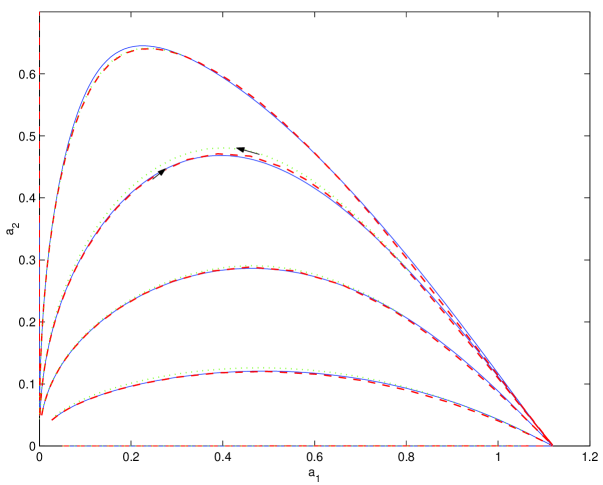
Figure 3: Trajectories in $(a_{1},a_{2})$-plane. Solid: Inertial manifold, dashed - AIM forward, dotted - AIM reverse.

The full system in eq. (8) is rapidly damped in its fastest components, and so it would not be feasible to numerically integrate it in the reverse time direction. However, the $(a_{1},a_{2})$ differential system on the AIM does not have these fast components, so it can be integrated “backwards.” The dotted arcs in Figure 3 are the results of a reverse integration in the $(a_{1},a_{2})$-plane starting from a point on the RK45 solution of the full system shortly before the stationary point is reached (one can’t start too close to the stationary point because the trajectory chosen would be too sensitive to small perturbations).

As we can see in Figure 3, the forward and reverse solutions on the AIM are fairly good approximations to the components of the “true” solution on the IM. We do not expect the other components, $a_{i},i\geq 3$ to be good approximations. This is shown in Figure 4 which shows the values of $a_{3}$ plotted against $a_{1}$ for each of the trajectories. (The reverse integration trajectories are almost indistinguishable from the forward trajectories for the $(a_{1},a_{2})$ integration.)

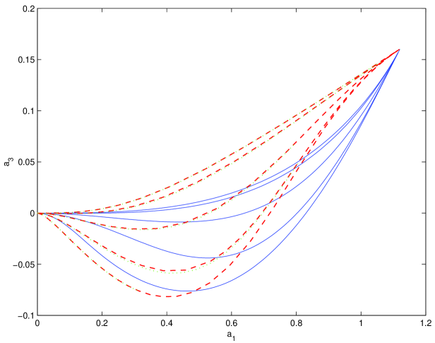
Figure 4: $(a_{1},a_{3})$ trajectories. Solid: Inertial manifold, dashed - AIM forward, dotted - AIM reverse.

3 Steady State Computation on the AIM

The procedure described in Section 1 computes $da/dt=p(a)$ where $a=(a_{1},a_{2})$ is the parameterization of the slow manifold. Using any standard techniques we can look for zeros of $p(a)$ to identify stationary states of the system. Since the dimension is low, we can use Newton’s method, computing the approximate partial derivatives by finite differencing. Many better methods exist, but our purpose here is simply to show that the reduced system can be used directly in any conventional numerical process.

Table 1 shows the sequence of iterates for Newton’s method starting at three different point in the $(a_{1},a_{2})$-plane and iterating until changes were less than $10^{-5}$ in the L1 norm. The eigenvalues of $J=\partial p/\partial a$ as the iteration proceeds are also shown. For comparison, the two leading eigenvalues of the full system eq. (8) at steady state for each of the three cases are (0.8403,0.3648), (0.2204,-0.7118), and (-1.4491,-1.5392) respectively. As can be seen, the three stationary points, (0,0), (0,0.7056), and (1.1206,0) are source, saddle, and stable (sink), respectively. Note that the stationary states on the steady AIM are necessarily on the slow manifold since all of the derivatives are zero at these points.

Table 1: Sequence of Newton Iterates

Case 1
$a_{1}$	$a_{2}$	$\lambda_{1}$	$\lambda_{2}$
0.2000	0.2000	0.7171	0.1971
-0.0838	-0.1946	0.7737	0.2684
0.0159	0.0551	0.8351	0.3571
-0.0002	-0.0009	0.8403	0.3648
0.0000	0.0000	0.8403	0.3648
Case 2
$a_{1}$	$a_{2}$	$\lambda_{1}$	$\lambda_{2}$
0.1000	0.7500	0.1666	-0.8904
-0.0405	0.7271	0.2069	-0.7902
0.0063	0.7087	0.2359	-0.7293
-0.0001	0.7057	0.2405	-0.7203
0.0000	0.7056	0.2407	-0.7200
Case 3
$a_{1}$	$a_{2}$	$\lambda_{1}$	$\lambda_{2}$
1.0000	0.1000	-0.8687	-1.5201
1.1707	-0.0462	-2.0297	-1.6832
1.1255	-0.0042	-1.6847	-1.6599
1.1206	-0.0000	-1.6529	-1.6529
1.1206	-0.0000	-1.6528	-1.6526

4 Discussion

We have demonstrated that it is possible to perform low-dimensional (macroscopic) computations on an AIM (more precisely, on observations of an AIM) based on choosing a suitable parameterization of the low dimensional slow manifold. That parameterization must be chosen so that the slow manifold does not “fold over it”. It must also be chosen so that the induced AIM is reasonably close to the true slow manifold. In the example we discussed, the first two eigenvectors of the linearization of the problem at a particular solution value (the origin) were chosen to parameterize the manifold, since at that solution value they are tangent to the true slow manifold. As long as the solution does not stray too far from that region (compared to the non-linearities present) these directions provide a reasonable parameterization to the slow manifold elsewhere. The steady AIM for these two variables is illustrated in Figure 5 which plots $a_{3}$ against $a_{1}$ and $a_{2}$ on the AIM. This AIM is a reasonable approximation of the slow manifold, (which is shown is Figure 1 of [13]). It is clear from this figure that choosing, say, $a_{2}$ and $a_{3}$ to characterize the slow manifold would have been bad since $a_{1}(a_{2},a_{3})$ is multivalued for some $a_{3}$. (See the line $a_{2}=1,a_{3}=-0.1$ that is indicated in the figure. It intersects the AIM twice within the region plotted.) This is true even near the origin, where this AIM is a good approximation to the inertial manifold.

The focus of this work was on the use of a legacy simulator to approximate the slow manifold on the fly, as dictated by the needs of numerical analysis tools employed for computations on it. The local nature of the approximation should be contrasted to “off line” algorithms that attempt to approximate the entire manifold first (see the extensive discussion in [14] as well as [15]). Here we pursued the simplest approximate manifold one can find by constraining a legacy code. An important issue that was only tangentially mentioned here was the selection of good basis functions (or macroscopic observables in the case of atomistic inner simulators) that parameterize the manifold; statistical data analysis techniques have an important role to play in this. Better algorithms, resulting from the implementation of higher order approximations to the slow manifold (requiring a higher order derivative to vanish) in a legacy code context are currently being explored.

Acknowledgements This work was partially supported by an NSF/ITR grant and by the AFOSR Dynamics and Control (Dr. B. King).

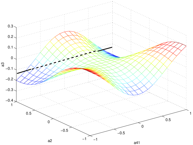
Figure 5: $a_{3}$ as a function of $a_{1}$ and $a_{2}$ on the AIM.

References

- [1] Gear, C. W. and Kevrekidis, I. G. “Projective Methods for Stiff Differential Equations: problems with gaps in their eigenvalue spectrum”; NEC Technical Report NECI-TR 2001-029 SIAM J. Sci. Comp.. 24(4) pp.1091-1106 (2003).
- [2] Gear, C. W. and Kevrekidis, I. G. “Computing in the Past with Forward Integration”, Physics Letters A in press (2003). Can be obtained as nlin.CD/0302055 at arXiv.org
- [3] Rico-Martinez, R., C. W. Gear and I.G.Kevrekidis “Coarse Projective kMC Integration: Forward/Reverse Initial and Boundary Value Problems”, J. Comp. Phys., in press (2003); can be found as nlin.CG/0307016 at arXiv.org.
- [4] M. S. Jolly, I. G. Kevrekidis and E. S. Titi “Approximate Inertial Manifolds for the Kuramoto-Sivashinsky Equation: Analysis and Computations”, Physica D, 44 pp.38-60 (1990).
- [5] U. Maas and S. B. Pope “Simplifying chemical kinetics: Intrinsic Low-Dimensional Manifolds in Composition Space” Combustion and Flame 88 (1992) pp.239-264.
- [6] S. H. Lam and D. A. Goussis “The CSP method for simplifying chemical kinetics” Int. J. Chem. Kin. 26 pp.461-486 (1994)
- [7] A. N. Gorban and I. V. Karlin “Method of invariant manifolds for chemical kinetics” arXiv:cond-mat/0207231
- [8] P. Constantin, C. Foias, B. Nicolaenko and R. Temam Integral manifolds and inertial manifolds for dissipative partial differential equations New York, Springer (1988)
- [9] R. Temam Infinite Dimensional Dynamical Systems in Mechanics and Physics New York, Springer (1988)
- [10] Shroff, G.M. and Keller, H.B. “Stabilization of unstable procedures: A recursive projection method”, SIAM J. Numer. Anal. 30, 1099-1120. (1993)
- [11] C. T. Kelley, Iterative Methods for Linear and Nonlinear Equations, SIAM Publications, Philadelphia (1995)
- [12] J. P.Ryckaert, G. Ciccotti and H. Berendsen “Numerical Integration of the Cartesian equations of motion of a system with constraints: Molecular Dynamics of N-alkanes” J. Comp. Phys. 23 pp.327-341 (1977)
- [13] C. Foias, M. S. Jolly, I.G. Kevrekidis, G. R. Sell and E. S. Titi “On the computation of inertial manifolds” Phys. Letters A 131 pp.433-436 (1988)
- [14] A. N. Gorban, I. V. Karlin and Yu. Zinoviev “Constructive methods of invariang manifolds for kinetic problems” IHES Report M/03/50, July 2003.
- [15] D. A. Jones and E. S. Titi “Approximations of inertial manifolds for dissipative nonlinear equations” J. Diff. Equ. 127 pp.54-86 (1996)