Also at P.N. Lebedev Physics Institute, Moscow, Russia]   Also at Ludwig-Maximilians-University, Munich, Germany]

New Limits on the Drift of Fundamental Constants from Laboratory Measurements

Abstract

We have remeasured the absolute $1S$-$2S$ transition frequency $\nu_{\rm{H}}$ in atomic hydrogen. A comparison with the result of the previous measurement performed in 1999 sets a limit of $(-29\pm 57)$ Hz for the drift of $\nu_{\rm{H}}$ with respect to the ground state hyperfine splitting $\nu_{{\rm{Cs}}}$ in ¹³³Cs. Combining this result with the recently published optical transition frequency in ¹⁹⁹Hg⁺ against $\nu_{\rm{Cs}}$ and a microwave ⁸⁷Rb and ¹³³Cs clock comparison, we deduce separate limits on $\dot{\alpha}/\alpha=(-0.9\pm 2.9)\times 10^{-15}$ yr^-1 and the fractional time variation of the ratio of Rb and Cs nuclear magnetic moments $\mu_{\rm{Rb}}/\mu_{\rm{Cs}}$ equal to $(-0.5\pm 1.7)\times 10^{-15}$ yr^-1. The latter provides information on the temporal behavior of the constant of strong interaction.

In the era of a rapid development of precision experimental methods, the stability of fundamental constants becomes a question of basic interest. Any drift of non-gravitational constants is forbidden in all metric theories of gravity including general relativity. The basis of these theories is Einstein’s Equivalence Principle (EEP) which states that weight is proportional to mass, and that in any local freely falling reference frame, the result of any non-gravitational experiment must be independent of time and space. This hypothesis can be proven only experimentally as no theory predicting the values of fundamental constants exists. In contrast to metric theories, string theory models aiming to unify quantum mechanics and gravitation allow for, or even predict, violations of EEP. Limits on the variation of fundamental constants might therefore provide important constraints on these new theoretical models.

A recent analysis of quasar absorption spectra with redshifted UV transition lines indicates a variation of the fine structure constant $\alpha=e^{2}/4\pi\varepsilon_{0}\hbar c$ on the level of $\Delta\alpha/\alpha=(-0.54\,\pm\,0.12)\times 10^{-5}$ for a redshift range $(0.2<z<3.7)$ Mur03 (1). On geological timescales, a limit for the drift of $\alpha$ has been deduced from isotope abundance ratios in the natural fission reactor of Oklo, Gabon, which operated about $2$ Gyr ago. Modeling the processes which have changed the isotope ratios of heavy elements gives a limit of $\Delta\alpha/\alpha=(-0.36\,\pm\,1.44)\times 10^{-8}$ Fuj00 (2). In these measurements, the high sensitivity to the time variation of $\alpha$ is achieved through very long observation times at moderate resolution for $\Delta\alpha$. Therefore, they are vulnerable to systematic effects Uzan (3).

Laboratory experiments can reach a $10^{-15}$ accuracy within years with better controlled systematics. This type of experiment is typically based on repeated absolute frequency measurements, i.e. comparison of a transition frequency with the reference frequency of the ground state hyperfine transition in ¹³³Cs. For an optical transition, the theoretical expression for the drift of its absolute frequency inevitably involves $\mu_{\rm{Cs}}/\mu_{B}$ in addition to $\alpha$, where $\mu_{\rm{Cs}}$ is the magnetic moment of the Cs nucleus and $\mu_{B}$ is the Bohr magneton Karsh (4). The microwave Rb and Cs clock comparison Mar03 (5) even involves two nuclear moments. The magnitude of nuclear moments results from both the electromagnetic and the strong interaction.

Contributions from weak, electromagnetic, and strong interactions can be disentangled by combining several frequency measurements possessing a different sensitivity to the fundamental constants. In this letter, we deduce separate stringent limits for the drifts of the fine structure constant $\alpha$, $\mu_{\rm{Cs}}/\mu_{B}$ and $\mu_{\rm{Rb}}/\mu_{\rm Cs}$ from combining the drifts of two optical frequencies in hydrogen and in the mercury ion with respect to the ground state hyperfine splitting in ¹³³Cs and the result of a microwave clock comparison Mar03 (5). Comparing measurements performed at different places and at different times we have to use the Lorentz and position invariance and we have to assume that the constants change linearly and do not oscillate on a year scale. With exception of this, our results are independent of further assumptions about a particular drift model and possible correlated drifts of different constants Cal02 (6).

The experiments on the drift of the ¹⁹⁹Hg⁺ $5d^{10}6s\ {{}^{2}}S_{1/2}(F=0)\rightarrow 5d{{}^{\,9}}6s^{2}\,{{}^{2}}D_{5/2}(F^{\prime}=2)$ electric quadrupole (“clock”) transition frequency $\nu_{\rm{Hg}}$ were performed by the group of J. Bergquist at NIST between July 2000 and December 2002 Biz03 (7). These repeated measurements of $\nu_{\rm{Hg}}$ limit the fractional time variation of the ratio $\nu_{\rm{Cs}}/\nu_{\rm{Hg}}$ to $(0.2\pm 7)\times 10^{-15}$ yr^-1.

In 1999 Nie00a (8) and 2003, we have phase coherently compared the frequency of the $(1S,F\!\!=\!\!1,m_{F}\!\!=\!\!\pm 1)\rightarrow(2S,F^{\prime}\!\!=\!\!1,m_{F}^{\prime}\!\!=\!\!\pm 1)$ two-photon transition in atomic hydrogen to the frequency of the ground state hyperfine splitting of ¹³³Cs using a frequency comb technique Rei00a (9). The 1999 setup of the hydrogen spectrometer has been described previously in Hub98b (10), so we present only a brief description with emphasis on the improvements since 1999. A sketch of the actual setup is shown in Fig.1.

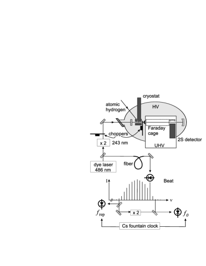
Figure 1: Simplified experimental setup for comparison of the hydrogen $1S$-$2S$ transition frequency with a primary frequency standard (HV: high vacuum, UHV: ultra-high vacuum). A mode-locked femtosecond laser with repetition rate $f_{\rm rep}$ emits the frequency comb which is broadened in a photonic crystal fiber. $f_{0}$ is the carrier-envelope offset frequency.

A cw dye laser emitting near 486 nm is locked to an external reference cavity. The new cavity for the 2003 measurement is more stable and drifts less than 0.5 Hz/s at 486 nm. The linewidth of the dye laser stabilized on the new cavity has been characterized as 60 Hz for an averaging time of 1 s. A small part of the laser light is transferred to a neighboring lab where its absolute frequency is measured. The main part is frequency doubled, and the resulting radiation near 243 nm (corresponding to half of the $1S$-$2S$ transition frequency) is coupled into a linear enhancement cavity inside the vacuum chamber of the hydrogen spectrometer.

Hydrogen atoms from a radio-frequency (rf) gas discharge are cooled to 5-6 K by collisions with the walls of a copper nozzle. The nozzle forms a beam of cold atomic hydrogen which leaves the nozzle collinearly with the cavity axis and enters the interaction region between the nozzle and the detector shielded from stray electric fields by a Faraday cage. Some of the atoms are excited from the ground state to the metastable $2S$ state by Doppler-free absorption of two counter-propagating photons from the laser field in the enhancement cavity. The 1999 measurement was performed at a background gas pressure of around $10^{-6}$ mbar in the interaction region. In the meantime, we upgraded the vacuum system with a differential pumping configuration. This allows us to vary the background gas pressure in a range of $10^{-8}$-$10^{-7}$ mbar and to reduce the background gas pressure shift and the corresponding uncertainty to 2 Hz.

Due to small apertures, only atoms flying close to the cavity axis can enter the detection region where the $2S$ atoms are quenched in a small electric field and emit $L_{\alpha}$-photons. The excitation light and the hydrogen beam are periodically blocked by two mutually phase locked choppers, and the $L_{\alpha}$-photons are counted time-resolved only in the dark part of a cycle. The delay $\tau$ between blocking the 243 nm radiation and the start of photon counting sets the upper limit for the atomic velocity of $v<l/\tau$, where $l$ is the distance between nozzle and detector. With the help of a multi-channel scaler, we count all photons and sort them into 12 adjacent time bins. From each scan of the laser frequency over the hydrogen $1S$-$2S$ resonance we therefore get up to 12 spectra measured with different delays. To correct for the second order Doppler shift, we use an elaborate theoretical model to fit all the delayed spectra of one scan simultaneously with a set of 7 fit parameters Hub98b (10). The result of the fitting procedure is the $1S$-$2S$ transition frequency for a hydrogen atom at rest.

The transition frequency depends linearly on the excitation light intensity due to the dynamic AC-Stark shift. We vary the intensity and extrapolate the transition frequency to zero intensity to correct for this effect Nie00a (8).

For an absolute measurement of the $1S$-$2S$ transition frequency, the dye laser frequency near 616.5 THz is phase coherently compared with an atomic cesium fountain clock. We take advantage of the frequency comb technique recently developed in Garching and Boulder Rei00a (9) to bridge the large gap between the optical and radio frequency domains. A mode locked femtosecond (fs) laser emits a pulse train which equals a comb of laser modes in the frequency domain. The mode spacing corresponds to the repetition rate frequency $f_{\rm rep}$ of the fs laser, and the frequency of each mode can be written as $f_{n}=nf_{\rm rep}+f_{0}$, where $n$ is a large integer number and $f_{0}<f_{\rm rep}$ is the comb offset frequency. The repetition rate $f_{\rm rep}$ can easily be detected with a photodiode. For combs spanning more than one octave, $f_{0}$ can be determined by frequency doubling an infrared mode $f_{n}$ in a nonlinear crystal to $2f_{n}$ and measuring the beat note with the appropriate mode $f_{2n}$ of the blue part of the comb, yielding $f_{0}=2f_{n}-f_{2n}$.

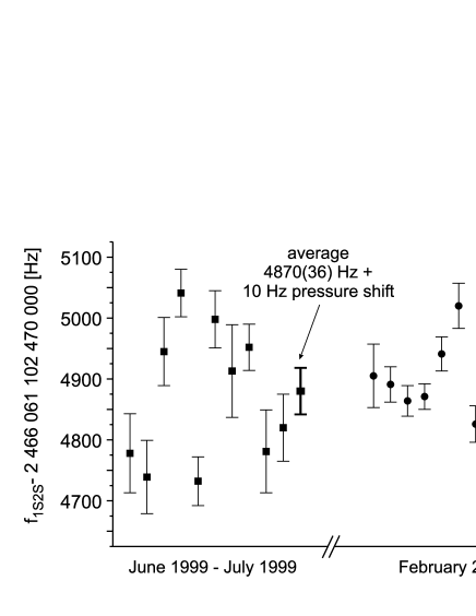
Figure 2: Experimental results and averages for the 1999 and 2003 measurements of the absolute $(1S,F\!=\!1,m_{F}=\pm 1)\rightarrow(2S,F^{\prime}\!=\!1,m^{\prime}_{F}=\pm 1)$ transition frequency in atomic hydrogen. The background pressure shift of +10 Hz as explained in Nie00a (8) is added to the 1999 value.

In our experiment, the frequency comb from a mode-locked fs Ti:Sapphire laser with a repetition rate $f_{\rm rep}$ of 800 MHz is broadened in a photonic crystal fiber to cover more than an optical octave. We phase lock both degrees of freedom of the comb ($f_{\rm rep}$, $f_{0}$) to the radio frequency output of the Cs fountain clock to get a frequency comb with optical modes whose frequencies are known with the accuracy of the primary frequency standard. Any of these modes is available for optical measurements.

For both the 1999 and 2003 measurements, the transportable Cs fountain clock FOM has been installed at MPQ. Its stability is $1.8\times 10^{-13}\tau_{\rm ave}^{-1/2}$ for an averaging time $\tau_{\rm ave}$ and its accuracy has been evaluated to $8\times 10^{-16}$ Abg03 (11) at BNM-SYRTE. During the experiments in Garching, only a verification at the level of $10^{-15}$ has been performed. Consequently we attribute a conservative FOM accuracy of $2\times 10^{-15}$ for these measurements.

We have measured the $1S$-$2S$-transition in atomic hydrogen during 10 days in 1999 and during 12 days in 2003. For comparability, both data sets have been analyzed using the same theoretical line-shape model Hub98b (10). In Fig.2, the results of the extrapolation to zero excitation light intensity and the respective statistical error bars for each day are presented. The statistical uncertainty was significantly reduced compared to the 1999 measurements due to the narrower laser linewidth and a better signal-to-noise ratio, but the scatter of the day averages did not reduce accordingly. We ascribe this effect to a residual uncompensated first-order Doppler shift. Later measurements performed without the fountain clock with a deliberately introduced asymmetry in the 243 nm cavity indicate an adjustment-dependent frequency shift (the elimination of this additional systematic shift should be of high concern in future measurements). The effect should average out after multiple re-adjustments of the spectrometer which have been typically performed twice a day. It is impossible to correct the data a posteriori because such details of the spectrometer adjustment were not recorded during the phase-coherent measurement. Other effects which can cause the systematic shift (intra-beam pressure shift, background gas pressure shift, Stark shift of the hyperfine levels induced by the rf gas discharge, stray electric fields) have been checked and can be excluded on the level of the observed scatter.

The 1999 and 2003 day-dependent data were averaged without weighting remark (12). After accounting for the total systematic uncertainties of 28 Hz (1999) and 23 Hz (2003) in the mutually equivalent evaluation processes of both measurements we deduce a difference equal to $(-29\pm 57)$ Hz over a time interval of 44 months. This is equivalent to a fractional time variation of the ratio $\nu_{\rm Cs}/\nu_{\rm H}$ equal to $(3.2\pm 6.3)\times 10^{-15}$ yr^-1.

The frequency of any optical transition can be written as $\nu=A\,Ry\,F_{\rm rel}(\alpha)$ Dzu99 (14, 4), where $Ry$ is the Rydberg energy and the relativistic correction $F_{\rm rel}(\alpha)$ takes into account relativistic and many-body effects. $F_{\rm rel}$ depends on the transition in the system considered and embodies the dependence on $\alpha$, while the parameter $A$ is independent of fundamental constants. For absolute frequency measurements $Ry$ always cancels out.

Numerical calculations of the dependence of $F_{{\rm rel},{\rm{Hg}}}(\alpha)$ for $\nu_{\rm{Hg}}$ on the fine structure constant $\alpha$ yield Dzu99 (14)

$$\alpha\frac{\partial}{\partial\alpha}\ln F_{{\rm rel},{\rm{Hg}}}(\alpha)\approx\frac{\alpha}{\Delta\alpha}\frac{\Delta F_{\rm rel}}{F_{\rm rel}}=-3.2\,.$$ (1)

The corresponding expression for $\nu_{\rm{H}}$ gives a very weak dependence on $\alpha$:

$$\alpha\frac{\partial}{\partial\alpha}\ln F_{{\rm rel},{\rm{H}}}(\alpha)\approx 0\,.$$ (2)

The frequency of the ground state hyperfine transition in ¹³³Cs is given by

$$\nu_{\rm{Cs}}=A^{\prime}\,Ry\,\alpha^{2}\,\frac{\mu_{\rm{Cs}}}{\mu_{B}}\,F_{{\rm rel},{\rm{Cs}}}(\alpha).$$ (3)

Following Dzu99 (14), the relativistic correction $F_{{\rm rel},{\rm{Cs}}}(\alpha)$ is

$$\alpha\frac{\partial}{\partial\alpha}\ln F_{{\rm rel},{\rm{Cs}}}(\alpha)\approx+0.8\,.$$ (4)

Therefore, the comparison of the clock transition in Hg⁺ against a primary frequency standard tests a drift of Biz03 (7)

$$\frac{\partial}{\partial t}\ln\frac{\nu_{\rm Cs}}{\nu_{\rm Hg}}=\frac{\partial}{\partial t}\left(\ln\frac{\mu_{\rm Cs}}{\mu_{B}}+(2.0+0.8+3.2)\ln\alpha\right)\,,$$ (5)

whereas the $1S$-$2S$ experiment tests the drift of

$$\frac{\partial}{\partial t}\ln\frac{\nu_{\rm Cs}}{\nu_{\rm H}}=\frac{\partial}{\partial t}\left(\ln\frac{\mu_{\rm Cs}}{\mu_{B}}+(2.0+0.8)\ln\alpha\right)\,.$$ (6)

For clarity, we set $x\equiv\frac{\partial}{\partial t}\ln\alpha$, $y\equiv\frac{\partial}{\partial t}\ln\frac{\mu_{\rm{Cs}}}{\mu_{B}}$ and get as experimental constraints

$$y+6x = (0.2\pm 7)\times 10^{-15}\ \textrm{yr}^{-1}\ \ \textrm{ (Hg}^{+}\textrm{),}$$ (7a)

$$y+2.8x = (3.2\pm 6.3)\times 10^{-15}\ \textrm{yr}^{-1}\ \ \textrm{ (H).}$$ (7b)

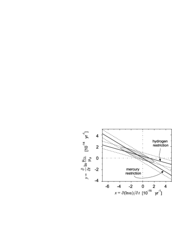
Figure 3: Possible values for the relative drift rates $x$ and $y$ and their experimental restrictions (dashed lines) as stated by eqns. (7). The probability density for $x$ and $y$ to be the true values is given by $P(\Delta x,\,\Delta y)\propto\exp[-R(\Delta x,\,\Delta y)/2]$ with the distances from the crossing point $\Delta x$ and $\Delta y$ and $R(\Delta x,\,\Delta y)=(\Delta y+6\Delta x)^{2}/\sigma^{2}_{\rm Hg}+(\Delta y+2.8\Delta x)^{2}/\sigma^{2}_{\rm H}$. The resulting elliptical uncertainty region, defined by $R(\Delta x,\,\Delta y)=1$, gives the standard deviation when projected on either axis by integration over the other. The uncertainties of the measured values are $\sigma_{\rm H}=6.3\times 10^{-15}$ yr^-1 and $\sigma_{\rm Hg}=7\times 10^{-15}$ yr^-1.

Solving for $x$ and $y$ yields the separate restrictions for the drifts of $\alpha$ and $\mu_{\rm{Cs}}/\mu_{B}$ without any assumptions of conceivable mutual correlations (see e.g. Cal02 (6)). In this sense, this evaluation is model-independent. Figure 3 represents both equations and their solution graphically.

For the relative drift of the fine structure constant at the end of the second millennium, we deduce the limit of

$$x=\frac{\partial}{\partial t}{\ln\alpha}=(-0.9\pm 2.9)\times 10^{-15}\ {\rm yr}^{-1}.$$ (8)

The limit on the relative drift of $\mu_{\rm{Cs}}/\mu_{B}$ is

$$y=\frac{\partial}{\partial t}\ln\frac{\mu_{\rm{Cs}}}{\mu_{B}}=(0.6\pm 1.3)\times 10^{-14}\ {\rm yr}^{-1}.$$ (9)

We deduce the uncertainties in expressions (8) and (9) as projections of the ellipse (Fig. 3) on the corresponding axes. This is equivalent to performing Gaussian propagation of uncertainties when resolving Eqs. (7) for $x$ and $y$. Here, the measurement results for Hg⁺ and H are treated as uncorrelated even though the drift rates $x$ and $y$ may be correlated Cal02 (6). The given $1\sigma$-uncertainties for $x$ and $y$ in Eqs. (8) and (9) incorporate both the statistical and systematic uncertainties of the hydrogen and the mercury measurements. Both limits (8) and (9) are consistent with zero. Meanwhile E. Peik and coworkers have added a precise drift measurement on a single trapped Yb ion to push the overall limit even further Peik (13).

These results allow us to deduce a restriction for the relative drift of the nuclear magnetic moments in ⁸⁷Rb and ¹³³Cs. From 1998 to 2003, the drift of the ratio of the ground state hyperfine frequencies in ⁸⁷Rb and ¹³³Cs has been measured to be Mar03 (5)

$$\frac{\partial}{\partial t}\ln\frac{\nu_{\rm{Rb}}}{\nu_{\rm{Cs}}}=(0.2\pm 7.0)\times 10^{-16}\ \textrm{ yr}^{-1}.$$ (10)

Substituting the corresponding dependencies $F_{\rm rel}(\alpha)$ for these transitions Mar03 (5, 14) yields

$$\frac{\partial}{\partial t}\ln\frac{\nu_{\rm{Rb}}}{\nu_{\rm{Cs}}}=\frac{\partial}{\partial t}\left(\ln\frac{\mu_{\rm{Rb}}}{\mu_{\rm{Cs}}}-0.53\ln\alpha\right).$$ (11)

Combining (8), (10), and (11) we get

$$\frac{\partial}{\partial t}\ln\frac{\mu_{\rm{Rb}}}{\mu_{\rm{Cs}}}=(-0.5\pm 1.7)\times 10^{-15}\ \textrm{ yr}^{-1},$$ (12)

where the same procedure as in Fig.3 was used with a diagram covering $x$ and $z\equiv\frac{\partial}{\partial t}\ln(\mu_{\rm Rb}/\mu_{\rm Cs})$.

In conclusion, we have determined separate limits for the drift of $\alpha$, $\mu_{\rm{Cs}}/\mu_{B}$ and $\mu_{\rm{Rb}}/\mu_{\rm{Cs}}$ from laboratory experiments without assumptions of conceivable correlations among them. All these limits are consistent with zero. Quasar absorption spectra measured with the Keck/HIRES spectrograph show a significant deviation between the values of $\alpha$ today and 10 Gyr ago Mur03 (1). A corresponding linear drift of $\alpha$ is smaller than the uncertainty of our result, therefore it cannot be excluded.

We thank S.G. Karshenboim for fruitful discussions of this work. N.K. acknowledges support from the AvH Stiftung. The work was partly supported by DFG (grant No. 436RUS113/769/0-1) and RFBR. The development of the FOM fountain was supported by Centre National d’études spatiales and Bureau National de Métrologie.

References

- (1) M. T. Murphy, J. K. Webb, V. V. Flambaum, astro-ph/0306483; see also J. K. Webb et al., Phys. Rev. Lett. 87, 091301 (2001).
- (2) Y. Fujii et al., Nuc. Phys. B 573, 377 (2000).
- (3) J.-P. Uzan, Rev. Mod. Phys. 75, 403 (2003).
- (4) S. G. Karshenboim, Can. J. Phys. 78, 639 (2000); see also physics/0306180.
- (5) H. Marion et al., Phys. Rev. Lett. 90, 150801 (2003).
- (6) X. Calmet, H. Fritzsch, Eur. Phys. J. C 24, 639 (2002).
- (7) S. Bize et al., Phys. Rev. Lett. 90, 150802 (2003).
- (8) M. Niering et al., Phys. Rev. Lett. 84, 5496 (2000).
- (9) Th. Udem, R. Holzwarth, and T.W. Hänsch, Nature 416, 233 (2002).
- (10) A. Huber et al., Phys. Rev. A 59, 1844 (1999).
- (11) M. Abgrall, Thèse de doctorat de l’université Paris VI (2003).
- (12) The result presented in Nie00a (8) was inadvertently described as “the weighted mean value” but was calculated without consideration of day-averaged uncertainties.
- (13) E. Peik et al., physics/0402132, also to appear in PRL.
- (14) V.A. Dzuba, V.V. Flambaum, and J.K. Webb, Phys. Rev. A 59, 230 (1999); V.V. Flambaum, physics/0302015.