Sensitive dependence on initial conditions in transition to turbulence in pipe flow

Abstract

The experiments by Darbyshire and Mullin (J. Fluid Mech. 289, 83 (1995)) on the transition to turbulence in pipe flow show that there is no sharp border between initial conditions that trigger turbulence and those that do not. We here relate this behaviour to the possibility that the transition to turbulence is connected with the formation of a chaotic saddle in the phase space of the system. We quantify a sensitive dependence on initial conditions and find in a statistical analysis that in the transition region the distribution of turbulent lifetimes follows an exponential law. The characteristic mean lifetime of the distribution increases rapidly with Reynolds number and becomes inaccessibly large for Reynolds numbers exceeding about 2200. Suitable experiments to further probe this concept are proposed.

1 Introduction

The transition to turbulence in pipe flow has been the subject of many investigations since the first documentation of its phenomenology in Reynolds (1883). Reynolds already noticed that there was no sharp transition, that the transition could be delayed to very high Reynolds number when perturbations to the laminar profile were carefully avoided and that sometimes turbulence appeared without clear evidence for a perturbation that may have triggered it. His findings have been confirmed and expanded on in many subsequent experiments, e.g. Wygnanski & Champagne (1973); Wygnanski et al. (1975); Rubin et al. (1980); Eggels et al. (1994); Ma et al. (1999); Darbyshire & Mullin (1995). On the theoretical side, no linear instability could be found (see Schmid & Henningson (1994); Meseguer & Trefethen (2003) and references therein) but analysis of the consequences of the non-normality of the linearized problem has led to the identification of efficient amplification mechanisms that can explain the sensitivity to small perturbations of the laminar profile Boberg & Brosa (1988); Schmid & Henningson (1994); Trefethen et al. (2000, 1993); Grossmann (2000); Hof et al. (2003). On the other hand the simulations in Brosa (1989) and the experiments in Darbyshire & Mullin (1995) suggest that even if the perturbations are large enough to trigger turbulence, the flow can re-laminarize without any previous indication. Similar behaviour has been found in plane Couette flow Schmiegel & Eckhardt (1997, 2000); Bottin et al. (1998); Faisst & Eckhardt (2000); Eckhardt et al. (2002).

Decay of the turbulent flow must follow from the dynamics of the fully developed 3-d turbulent state and cannot be explained by linearization around the laminar flow. The dynamical system concept compatible with such a behaviour is that of a chaotic saddle, a transient object with chaotic dynamics Tél (1991); Ott (1993). The simplest example of a chaotic saddle arises for a particle in a box with a tiny hole: the dynamics inside the box can be chaotic, as measured by positive Lyapunov exponents, but it is transient and ends when the particle leaves through the hole. The escape through the hole is a global event, and its rate is not related to the Lyapunov exponent. The analogy then is that the turbulent state is motion in the box, and escape from the box is related to relaminarization. The characteristic signatures of a chaotic saddle are: (a) a sensitive dependence of lifetimes on initial conditions, (b) an exponential distribution of lifetimes for initial conditions around the chaotic saddle, (c) a positive Lyapunov exponent in the chaotic phase, and (d) an independence of the variations of Lyapunov exponents and the escape rates with parameters. We will show here that the transition to turbulence in pipe flow shows all these characteristics and is thus compatible with the formation of a chaotic saddle.

Our analysis is based on numerical simulations of the time evolution of perturbations in circular pipe flow with periodic boundary conditions in the downstream direction. The axial periodicity length will be too short to simulate localized turbulent structures, such as puffs and slugs Wygnanski & Champagne (1973); Wygnanski et al. (1975), but long enough to capture the local turbulent structures. Following the simulations of Eggels et al. (1994) we take a length $10R$, with $R$ the pipe radius. The turbulence will then typically fill the entire volume and we do not have to consider the advection of the turbulent state by the mean profile: lifetimes can be defined locally. The Reynolds number $Re$ is based on the mean streamwise flow velocity $U$ and the pipe diameter $2R$,

$$Re=2RU/\nu\,.$$ (1)

and the units of time are $2R/U$. As in the experiments Darbyshire & Mullin (1995) we keep the volume flux constant in time: this simplifies the analysis and prevents decay due to a reduction of flux that could occur in pressure driven situations when the flow becomes turbulent.

2 Numerical considerations

We use cylindrical coordinates and employ a pseudo-spectral method with Fourier modes in the periodic azimuthal and downstream direction and Legendre collocation radially Canuto et al. (1988). Various linear constraints on the velocity field are treated together by the method of Lagrange multipliers: the rigid boundary condition, the solenoidality, and the analyticity in the neighbourhood of the coordinate singularity at the center line Priymak & Miyazaki (1998). We verified our numerical scheme in various ways. For the linearized dynamics we reproduced the literature data on the eigenvalue spectrum of the linearized Navier-Stokes operator with full spectral precision Schmid & Henningson (1994). For the non-normal linear dynamics and nonlinear 2D dynamics we reproduced Zikanov’s results Zikanov (1996). At $Re=5000$ a long, fully nonlinear 3D turbulent trajectory was analysed and its statistical properties agreed with previous numerical and experimental results Eggels et al. (1994); Quadrio & Sibilla (2000).

The results presented here are obtained with azimuthal and axial resolution of $|n/17|+|m/15|<1$, where $n$ and $m$ are the azimuthal and streamwise wavenumbers, respectively, and $50$ Legendre polynomials radially. This resolution is not the maximal that could be integrated for a single run but reflects a compromise between the mutually exclusive requirements of maximal resolution, maximal integration time for a single run and a large number of sample runs for the statistical evaluations. It is justified by comparisons with lower and higher resolutions which show no significant differences for the range of Reynolds numbers $Re<2300$ to which we restrict our computations. The maximal integration time after which we terminate a turbulent trajectory is $2000$, sometimes $3000$ natural time units. This by far exceeds the values accessible in the longest currently available experimental set up Ma et al. (1999); Hof et al. (2003). For the statistical analysis and the calculations of Lyapunov exponents more than 1000 runs were needed, adding up to several years of CPU time on a single 2.2 GHz Pentium4/Xeon processor.

The initial conditions for each run are the parabolic profile ${\bf u}_{HP}$ to which a three-dimensional perturbation ${\bf u}_{p}$ is added. The specific form of ${\bf u}_{p}$ should not matter, as long as it triggers a transition to turbulence, since the dynamics of the turbulent state has positive Lyapunov exponents and leads to a quick elimination of any details and memory of the initial conditions. Furthermore, experiments with different kinds of wall-normal or azimuthal jets or other perturbations lead to very similar results Darbyshire & Mullin (1995), so that we can safely assume that there is only one turbulent state to which all initial conditions are attracted. Therefore, we take as initial condition an uncorrelated random superposition of all available spectral modes. Changes in the initial conditions are then limited to variations in the amplitude of the perturbation, not in the form, i.e., throughout this paper we scan the behaviour along a one-dimensional subset in the space of all velocity fields, ${\bf u}(0)={\bf u}_{HP}+a{\bf u}_{p}$.

We define the amplitude $A$ of an initial disturbance as its kinetic energy in units of the energy of the laminar Hagen-Poiseuille profile ${\bf u}_{HP}$,

$$A=a^{2}\frac{\int dV{\bf u}_{p}^{2}}{\int dV{\bf u}_{HP}^{2}}\,.$$ (2)

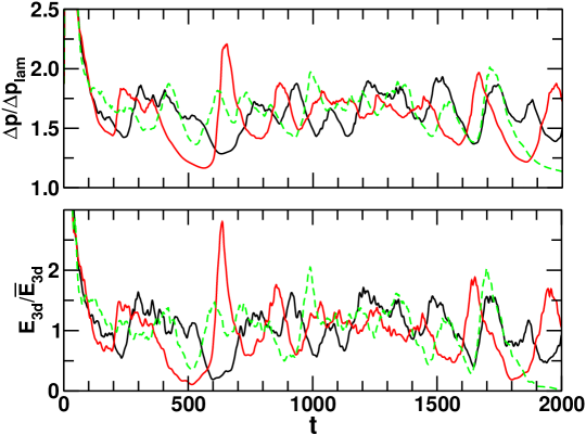
Figure 1: Traces of normalized pressure gradient (top) and energy content $E_{3d}$ (Eq. 3) (bottom) for three slightly different initial conditions at $Re=2100$. The initial energies are chosen high above the turbulent mean and the trajectories require about $200$ time units to relax to the neighborhood of the turbulent mean. Pressure drop and energy content show correlated fluctuations. Note that within statistical fluctuations the averages of the turbulent dynamics are the same. This includes the dashed trajectory which happens to decay near $t=2000$. The bottom frame shows the kinetic energy of the streamwise modulated part of the velocity field, $E_{3d}$, normalized by its turbulent mean as a measure of the velocity fluctuations

The measures that we apply to the turbulent runs are the pressure gradient required to maintain a constant mean flux and the energy variable $E_{3d}$, the kinetic energy in the streamwise modulated part of the velocity field,

$$E_{3d}=\sum_{n}\sum_{m\neq 0}\int_{0}^{R}|{\bf u}_{n,m}(r)|^{2}\,r\,dr\,.$$ (3)

The significance of $E_{3d}$ is that if it becomes too small, then the flow is too close to an axially translation invariant flow field and will eventually decay Zikanov (1996). We therefore terminate integration if it drops below a threshold of $10^{-4}$.

3 Turbulent lifetimes

Typical trajectories are shown in Fig. 1. Within about $150$ time units they relax towards the turbulent state. The dashed trace belongs to an initial condition for which the lifetime of the turbulent state is about $2000$: there is no indication of the decay until the energy $E_{3d}$ drops so low that turbulence cannot recover.

Scanning the lifetimes of turbulent states as a function of initial amplitude for different Reynolds number we obtain the results shown in Fig. 2. For sufficiently small amplitudes all states decay and the lifetimes are short. Beginning with a Reynolds number of $1800$ sharp peaks with very long lifetimes appear. Beyond $Re=2000$ several initial conditions reach lifetimes up to the integration cut-off of $t_{max}=2000$. Moreover, the variations in lifetimes between neighboring sampling points in amplitude increase.

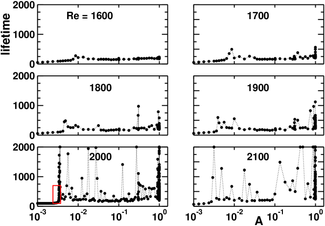
Figure 2: Turbulent lifetime vs. perturbation amplitude for different Reynolds numbers. For all Reynolds numbers a smooth region with short-lived states can be observed for small amplitudes. For larger Reynolds numbers this is followed by a ragged region of highly fluctuating lifetimes. The threshold amplitude that divides the two regions decreases with Reynolds number. The little rectangle at amplitudes of about $0.03$ at $Re=2000$ is further magnified in Fig. 3

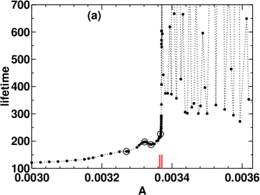
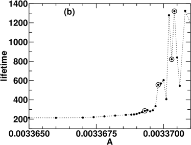
Figure 3: Successive magnifications of the lifetime variations with amplitude in the transition region for $Re=2000$. The left panel is a magnification of the box indicated in Fig. 2, the right one a magnification of the interval indicated in the left panel. Note the increased ordinate scale in the right panel.

The transition between the short lifetimes for the initial conditions that decay quickly towards the laminar state and the longer ones for trajectories that show some turbulent behaviour is a very rapid one. Successive magnifications of a small region in amplitude for $Re=2000$ are shown in Fig. 3. The increase is not monotonic, with modulations and structures superimposed.

Fig. 4 compares the energy traces for four initial conditions in two ranges of amplitude. Fig. 4a for the smaller mean amplitude shows that in an interval of width about $3\%$ of the mean amplitude the lifetimes increase by about $40\%$. At a slightly higher amplitude Fig. 4b shows that in an interval of relative width $3\cdot 10^{-4}$ the lifetimes increase by a factor of almost $4$!

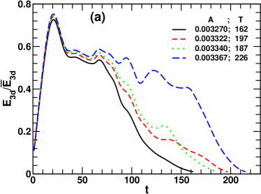
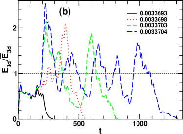
Figure 4: Energy traces for trajectories in small intervals of amplitude close to the transition region at $Re=2000$, marked by open circles in the corresponding panel in Fig. 3. The small differences in initial conditions are amplified and lead to noticeable differences in their evolution. For panel (b) the lifetimes are larger and the dynamics shows several large amplitude oscillations connected with the turbulent regeneration dynamics.

The strong fluctuations in lifetimes are not limited to variations with amplitude alone, they also occur when changing the Reynolds number for fixed amplitude, as shown in Fig. 5. Such fractal behaviour in the variations of lifetimes under parameter variation has previously been observed in plane Couette flow Schmiegel & Eckhardt (1997), Taylor-Couette flow for large radii Faisst & Eckhardt (2000); Eckhardt et al. (2002), and in models with a sufficient number of degrees of freedom Eckhardt & Mersmann (1999).

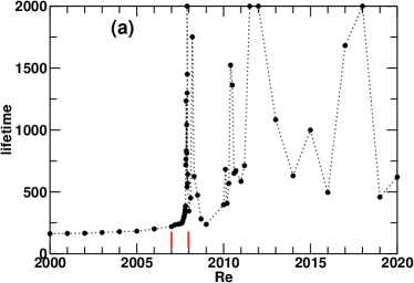
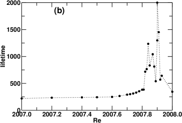
Figure 5: Variations of turbulent lifetimes with Reynolds number for a fixed initial disturbance amplitude $A=0.00327$. The parameter range marked in (a) by the shaded interval near $Re=2007$ is magnified in (b).

4 Lyapunov exponents

The sensitive dependence on variations of initial conditions can also be quantified in terms of Lyapunov exponents. For a trajectory ${\bf u}(t)$ and deviations $\delta{\bf u}(t)$ the largest Lyapunov exponent is defined as

$$\lambda=\lim_{||\delta u(0)||\rightarrow 0}\,\,\lim_{T\rightarrow\infty}\,\frac{1}{T}\log\frac{||\delta u(T)||}{||\delta u(0)||}\,,$$ (4)

where $||\cdot||$ denotes the Euclidian norm. Instead of a single $\lambda$ from an infinite time interval we calculate ensembles of finite-time Lyapunov exponents, extracted from the integration of a small deviation from the reference trajectory. The separation was measured after time intervals of $T=200$ units, and then rescaled to $||\delta u||=10^{-9}$. An initial time interval of $200$ units was omitted because of the transient relaxation of the initial conditions onto the turbulent state. Similarly, the last $200$ time units were omitted to avoid the decay to the laminar state. The infinite-time Lyapunov exponent was then approximated as the average of the finite-time Lyapunov exponents.

The instantaneous changes in the separation between neighbouring trajectories can be used to define local Lyapunov exponents Eckhardt & Yao (1993). They correlate strongly with large energy fluctuations, see Fig. 6a. When new large scale structures are generated the energy grows strongly and the Lyapunov exponent increases. Towards the end of a nonlinear regeneration cycle the energy goes down and the Lyapunov exponent decreases as well. Therefore, the fluctuations in the exponent are large and averages over at least $10^{4}$ time units are needed for the determination of reliable numbers. Obviously, this is very difficult to achieve for Reynolds numbers below $Re=2000$, where only very few trajectories stay turbulent for sufficiently long times.

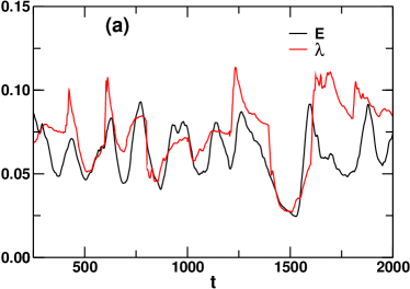
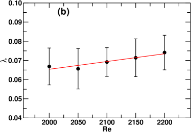
Figure 6: Lyapunov exponents in pipe flow. (a) Local Lyapunov exponent for a Reynolds number of $Re=2150$. The fluctuations in the local Lyapunov exponent correlate strongly with the energy content $E$ of the disturbance (in units of the energy of the laminar profile). (b) Largest Lyapunov exponent of the turbulent state with an error estimate based on the root mean square deviations of the ensemble of finite-time Lyapunov exponents. The line indicates a linear fit with slope $d\lambda/dRe\approx 4\times 10^{-5}$.

The largest Lyapunov exponent is shown in Fig. 6b. Its typical value is about $6.5\times 10^{-2}$ at Reynolds numbers around $2000$. For predictability this Lyapunov exponent implies that an uncertainty doubles after a time of $(\ln 2)/\lambda\approx 10$ units. Over a time interval of $200$ units a perturbation grows $10^{6}$-fold! Note that $200$ units is about the separation between two oscillations in the mean energy in Figs. 1 and 6a and is the typical duration of the regeneration cycle proposed in Hamilton et al. (1995); Waleffe (1995, 1997). Thus, the Lyapunov exponent is small in absolute value, but fairly large on the intrinsic time scales of the turbulent dynamics.

The extreme sensitivity of turbulent lifetimes to variations in initial conditions will make it next to impossible to prepare experimental perturbations sufficiently accurately to reproduce a run. A statistical analysis of, e.g., the distribution of lifetimes obtained by collecting data for several nearby initial conditions, should be more reliable. We therefore study $P(t)$, the probability that a flow started with some initial condition will still be turbulent after a time $t$. A related kind of statistics was proposed in Darbyshire & Mullin (1995): they analyzed the fraction $p$ of initial conditions that remained turbulent over the time $T$ it took for the perturbation to transit the distance between perturbation and detection. (Recall that we do not need to take this advection into account since our periodicity length is so short that the turbulence fills the entire volume.) In terms of our $P(t)$, this probability is $p=P(T)$. However, because of the unknown relation between the initial relaxation times in our simulations and the experiment we cannot compare values.

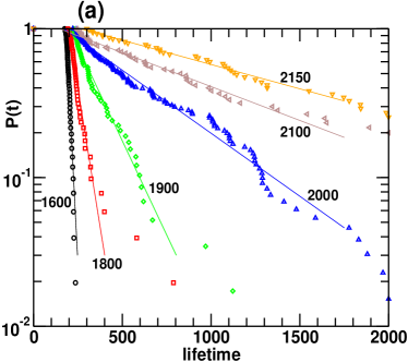
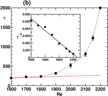
Figure 7: Turbulent lifetimes for different transitional Reynolds numbers. (a) Probability $P(t)$ for a single trajectory to still be turbulent after a time $t$ for six Reynolds numbers as indicated. Between $50$ and $100$ trajectories have been evaluated per Reynolds number. The distributions are well described by exponential distributions shown as straight lines. (b) Median $\tau$ of the turbulent lifetimes as a function of Reynolds number. The median and the fluctuations increase rapidly with Reynolds number until the median reaches the cut-off lifetime of $2000$ at $Re=2200$. The error bars indicate the statistical uncertainty of the median. The straight dashed line shows the linear increase in lifetime expected due to purely non-normal linear dynamics. The inset shows the inverse median lifetime vs. $Re$ and a linear fit, corresponding to a law $\tau(Re)\propto(Re_{c}-Re)^{-1}$, with $Re_{c}\approx 2250$.

For the lifetime statistics we used more than $50$ initial amplitudes each for eight Reynolds numbers in the range from $1600$ to $2200$. The amplitudes were fairly high, $\approx 1$, in order to assure transition to turbulence at least for a short time interval. The results for different Reynolds numbers are shown in Fig. 7.

The data support an exponential decay $P(t)\sim\exp(-\epsilon t)$ for large times, with $\epsilon$ the rate of escape from the turbulent state. An exponential distribution of turbulent lifetimes is a characteristic signature for escape from a chaotic saddle Kadanoff & Tang (1984); Tél (1991); Ott (1993). They have previously been seen in experiments Bottin & Chaté (1998); Bottin et al. (1998) and numerical studies on plane Couette flow Schmiegel (1999), as well as in Taylor-Couette flow Eckhardt et al. (2002). They seem to be a generic feature of the transition in shear flows that are not dominated by linear instabilities.

Another measure that can be extracted from the lifetime distributions is the median, $\tau=(\ln 2)/\epsilon$. The median is the time up to which half the states have decayed. It is also well suited for numerical studies since it is not affected by the cut-off in integration time. The median increases rapidly with Reynolds number as shown in Fig. 7b. Below $Re=1800$ the increase is mainly due to non-normal transient linear dynamics Grossmann (2000). When the Reynolds number is increased above $Re=2000$ the median of the turbulent lifetimes as well as the fluctuations rise rapidly until the median reaches the cut-off lifetime of $2000$ at $Re\approx 2200$. The inset in Fig. 7 shows the inverse median lifetime vs. $Re$ and among the possible fits for these data the most satisfactory ones supports a divergence like $(Re_{c}-Re)^{-1}$, with $Re_{c}\approx 2250$. Such a divergence would be connected with a transition from the chaotic saddle for lower $Re$ to an attractor for larger $Re$. However, it is known from other models that the lifetimes can increase rapidly without a true singularity Tél (1991); Crutchfield & Kaneko (1988). The question of whether we will arrive at a turbulent attractor cannot be answered here. But from the rapid increase it is clear that it will become an attractor for all practical purposes: for a setup with length $1000$ diameters the median will exceed this value for Reynolds number about $2130$. For this observation time the fraction of states with shorter lifetimes drops from $80\%$ of all initial conditions for $Re=2000$ to $40\%$ for $Re=2150$ and to zero for Re=$2200$. These numbers are obtained from the numerical simulations and include the initial transient; numbers in other simulations and experiments may be different, but the rapid increase will remain the same.

5 Conclusions

An exponential distribution of lifetimes can be obtained for a constant probability of decaying. In view of the internal dynamics and the characteristic times connected with it, one can interpret this as the probability of decaying towards the laminar state at the end of each turbulent regeneration cycle. The conclusion from the exponential distribution of lifetimes is that this probability remains constant during the evolution, independent of the ‘age’ of the trajectory.

It is worthwhile pointing out that the strong variation of the median lifetimes with $Re$ is not reflected in the Lyapunov exponent, which increases only linearly with $Re$: this shows that the chaotic dynamics on the turbulent saddle and the escape from it are two different processes with independent characteristics.

There are two predictions that should be accessible to experimental investigation: the behaviour near the boundary between laminar and turbulent and the exponential distribution of lifetimes. The increase in lifetime for increasing perturbation amplitude can be analyzed with a series of sensors along the pipe. The oscillations in Fig. 6a have a period of about $200$ time units, which translates into $200$ diameters. Thus, if a perturbation can be localized within a few radii, detectors that are further and further downstream might be able to reproduce some of the oscillations in Figure 4 as the perturbation amplitude is increased. Similarly, it might be possible to experimentally detect the Lyapunov exponents in the flow: with a Lyapunov exponent of about $0.07$, a $5\%$ uncertainty in the preparation of initial conditions will increase to $100\%$ in a time of about $40$ units, i.e. $40$ diameters. Thus, placing detectors at spacings of several diameters apart should allow a determination of the separation between flow states starting from similar initial conditions.

The second measurement is more easily performed: repeated runs with similar perturbations give the probability of finding a turbulent state that exists at least up to time $t$. The time can be varied again by placing detectors at different locations along the pipe. As explained, the exponential distribution of lifetimes is a property of the turbulent state in the transition region and will not depend critically on the type of initial conditions used. Exact reproduction of an initial condition is hence not essential here since all initial conditions relax to the same turbulent state. The median lifetime increases rapidly with Reynolds number, from about $220$ at $Re=1800$ to $750$ at $Re=2100$. Given the experimental limitations on the length of the pipe this region looks like a promising range for experiments. The mechanism studied here, the formation of a chaotic saddle, is fairly independent of the boundary conditions, but the quantitative characteristics may depend on it. Since the experiments will not have periodic boundary conditions in downstream direction and since the turbulence may be localized in puffs or slugs it will be interesting to see whether this will affect the lifetimes or its distribution.

A detailed analysis of the distribution of lifetimes is a task which is still much better suited for experiments than for numerics: it is not necessary to prepare the initial disturbance with highest precision, and the experimental observation time is of the order of $1$ minute for an experimental run, followed by about half an hour for the water to return to rest in the head-tank. On the other hand, a single trajectory in our computation takes up to $10$ days.

The picture that emerges from these data is that the transition to turbulence in pipe flow is connected with the formation of a chaotic saddle. The turbulent dynamics is chaotic, the lifetimes are exponentially distributed and the transition depends sensitively on the initial state. The same characteristics have been found in other shear flows without a linear instability as well Schmiegel & Eckhardt (1997); Eckhardt et al. (2002); Bottin et al. (1998); Faisst & Eckhardt (2000). The recent discovery of travelling waves in pipe flow for Reynolds numbers as low as $1250$ Faisst & Eckhardt (2003); Wedin & Kerswell (2003) strengthens this picture by providing some of the states around which the network of homoclinic and heteroclinic connections that carry the chaotic saddle may form.

Support by the German Science Foundation is greatfully acknowledged.

References

- Boberg & Brosa (1988) Boberg, L. & Brosa, U. 1988 Onset of Turbulence in a Pipe. Z. Naturforsch. 43a, 697–726.
- Bottin & Chaté (1998) Bottin, S. & Chaté, H. 1998 Statistical analysis of the transition to turbulence in plane Couette flow. Eur. Phys. J. B 6, 143–155.
- Bottin et al. (1998) Bottin, S., Daviaud, F., Manneville, P. & Dauchot, O. 1998 Discontinuous transition to spatiotemporal intermittency in plane Couette flow. Europhys. Lett. 43 (2), 171–176.
- Brosa (1989) Brosa, U. 1989 Turbulence without Strange Attractor. J. Stat. Phys. 55, 1303–1312.
- Canuto et al. (1988) Canuto, C., Hussaini, M., Quarteroni, A. & Zang, T. 1988 Spectral Methods in Fluid Dynamics. Springer-Verlag.
- Crutchfield & Kaneko (1988) Crutchfield, J. & Kaneko, K. 1988 Are attractors relevant to turbulence? Phys. Rev. Lett. 60, 2715–2718.
- Darbyshire & Mullin (1995) Darbyshire, A. & Mullin, T. 1995 Transition to turbulence in constant-mass-flux pipe flow. J. Fluid Mech. 289, 83–114.
- Eckhardt et al. (2002) Eckhardt, B., Faisst, H., Schmiegel, A. & Schumacher, J. 2002 Turbulence transition in shear flows. In Advances in turbulence IX (ed. I. Castro, P. Hancock & T. Thomas), p. 701. Barcelona: CINME.
- Eckhardt & Mersmann (1999) Eckhardt, B. & Mersmann, A. 1999 Transition to turbulence in a shear flow. Phys. Rev. E 60, 509–517.
- Eckhardt & Yao (1993) Eckhardt, B. & Yao, D. 1993 Local Lyapunov exponents. Physica D 65, 100–1008.
- Eggels et al. (1994) Eggels, J., Unger, F., Weiss, M., Westerweel, J., Adrian, R., Friedrich, R. & Nieuwstadt, F. 1994 Fully developed turbulent pipe flow: a comparison between direct numerical simulation and experiment. J. Fluid Mech. 268, 175–209.
- Faisst & Eckhardt (2000) Faisst, H. & Eckhardt, B. 2000 Transition from the Couette-Taylor system to the plane Couette system. Phys. Rev. E 61, 7227.
- Faisst & Eckhardt (2003) Faisst, H. & Eckhardt, B. 2003 Traveling waves in pipe flow. Phys. Rev. Lett. 91, 224502.
- Grossmann (2000) Grossmann, S. 2000 The onset of shear flow turbulence. Rev. Mod. Phys. 72, 603–618.
- Hamilton et al. (1995) Hamilton, J., Kim, J. & Waleffe, F. 1995 Regeneration mechanisms of near-wall turbulence structures. J. Fluid Mech. 287, 317–348.
- Hof et al. (2003) Hof, B., Juel, A. & Mullin, T. 2003 Scaling of the turbulence transition threshold in a pipe. Phys. Rev. Lett. 91, 244502.
- Kadanoff & Tang (1984) Kadanoff, L. & Tang, C. 1984 Escape from strange repellers. Proc. Natl. Acad. Sci. USA 81, 1276.
- Ma et al. (1999) Ma, B., van Doorne, C., Zhang, Z. & Nieuwstadt, F. 1999 On the spatial evolution of a wall-imposed periodic disturbance in pipe Poiseuille flow at . Part 1. Subcritical disturbance. J. Fluid Mech. 398, 181–224.
- Meseguer & Trefethen (2003) Meseguer, A. & Trefethen, L. 2003 Linearized pipe flow to Reynolds number . J. Comput. Phys. 186, 178–197.
- Ott (1993) Ott, E. 1993 Chaos in Dynamical Systems. Cambridge University Press.
- Priymak & Miyazaki (1998) Priymak, V. & Miyazaki, T. 1998 Accurate Navier-Stokes investigation of transitional and turbulent flows in a circular pipe. J. Comp. Phys. 142, 370–411.
- Quadrio & Sibilla (2000) Quadrio, M. & Sibilla, S. 2000 Numerical simulation of turbulent flow in a pipe oscillating around its axis. J. Fluid Mech. 424, 217–241.
- Reynolds (1883) Reynolds, O. 1883 An experimental investigation of the circumstances which determine whether the motion of water shall be direct or sinuous and the law of resistance in parallel channels. Phil. Trans. R. Soc. 174, 935–982.
- Rubin et al. (1980) Rubin, Y., Wygnanski, I. & Haritonidis, J. 1980 Further observations on transition in a pipe. In Laminar-Turbulent Transition (ed. R. Eppler & F. Hussein), pp. 19–26. Springer.
- Schmid & Henningson (1994) Schmid, P. & Henningson, D. 1994 Optimal energy density growth in Hagen-Poiseuille flow. J. Fluid Mech. 277, 197–225.
- Schmiegel (1999) Schmiegel, A. 1999 Transition to turbulence in linearly stable shear flows. PhD thesis, Philipps-Universität Marburg.
- Schmiegel & Eckhardt (1997) Schmiegel, A. & Eckhardt, B. 1997 Fractal stability border in plane Couette flow. Phys. Rev. Lett. 79 (26), 5250–5253.
- Schmiegel & Eckhardt (2000) Schmiegel, A. & Eckhardt, B. 2000 Persistent turbulence in annealed plane Couette flow. Europhys. Lett. 51, 395–400.
- Tél (1991) Tél, T. 1991 Transient chaos. In Directions in Chaos (ed. H. Bai-Lin, D. Feng & J. Yuan), , vol. 3. World Scientific, Singapore.
- Trefethen et al. (2000) Trefethen, L., Chapman, S., Henningson, D., Meseguer, A., Mullin, T. & Nieuwstadt, F. 2000 Threshold amplitudes for transition to turbulence in a pipe. http://xxx.uni-augsburg.de/abs/physics/0007092 .
- Trefethen et al. (1993) Trefethen, L., Trefethen, A., Reddy, S. & Driscol, T. 1993 Hydrodynamics stability without eigenvalues. Science 261, 578–584.
- Waleffe (1995) Waleffe, F. 1995 Transition in shear flows. Nonlinear normality versus non-normal linearity. Phys. Fluids 7, 3060–3066.
- Waleffe (1997) Waleffe, F. 1997 On a self-sustaining process in shear flows. Phys. Fluids 9, 883–900.
- Wedin & Kerswell (2003) Wedin, H. & Kerswell, R. 2003 Exact coherent structures in pipe flow: travelling wave solutions. submitted .
- Wygnanski & Champagne (1973) Wygnanski, I. & Champagne, F. 1973 On transition in a pipe. Part 1. The origin of puffs and slugs and the flow in a turbulent slug. J. Fluid Mech. 59, 281–335.
- Wygnanski et al. (1975) Wygnanski, I., Sokolov, M. & Friedman, D. 1975 On transition in a pipe. Part 2. The equilibrium puff. J. Fluid Mech. 69, 283–304.
- Zikanov (1996) Zikanov, O. 1996 On the instability of pipe Poiseuille flow. Phys. Fluids 8 (11), 2923–2932.