A theory of growth by differential sedimentation,
with application to snowflake formation

Abstract

A simple model of irreversible aggregation under differential sedimentation of particles in a fluid is presented. The structure of the aggregates produced by this process is found to feed back on the dynamics in such a way as to stabilise both the exponents controlling the growth rate, and the fractal dimension of the clusters produced at readily predictable values. The aggregation of ice crystals to form snowflakes is considered as a potential application of the model.

I Introduction

Simple models of cluster-cluster aggregation have been the focus of a great deal of interest, particularly over the last two decades. The structure of aggregates formed through a variety of dominating mechanisms (eg. diffusion limited meakin , reaction limited balletal and ballistic motion jullienandkolb ) have been studied through theoretical, experimental, and computational work.

Another aggregation mechanism which is relevant to several physical systems is that of differential sedimentation. Particles with a range of size and/or shape will almost inevitably sediment through a fluid at different speeds under the influence of gravity, leading to collisions. If there is some mechanism by which the particles stick on contact then aggregates will be formed. An example of this kind of phenomenon is the aggregation of ice crystals in Cirrus clouds. Small ‘pristine’ ice particles are formed at the top of the cloud, and proceed to fall through it, colliding with one another and sticking to produce aggregates (snowflakes).

The aim of this paper is to provide a simple model for growth by differential sedimentation which captures the essential physics of the system in the inertial flow regime, and to consider its application to snowflake formation. It is divided into five main parts - a description of the model and the assumptions underlying it; details of computer simulations and the results obtained from them; a theory section which offers an argument to account for the behaviour observed in the simulations; an investigation of the model’s applicability to snowflake formation; and a concluding discussion. The simulation results and their comparison to real cloud data have been presented briefly in a separate letter ourshortpreprint .

II Model

We focus on the dilute limit, where the mean free path between cluster-cluster collisions is large compared to the nearest neighbour distance between clusters. In this regime we can limit our interest to individual binary collision events, ignoring spatial correlation. As further simplifying approximations, we assume that clusters have random orientations which do not significantly change during a close encounter, that collsion trajectories are undeflected by hydrodynamic interaction, and that any cluster-cluster contacts result in a permanent and rigid junction.

In order to sample the collisions between clusters, we first formulate a rate of close approach. For any two clusters $i$, $j$ with nominal radii (see below) $r_{i}$ and $r_{j}$ respectively and fall speeds $v_{i}$ , $v_{j}$ , the frequency with which their centres pass closer than a distance $(r_{i}+r_{j})$ is proportional to the total area over which trajectories yielding a close approach event are possible, and the relative speed of the pair. This is illustrated in figure 1. The rate constant for approach closer than centre-to-centre separation $(r_{i}+r_{j})$ is therefore given by:

$$\Gamma_{ij}=\pi(r_{i}+r_{j})^{2}\left|v_{i}-v_{j}\right|.$$ (1)

In our computer simulations the nominal radii are chosen to fully enclose each cluster and the close approach rate calculated above is exploited to preselect candidate collision events. Collisions are accurately sampled by sequentially choosing pairs of clusters with probability proportional to $\Gamma_{ij}$, checking each pair for collision along one randomly sampled close approach trajectory, and correspondingly joining that cluster pair if they do indeed collide. In the theoretical arguments presented in section four, we make the simplifying assumption that all close approaches lead to collisions (or at least a fixed fraction of them do), using nominal radii based on fractal scaling from the cluster masses.

The model is completed by an explicit form for the fall speeds entering equation (1). We assume that the clusters are at most only partially penetrated by the fluid flow past them, so that cluster radius is the relevant length governing the drag force law. Then qualitatively and by dimensional argument we expect the same drag behaviour as for a falling sphere, which may be written in the form:

$$F_{d}=\rho\nu_{k}f(R_{e})$$ (2)

where $f$ is a function of the Reynolds number $R_{e}=rv/\nu_{k}$ alone, $\rho$ is the density of the surrounding fluid, and $\nu_{k}$ is the kinematic viscosity. Although details of the function $f(R_{e})$ should be different from spheres, we still expect to have inertial and Stokes regimes where $f$ takes the forms:

$$f(R_{e})\sim\left\{\begin{array}[]{c}R_{e}^{2}\text{ for inertial flow}\\ R_{e}\text{ for viscous flow}\end{array}\right\}\;.$$ (5)

We consider below the general form $f(R_{e})\sim R_{e}^{1/\alpha}$, with $\alpha$ as an adjustable parameter in order gain understanding spanning the two extreme regimes. Setting the drag force equal to the weight $mg$ of the cluster, the terminal velocity is then given by

$$v\sim\frac{\nu_{k}}{r}\left(\frac{mg}{\rho\nu_{k}^{2}}\right)^{\alpha}$$ (6)

where $\alpha=\frac{1}{2}$ for inertial flow and $\alpha\textrm{=1}$ for viscous flow. A more complete discussion of the fall speed is given by Mitchell mitchell96 , but provided $d_{f}\geq 2$ so that cluster projected area scales as the square of cluster radius, this reduces to a simple crossover between the above limits. The empirical crossover is very slow, spread over some three decades of Reynolds number, so fixed intermediate values of $\alpha$ can reasonably approximate behaviour over a significant range mitchell96 . In our simulations we took the radius determining the fall velocity to be proportional to the radius of gyration, and in our theoretical calculations we simply used the same nominal radii as for the collision cross sections above.

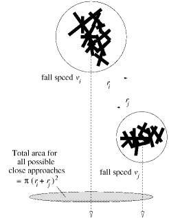
Figure 1: Illustration showing a possible scenario in which the centres of a pair of clusters falling at a relative speed $|v_{i}-v_{j}|$ come within a distance $(r_{i}+r_{j})$ of one another (a close approach). The shaded circle illustrates the total area encompassing all possible close approach trajectories $=\pi(r_{i}+r_{j})^{2}$.

III Computer simulations and results

The primary particles used at the beginning of the simulations were rods of zero thickness, half of which had a length (and mass) of unity, and half of which were twice as long and massive. Purely monodisperse initial conditions are not possible in this model, since $|v_{i}-v_{j}|$ would be zero. Apart from this special case however, it is anticipated that the asymptotic behaviour of the system should be insensitive to the initial distribution, and indeed the results described in this section appear to be preserved for a variety of starting conditions.

In aggregation models it is typically the case (eg. Vicsek and Family vicsekandfamily ) that after the distribution has had time to ‘forget’ its initial conditions it will approach a universal shape. This is usually expressed by the ‘dynamical scaling’ ansatz, which states that as $m,s\rightarrow\infty$:

$$n_{m}(t)=s(t)^{-2}\phi\left[\frac{m}{s(t)}\right]$$ (7)

where $n_{m}(t)$ is the number of clusters of mass $m$ at time $t$, and the rescaled distribution $\phi$ is a function of $x=m/s(t)$ alone. The quantity $s(t)$ is a characteristic cluster mass, and for non-gelling systems one expects that a suitable choice is given by the weight average cluster mass, $s(t)=\sum_{i}m_{i}^{2}/\sum_{i}m_{i}$. Using this choice our simulation data conform well to scaling, as shown in the left panel of figure 2.

The shape of the rescaled distribution was studied. A plot of $\int_{x}^{\infty}\phi(x^{\prime})\text{d}x^{\prime}$ as a function of $x$ is shown in the right panel of figure 2 and shows an exponential decay for very large $x$, with a ‘super-exponential’ behaviour taking over as $x$ approaches unity from above. This behaviour appears to be universal for all values of $\alpha$ in the range studied.

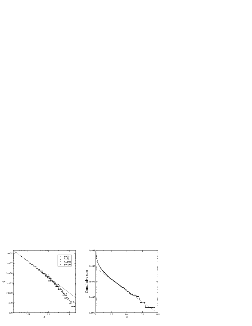
Figure 2: Scaling of the cluster mass distribution. The left panel shows how the rescaled cluster size distribution $\phi=s(t)^{2}n_{m}(t)$ converges to a universal function of rescaled cluster size $x=m/s(t)$, where the data are overlayed for different values of the weight average cluster size, $s(t)=20,50,150,400$. The scales are logarithmic and a least squared fit $\phi(x)\sim x^{-1.6}$ for $x\leq 10^{-2}$ is shown by the dashed line. In the right hand panel $\int_{x}^{\infty}\phi(x^{\prime})\text{d}x^{\prime}$ is shown on a semi-log plot, illustrating the exponential tail (dashed line is intended to guide the eye). Both simulations began with 250,000 rods, and used $\alpha=0.55$ in the sedimentation law.

For $x\ll 1$ the qualitative form of $\phi(x)$ was found to fall into two distinct catagories depending on the value of $\alpha$. For $\alpha\geq\frac{1}{2}$ the distribution appears to diverge as a power law: $\phi(x\rightarrow 0)\sim x^{-\tau}$, as shown in figure 2 for $\alpha=0.55$. The exponent $\tau$ was found to be approximately constant at $\tau\simeq 1.6\pm 0.1$ over the range $\frac{1}{2}\leq\alpha\leq\frac{2}{3}$. For $\alpha<\frac{1}{2}$ the distribution was found to be peaked, with a maximum at some small size $x_{m}$, followed by a power law decay for $x_{m}\ll x\ll 1$.

Comparison with other aggregation models suggests that the clusters produced are likely to be fractal in their geometry, and in particular cluster mass and (average) radius should be in a power law relationship $m\sim r^{d_{f}}$ where $d_{f}$ is the fractal dimension. A log plot of radius of gyration against mass for all the clusters produced over the course of the simulation is shown in figure 3. Also shown in this figure is the logarithmic derivative of the above plot, which shows the variation in the apparent fractal dimension of the clusters with size. From this plot, it seems that the fractal dimension approaches an asymptotic value as $m\rightarrow\infty$; in the case shown ($\alpha=0.55$) we estimate this value as $d_{f}\simeq 2.2\pm 0.1$. The value of this limiting fractal dimension was found to vary with $\alpha$ as shown in figure 4. Note that our assumption $d_{f}\geq 2$, required to support the assumed fall speed relationship, is indeed satisfied for the physical range $\alpha\geq 1/2$.

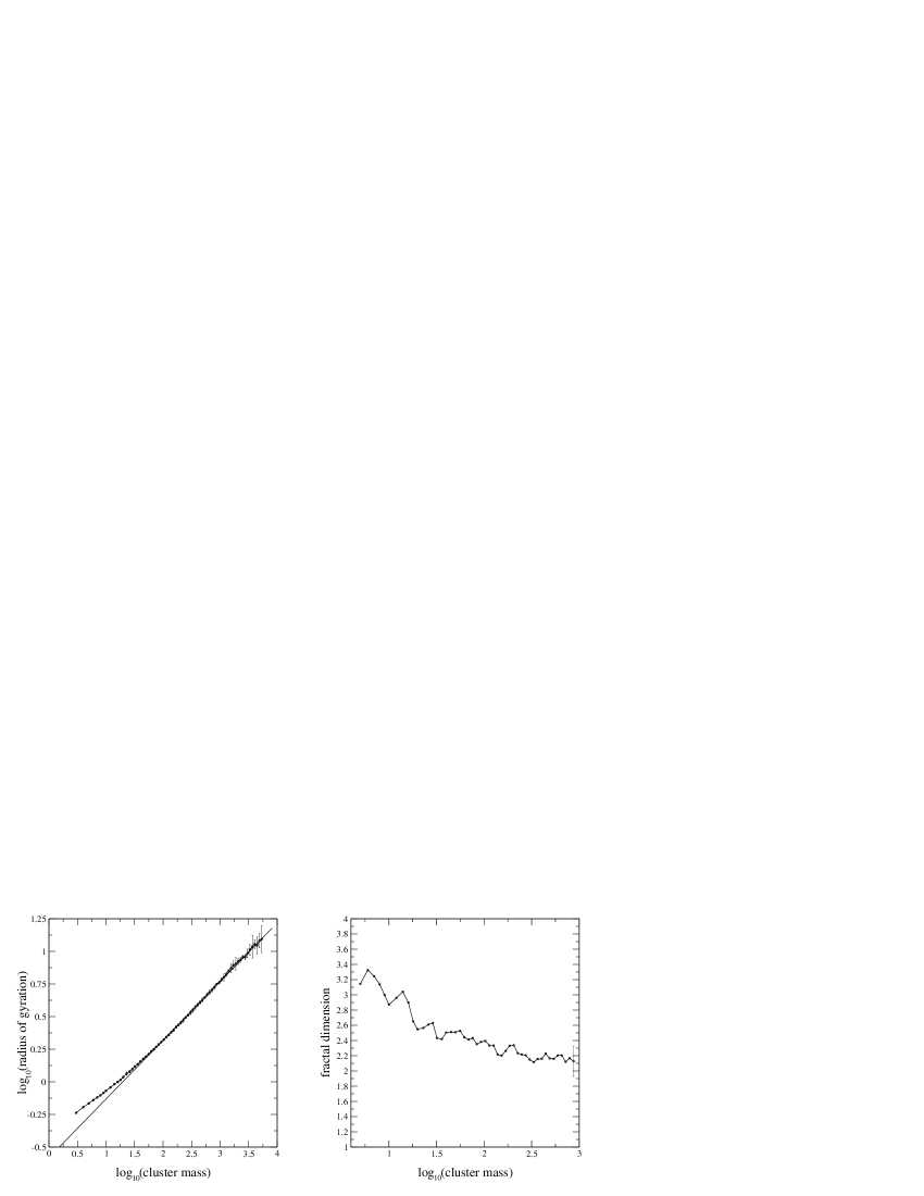
Figure 3: Left hand panel shows a log plot of radius of gyration as a function of cluster mass for $\alpha=0.55$, averaged over four runs of 250,000 initial rods. Solid line indicates the theoretical prediction for the fractal dimension. The right hand panel shows the inferred fractal dimension as a function of cluster mass. Error bars are one standard deviation. Data points with $\sigma>0.3$ have not been plotted.

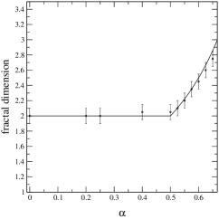
Figure 4: Variation of the fractal dimension as a function of the parameter $\alpha$. Circles are simulation data, solid line indicates theoretical prediction.

IV Theory

The most common theory used to describe cluster-cluster aggregation problems is that of von Smoluchowksi smoluchowski , which provides a set of mean-field rate equations for the evolution of the cluster mass distribution:

$$\frac{\text{d}n_{k}(t)}{\text{d}t}=\frac{1}{2}\sum_{i+j=k}K_{ij}n_{i}(t)n_{j}(t)-n_{k}(t)\sum_{j=1}^{\infty}K_{ij}n_{j}(t).$$ (8)

where $n_{k}(t)$ is the number of clusters of mass $k$ at time $t$ (per unit volume). The kernel $K_{ij}$ contains the physics of the problem, being a symmetric matrix, the elements of which govern the rate of aggregation between pairs of clusters expressed (only) in terms of their masses $i$ and $j$. Analytical solutions of Smoluchowski’s equations have not been obtained except for a few special cases of $K_{ij}$. However, Van Dongen and Ernst vdande85 have shown that for non-gelling kernels (see below) the solutions approach the dynamical scaling form of equation (7) in the large-mass, large-time limit; substituting this into equations (8) allows one to obtain some information about the asymptotic behaviour of the rescaled cluster size distribution $\phi(x)$.

To apply this theory we need to compute the reaction rates $K_{ij}$ , which means averaging collision rate with respect to cluster geometry at fixed masses. This we estimate by substituting averages from fractal scaling for the radii in equations (1) for the close approach rate and (6) for the fall speeds, and assuming constant collision efficiency leading to:

$$K_{ij}\sim\left|i^{\alpha-1/d_{f}}-j^{\alpha-1/d_{f}}\right|\left(i^{1/d_{f}}+j^{1/d_{f}}\right)^{2}.$$ (9)

Van Dongen and Ernst’s analysis is sensitive to two exponents characterising the scaling of the coagulation kernel in the limit $1\ll i\ll j$,

$$K_{ij}\sim i^{\mu}j^{\nu}$$ (10)

which in our case yields:

$$\mu = \min(0,\alpha-d_{f}^{-1})$$ (11)

$$\nu = \max(\alpha+d_{f}^{-1},2d_{f}^{-1}).$$ (12)

A third exponent combination $\lambda=\mu+\nu=\alpha+d_{f}^{-1}$ controls the growth of the average cluster mass through the differential equation $\dot{s}(t)=ws(t)^{\lambda}$, where $w$ is a constant, and for the non-gelling case we require $\lambda\leq 1$.

Our identification of the exponent $\nu$ is crucial to a mechanism by which the fractal dimension can control the dynamics. If the fractal dimension is low enough, then the exponent $\nu$ will exceed unity. However, Van Dongen vandongen has shown that the Smoluchowski equations predict the formation of an infinite cluster instantly in such a situation. In a finite system this clearly cannot occur, and it simply means that a few clusters will quickly become much larger than the others with their growth dominated by accretion of small ones. In this scenario the growth of the large clusters approaches that of ballistic particle-cluster aggregation, where it has been shown by Ball and Witten ballandwitten that the fractal dimension of the clusters produced tends to $d_{f}=3$. This increased fractal dimension reduces the value of $\nu$, forcing it back to a value of one if $\alpha\leq\frac{2}{3}$. Through this feedback mechanism, a bound is placed on the fractal dimension $d_{f}\geq\max[2,(1-\alpha)^{-1}]$ for $\alpha\leq\frac{2}{3}$.

The system could perhaps settle in a state where $\nu<1$. However, the growth in such a regime is much less biased towards collisions between clusters of disparate sizes, and the distribution is relatively monodisperse. This would tend to make collisions between clusters of a similar size likely, leading to much more open structures, with a lower fractal dimension, in turn acting as a feedback mechanism to increase the value of $\nu$. The authors suggest that, at least over some range of $\alpha$, this effect will force the system towards the $\nu=1$ state. The discontinuity in the polydispersity of the system at $\nu=1$ forces the system to organise itself such that it can remain at that point. This is similar to the argument put forward by Ball et al balletal for reaction limited aggregation.

If it is accepted that $\nu\rightarrow 1$ then the fractal dimension of the clusters produced ought to be directly predictable from equation (12) :

$$d_{f}=\max[2,(1-\alpha)^{-1}],\quad\alpha\leq\frac{2}{3}.$$ (13)

A curve showing this theoretical behaviour is superimposed on the simulation data in figure 4, and appears to show good agreement up to $\alpha\simeq\frac{2}{3}$. For $\alpha>\frac{2}{3}$ the theoretical prediction is that $d_{f}=3$ and $\nu=\alpha+\frac{1}{3}>1$, but because of its somewhat pathological nature we have not attempted to make simulations in this regime. It is however clear from the extrapolation of our results in figure 4 that this is likely to hold.

Obtaining an exact form for the cluster size distribution $\phi(x)$ is a non-trivial exercise. However, following the methodology of Van Dongen and Ernst vdande85 , we consider the small-$x$ behaviour of $\phi(x)$ when $d_{f}<\alpha^{-1}$ (ie. $\mu<0$). In such a regime the small-$x$ behaviour is dominated by collisions between clusters of disparate sizes; the gain term in the Smoluchowski equations may therefore be neglected, and one attempts to solve the integro-differential equation: $w[x\phi^{\prime}(x)+2\phi(x)]=\phi(x)\int_{0}^{\infty}K(x,y)\phi(y)\text{d}y$. For $x\ll y$, the kernel (9) may be approximated to $K(x,y)\simeq x^{\mu}y^{\nu}-y^{\lambda}$, and one obtains:

$$\phi(x)=x^{-\tau}\exp\left[\frac{x^{\mu}p_{\nu}}{w\mu}\right]$$ (14)

where $p_{i}$ is the $i^{th}$ moment of the rescaled distribution $\phi(x)$, and the exponent $\tau$ is given by $\tau=2+p_{\lambda}w^{-1}$. It is clear that $\lim_{x\rightarrow 0}[\phi(x)]=0$. As $x$ increases from zero, $\phi(x)$ also increases, until reaching a maximum at $x_{m}=({w\tau}/{p_{\nu}})^{1/{\mu}}$. For $x_{m}\ll x\ll 1$ the distribution has an approximately algebraic decay $\phi(x)\sim x^{-\tau}$. This ‘bell-shaped’ curve is consistent with the behaviour seen in the computer simulations when $\alpha<\frac{1}{2}$.

In the case $d_{f}>\alpha^{-1}$, it has been shown vdande85 that for all kernels with $\mu=0$, $\nu\leq 1$ the cluster size distribution diverges as $x\rightarrow 0$ with the form

$$\phi(x)\sim x^{-\tau}$$ (15)

where $\tau=2-p_{\lambda}w^{-1}$. This behaviour is consistent with the simulation for $\alpha\geq\frac{1}{2}$. The change in the qualitative shape of $\phi(x\ll 1)$ around $\alpha=\frac{1}{2}$ then is further evidence to suggest that the system selects to sit at $\nu=1$.

The shape of $\phi(x\gg 1)$ has also been studied by Van Dongen and Ernst vdande87 . They have shown that for non-gelling kernels, the tail of the distribution is expected to take the form

$$\phi(x)\sim x^{-\theta}\text{e}^{-\delta x}$$ (16)

where $\theta$ and $\delta$ are constants. This would appear to be consistent with the behaviour observed in the simulations for all values of $\alpha$, providing an exponentially dominated cut-off at large $x$.

V Application to snowflake formation

The principle motivation for the model presented in this paper was to attempt to understand some of the properties of Cirrus clouds. These are high altitude clouds with a base betwen 5,500 and 14,000 metres and they are usually composed solely of ice crystals PandKlett . Amongst others, Heymsfield and Platt heymandplatt have observed that the ice crystals in these clouds are predominantly composed of columns, bullets, bullet-rosettes and aggregates of these crystal types. It is these aggregates which we hope to model, since the dominant mechanism by which they grow is believed to be through differential sedimentation (eg. Field and Heymsfield field ). We therefore ignore the effects of diffusional growth, turbulence, mixing, and particle breakup, in order to concentrate on the effects of this mechanism alone. The Reynolds number for aggregates of a few crystals is typically between $\simeq 10$—$100$ which ought to be modelled acceptably by our inertial flow approximation. Because we have not modelled the detailed hydrodynamics we may also be ignoring subtleties such as wake capture.

All of the results below are presented for the purely inertial regime (assumed to be the most relevant to this problem) where $\alpha=\frac{1}{2}$. The initial particles were rods of zero thickness - however, the asymptotic behaviour is anticipated to be insensitive to the initial conditions, and indeed by running the simulation with ‘bullet rosettes’ for the initial particles (three rods, crossing one another at right angles, through a common centre), no change in the end results were found, only in the approach to scaling.

Ice crystal aggregates have been studied through the use of cloud particle imagers during aircraft flights through ice clouds. Sample images from such a flight are shown in figure 5, alongside some of our simulation clusters. Using this experimental data, the geometry and size distribution of ice particles in these clouds has been studied, allowing for quantitative comparison between theory and experiment.

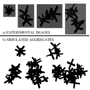
Figure 5: Projected images of a) ice crystal aggregates obtained using a cloud particle imager (CPI, SPEC Inc., USA) during an aircraft flight through a Cirrus cloud at temperatures between $-44^{\circ}$C to $-47^{\circ}$C, and b) sample clusters from our simulations.

The fractal dimension of snowflakes in Cirrus may be inferred from the work of Heymsfield et al heyma . By measuring the effective density $\rho_{e}$ of bullet and bullet-rosette aggregates as a function of their maximum linear dimension $D$, and fitting a power law to their data, they found the relationship $\rho_{e}\sim D^{-0.96}$. This scaling implies that the aggregates have a fractal dimension of $d_{f}=2.04$, which is consistent with the values predicted by our model (simulation giving $d_{f}=2.05\pm 0.1$ and theory giving $d_{f}=2$).

The aspect ratio of the clusters may also be calculated. Random projections of simulation clusters were taken. The maximum dimension of the projection $D$ was measured, as was the maximum dimension in the direction perpendicular to that longest axis, $D_{w}$. The ratio of these two spans were binned by maximum dimension, averaged, and plotted as a function of $D$ as shown in figure 6. The ratio quickly approaches an asymptotic value of approximately $0.65\pm 0.05$. This compares well to the measurements of Korolev and Isaac korolevandisaac , where the ratio seems to approach a value of $\simeq 0.6-0.7$.

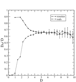
Figure 6: Aspect ratio of simulation clusters as a function of their maximum dimension. The curve seems to approach an asymptotic value of $\simeq 0.65$, independent of the initial conditions used: here we show data for both rods and rosettes.

Finally, the shape of the snowflake distribution of linear size may also be compared with experiment. Field and Heymsfield field presented particle size distributions of the maximum length $D$ of ice particles in a Cirrus cloud. The data were obtained with an aircraft and represent in-cloud averages of particle size distributions (number per unit volume per particle size bin width) along 15km flight tracks ranging from an altitude of 9500m ($-50^{\circ}$C) to 6600m ($-28^{\circ}$C). To compare this data to the distributions obtained from simulation, we first normalise the data, and then make use of the dynamical scaling form (7), to collapse the distributions onto a single curve. Details of this are given in the appendix to this paper. The resulting histograms are shown in figure 7 and appear to show quite good agreement, given the level of approximation present in our model.

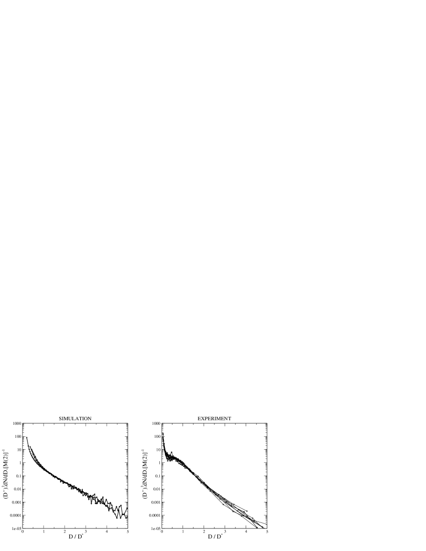
Figure 7: The left hand panel shows the distribution of clusters by linear size at various stages of the simulation, rescaled in such a way as to collapse the data (see appendix). Initial conditions were 250,000 rods and the parameter $\alpha$ was set to a value of $\frac{1}{2}$. The right hand panel is a test of the same scaling using the experimental data presented by Field and Heymsfield field .

VI Discussion and conclusions

A simple mean-field model of aggregation by differential sedimentation of particles in an inertial flow regime has been constructed, simulated by computer, and analysed theoretically in terms of the Smoluchowski equations. It has been shown that there is strong numerical evidence, in addition to a theoretical argument, to back up the idea that the polydispersity of the distribution and the fractal dimension feed back on one another in such a way as to stabilise the system at $\nu=1$. Above this value, the dominance of collisions between clusters of very different sizes is so great as to push $d_{f}$ towards a value of three. This in turn pulls the exponent $\nu$ back down to unity. For $\nu<1$ the system is quite monodisperse, resulting in relatively many collisions between clusters of similar sizes, and the fractal dimension is reduced, forcing $\nu$ back up. The discontinuity in the shape of the distribution around $\nu=1$ is thought to provide the mechanism by which the system can stabilise at that point.

If it is accepted that $\nu\rightarrow 1$, then the fractal dimension of the clusters produced may be predicted, and figure 4 shows that this prediction agrees well with simulation results for $0\leq\alpha\leq\frac{2}{3}$. The sudden change in the behaviour of $d_{f}(\alpha)$ and in the small-$x$ form of the cluster size distribution around $\alpha=\frac{1}{2}$ is strong evidence for the self-organisation proposed between $d_{f}$ and $\nu$.

For $\alpha>\frac{2}{3}$ the system is forced into a regime where $\nu>1$, which has been regarded as unphysical because the Smoluchowski equation (8) predicts infinite clusters in zero time vandongen . In the light of our results this regime merits further study beyond the Smoluchowski equation approximation workinprogress . The value $\alpha=1$ is given by viscous flow, but here our form for $\Gamma_{ij}$ does not include all of the relevant physics: in particular, small clusters may be caught in the fluid flow, and swept around larger clusters rather than hitting them, reducing the dominance of big-little collisions. This has been discussed in more detail for the particle-cluster aggregation case by Warren et al warrenetal .

The application of the model to the formation of ice crystal aggregates in Cirrus clouds has been considered: the fractal dimension, aspect ratio, and shape of the cluster size distribution seen in the model were all found to be consistent with experimental data. This is a promising indication that the ideas presented in this paper may be an acceptable model for the essential physics of snowflake aggregation in Cirrus.

*

Appendix A Scaling of the cluster radius distribution

Experiments have reported the distribution of ice aggregates by linear span rather than by mass, and we present here how that distribution $\frac{\text{d}N}{\text{d}D}$ should naturally be rescaled. This tests the dynamical scaling ansatz which, for the mass distribution, gave $\frac{\text{d}N}{\text{d}m}=n_{m}=s^{-a}\phi(m/s)$, where $a=2$ in mass-conserving systems. We anticipate fractal scaling so that $m\sim D^{d_{f}}$ and hence:

$$\frac{\text{d}N}{\text{d}D}\sim D^{d_{f}-1}s^{-a}\phi\left(\frac{m}{s}\right).$$ (17)

From this expression we may calculate the moments of the distribution $M(b)\equiv\int\frac{\text{d}N}{\text{d}D}D^{b}\text{d}D$ in terms of the average cluster mass $s(t)$:

$$M(b)\sim s^{-a+1+b/d_{f}}\int_{1/s}^{\infty}x^{b/d_{f}}\phi(x)\text{d}x$$ (18)

where $x=m/s$. At small sizes we expect $\phi(x)\sim x^{-\tau}$. If $b>d_{f}(\tau-1)$ therefore, the integral converges as $s\rightarrow\infty$, and $M(b)\sim s^{-a+1+b/d_{f}}$. From our simulations, we have measured $\tau\simeq 1.6$, $d_{f}\simeq 2$, and so the lowest integer moment which scales in this way is the second. We therefore choose this to normalise our data:

$$[M(2)]^{-1}\frac{\text{d}N}{\text{d}D}\sim D^{d_{f}-1}s^{-1-2/d_{f}}\phi\left(\frac{m}{s}\right)$$ (19)

which, defining the average cluster diameter $D^{*}\equiv M(3)/M(2)\sim s^{1/d_{f}}$ yields:

$$[M(2)]^{-1}\frac{\text{d}N}{\text{d}D}\sim(D^{*})^{-3}\psi\left(\frac{D}{D^{*}}\right),$$ (20)

where $\psi(y)=y^{d_{f}-1}\phi(y^{d_{f}})$. Hence, if we assume that $d_{f}$ approaches a constant value, plots of $\{[M(2)]^{-1}.\frac{\text{d}N}{\text{d}D}.(D^{*})^{3}\}$ against $(D/D^{*})$ should all lie on a single curve.

References

- (1) C.D. Westbrook, R.C. Ball, P.R. Field and A.J. Heymsfield, arXiv:physics/0310164 (2003)
- (2) P. Meakin, Phys. Rev. Lett 51, 1119 (1983)
- (3) R.C. Ball et al, Phys. Rev. Lett. 58, 274 (1987)
- (4) R. Jullien and M. Kolb, J. Phys. A 17, L639 (1984)
- (5) D.L. Mitchell, J. Atmos. Sci. 53 1710 (1996)
- (6) T. Vicsek and F. Family, Phys. Rev. Lett. 52 1669 (1984)
- (7) M. von Smoluchowksi, Phys. Z. 17 585 (1916)
- (8) P.G.J. Van Dongen and M.H. Ernst, Phys. Rev. Lett. 54, 1396 (1985)
- (9) P.G.J. Van Dongen, J. Phys. A 20, 1889 (1987)
- (10) R.C. Ball and T.A. Witten, Phys. Rev. A 29, 2966 (1984)
- (11) P.G.J. Van Dongen and M.H. Ernst Physica A 145, 15 (1987)
- (12) H.R. Prupappacher and J.D. Klett, ”Microphysics of clouds and precipitation”, 2nd ed., Kluwer, London (1997).
- (13) A.J. Heymsfield and R. Platt, J. Atmos. Sci. 41, 846 (1984)
- (14) P.R. Field and A.J. Heymsfield, J. Atmos. Sci. 60, 544 (2003)
- (15) A.J. Heymsfield et al, J. Atmos. Sci. 59, 3 (2002)
- (16) A. Korolev and G. Isaac, J. Atmos. Sci. 60, 1795 (2003)
- (17) R.C. Ball and C.D. Westbrook - work in progress
- (18) PB Warren, RC Ball and A Boelle, Europhys. Lett. 29 339-344 (1995).