Large-scale grid-enabled lattice-Boltzmann simulations of complex fluid flow in porous media and under shear

Abstract

Lattice-Boltzmann, porous media, complex fluids under shear,
grid computing, computational steering Well designed lattice-Boltzmann codes exploit the essentially embarrassingly parallel features of the algorithm and so can be run with considerable efficiency on modern supercomputers. Such scalable codes permit us to simulate the behaviour of increasingly large quantities of complex condensed matter systems. In the present paper, we present some preliminary results on the large scale three-dimensional lattice-Boltzmann simulation of binary immiscible fluid flows through a porous medium derived from digitised x-ray microtomographic data of Bentheimer sandstone, and from the study of the same fluids under shear. Simulations on such scales can benefit considerably from the use of computational steering and we describe our implementation of steering within the lattice-Boltzmann code, called LB3D, making use of the RealityGrid steering library. Our large scale simulations benefit from the new concept of capability computing, designed to prioritise the execution of big jobs on major supercomputing resources. The advent of persistent computational grids promises to provide an optimal environment in which to deploy these mesoscale simulation methods, which can exploit the distributed nature of compute, visualisation and storage resources to reach scientific results rapidly; we discuss our work on the grid-enablement of lattice-Boltzmann methods in this context.

1 Introduction

The length and time scales that can be modelled using microscopic modelling techniques such as molecular dynamics are circumscribed by the limited computational resources available today. Even with today’s fastest computers, the accessible length scales are on the order of nanometres and the time scales restricted to the nanosecond range. Mesoscopic models open the way to studies of time dependent, non-equilibrium phenomena occurring in much larger systems and on orders of magnitude longer timescales, thus bridging scales between microscopic models and macroscopic or continuum approaches.

In this paper, we use the lattice-Boltzmann method to model binary fluids under shear and flow in a porous medium. In the porous medium case, we are now able to reach length scales for the simulated fluid flow which can be compared directly to data gleaned from magnetic resonance imaging experiments. In the case of fluids under shear, one must take care of finite size effects which make it undesirable to study cubic systems, but rather preferable to study systems of high aspect ratio. In this paper we present preliminary results, but expect to return with extensive descriptions of the two applications in the near future. Both problems are very computationally demanding and require today’s top-of-the-range supercomputers and large scale data storage facilities. Since these resources are expensive, we have to handle them with care and minimize wastage of CPU time and disk space. A good initial position is to make sure that our simulations do not last longer than needed and do not produce more data than necessary. But more than this, computational steering allows us to interact with a running simulation and adjust simulation parameters and data dumping rates; it also enables us to monitor the state of our simulations and react immediately if they do not behave as expected, as we shall discuss later. The world wide effort to develop reliable computational grids gives us hope to run our simulations in an even more efficient way. Computational grids are a collection of geographically distributed and dynamically varying resources, each providing services such as compute cycles, visualization, storage, or even experimental facilities. It is hoped that computational grids will offer for information technology what electricity grids offer for other aspects of our daily life: a transparent and reliable resource that is easy to use and conforms to commonly agreed standards [Foster and Kesselman, 1999a, Berman et al., 2003]. Then we shall be able to use the available compute resources in a transparent way, leaving to smart middleware the task of finding the best available machines to run simulations on and migrate them to other platforms if necessary to ensure optimal performance. Grids will also allow storage, compute and visualization resources to be widely distributed without our having to care about their location.

The main purpose of the present paper is to introduce the concepts of computational steering and grid computing to an audience of computational scientists, concerned here with simulation of fluid dynamics. The paper is structured as follows. After a short introduction to our lattice-Boltzmann method in Section 2, we give a description of our implementation of computational steering in Section 3 and explain the advantages we expect to gain from the advent of computational grids in Section 4. Sections 5 and 6 contain our preliminary results on large scale grid-enabled simulations of fluids under shear and in porous media. We present our conclusions in Section 7.

2 A lattice-Boltzmann model of immiscible fluids

During the last decade, many authors have shown that the lattice-Boltzmann algorithm is a powerful method for simulating fluid dynamics. This success is due to its simplicity and to facile computational implementations [Chin et al., 2003, Love et al., 2003, Nekovee et al., 2001, Succi, 2001]. Instead of tracking individual atoms or molecules, the lattice-Boltzmann method describes the dynamics of the single-particle distribution function of mesoscopic fluid packets.

In a continuum description, the single-particle distribution function $f_{1}({{\bf r}},{{\bf v}},t)$ represents the density of fluid particles with position ${{\bf r}}$ and velocity ${{\bf v}}$ at time $t$, such that the density and velocity of the macroscopically observable fluid are given by $\rho({{\bf r}},t)=\int f_{1}({{\bf r}},{{\bf v}},t){\mathrm{d}}{{\bf v}}$ and ${{\bf u}}({{\bf r}},t)=\int f_{1}({{\bf r}},{{\bf v}},t){{\bf v}}{\mathrm{d}}{{\bf v}}$ respectively. In the non-interacting, long mean free path limit, with no externally applied forces, the evolution of this function is described by the Boltzmann equation

$$\left(\partial_{t}+{{\bf v}}\cdot{{\bf\nabla}}\right)f_{1}=\Omega[f_{1}].$$ (1)

While the left hand side describes changes in the distribution function due to free particle motion, the right hand side models pairwise collisions. This collision operator $\Omega$ is an integral expression that is often simplified [Bhatnagar et al., 1954] to the linear Bhatnagar-Gross-Krook (BGK) form

$$\Omega[f]\simeq-\frac{1}{\tau}\left[f-f^{\mathrm{(eq)}}\right].$$ (2)

This collision operator describes the relaxation, at a rate controlled by a characteristic time $\tau$, towards a local Maxwell-Boltzmann equilibrium distribution $f^{\mathrm{(eq)}}$. It can be shown that distributions governed by the simple Boltzmann-BGK equation conserve mass, momentum, and energy [Succi, 2001]. They obey a non-equilibrium form of the second law of thermodynamics [Liboff, 1990] and the Navier-Stokes equations for macroscopic fluid flow are obeyed on coarse length and time scales  [Chapman and Cowling, 1952, Liboff, 1990].

By discretizing the single-particle distribution function in space and time, one obtains the usual lattice-Boltzmann formulation, where the positions ${{\bf r}}$ on which $f_{1}({{\bf r}},{{\bf v}},t)$ is defined are restricted to points ${{\bf r}}_{i}$ on a Bravais lattice. The velocities ${{\bf v}}$ are restricted to a set ${{{\bf c}}_{i}}$ joining points on the lattice and the density of particles at lattice site ${{\bf r}}$ travelling with velocity ${{{\bf c}}_{i}}$, at timestep $t$ is given by $f_{i}({{\bf r}},t)=f({{\bf r}},{{{\bf c}}_{i}},t)$. The fluid’s density and velocity are given by

$$\rho({{\bf r}})=\sum_{i}f_{i}({{\bf r}})$$ (3)

$${{\bf u}}({{\bf r}})=\sum_{i}f_{i}({{\bf r}}){{{\bf c}}_{i}}$$ (4)

The discretized Boltzmann description can be evolved as a two-step procedure. In the collision step, particles at each lattice site are redistributed across the velocity vectors; this process corresponds to the action of the collision operator. In the advection step, values of the post-collisional distribution function are propagated to adjacent lattice sites.

By combining the two steps, one obtains the lattice-Boltzmann equation (LBE)

$$f_{i}({{\bf r}},t+1)-f_{i}({{\bf r}},t)=\Omega[f]\\ =-\frac{1}{\tau}\left[f_{i}({{\bf r}},t)-N_{i}\left(\rho,{{\bf u}}\right)\right],$$ (5)

where $N_{i}=N_{i}\left(\rho({{\bf r}}),{{\bf u}}({{\bf r}})\right)$ is a polynomial function of the local equilibrium density and velocity, and can be found by discretizing the Maxwell-Boltzmann equilibrium distribution.

Our lattice-Boltzmann implementation uses the Shan-Chen approach [Shan and Chen, 1993], by incorporating an explicit forcing term in the collision operator in order to model multicomponent interacting fluids. Shan and Chen extended the single-particle distribution function $f_{i}$ to the form $f_{i}^{\sigma}$, where each component is denoted by a different value $\sigma$, so that the density and momentum of a single component $\sigma$ are given by $\rho^{\sigma}=\sum_{i}f_{i}^{\sigma}$ and $\rho^{\sigma}{{\bf u}}^{\sigma}=\sum_{i}f_{i}^{\sigma}{{{\bf c}}_{i}}$ respectively. The fluid viscosity $\nu^{\sigma}$ is proportional to $(\tau^{\sigma}-1/2)$ and the mass of each particle is $m^{\sigma}$. This results in a lattice BGK equation (5) of the form

$$f_{i}^{\sigma}({{\bf r}},t+1)-f_{i}^{\sigma}({{\bf r}},t)=-\frac{1}{\tau^{\sigma}}\left[f_{i}^{\sigma}-N_{i}(\rho^{\sigma},{{\bf v}}^{\sigma})\right]$$ (6)

The velocity ${{\bf v}}^{\sigma}$ is found by calculating a weighted average velocity

$${{\bf u}}^{\prime}=\left(\sum_{\sigma}\frac{\rho^{\sigma}}{\tau^{\sigma}}{{\bf u}}^{\sigma}\right)/\left(\sum_{\sigma}\frac{\rho^{\sigma}}{\tau^{\sigma}}\right),$$ (7)

and then adding a term ${{\bf F}}^{\sigma}$ to account for additional forces,

$${{\bf v}}^{\sigma}={{\bf u}}^{\prime}+\frac{\tau^{\sigma}}{\rho^{\sigma}}{{\bf F}}^{\sigma}.$$ (8)

To produce nearest-neighbour interactions between fluid components, this term assumes the form

$${{\bf F}}^{\sigma}=-\psi^{\sigma}({{\bf x}})\sum_{\bar{\sigma}}g_{\sigma\bar{\sigma}}\sum_{i}\psi^{\bar{\sigma}}\left({{\bf x}}+{{{\bf c}}_{i}}\right){{{\bf c}}_{i}},$$ (9)

where $\psi^{\sigma}({{\bf x}})=\psi^{\sigma}(\rho^{\sigma}({{\bf x}}))$ is an effective charge for component $\sigma$, set equal to the fluid component density, that is $\psi^{\sigma}({{\bf x}})=\rho^{\sigma}({{\bf x}})$ ; $g_{\sigma\bar{\sigma}}$ is a coupling constant controlling the strength of the interaction between two components $\sigma$ and $\bar{\sigma}$. If $g_{\sigma\bar{\sigma}}$ is set to zero for $\sigma=\bar{\sigma}$, and to a positive value for $\sigma\neq\bar{\sigma}$ then, in the interfacial region between bulk domains of each component, particles experience a force in the direction away from the interface, producing immiscibility. For two-component systems, we use the notation $g_{\sigma\bar{\sigma}}=g_{\bar{\sigma}\sigma}=g_{br}$. External forces are added in a similar manner. For example, in order to produce a gravitational force acting in the $z$-direction, the force term ${{\bf F}}^{\sigma}$ can take the form $g\rho^{\sigma}\hat{{{\bf z}}}$.

A convenient way to characterize binary fluid mixtures is in terms of the order parameter or colour field

$$\phi({{\bf x}})=\rho^{r}({{\bf x}})-\rho^{b}({{\bf x}}).$$ (10)

The order parameter is positive in areas of high concentration of ‘red’ fluid and negative in areas of ‘blue’ dominance; the isosurface $\phi({{\bf x}})=0$ denotes the interface between both fluid constituents.

The model has been extended to handle amphiphiles, which are treated as massive point like dipoles with different interaction strengths on each end and a rotational degree of freedom [Chen et al., 2000]. Our code, LB3D, can handle binary and ternary fluid mixtures with or without amphiphiles. But since we only discuss simulations of binary fluids in this paper, we refer the reader to other papers [Chen et al., 2000, Nekovee et al., 2001, Love et al., 2003, Chen et al., 2000] for a more comprehensive description of the amphiphilic case.

3 Computational steering of lattice-Boltzmann simulations

This section outlines the benefits of computational steering for high performance computing applications. Our three-dimensional lattice-Boltzmann code (LB3D) and its computational steering implementation are used to illustrate the substantial improvements which computational steering offers in terms of resource efficiency and time to discover new physics.

Traditionally, large, compute-intensive simulations are run non-interactively. A text file describing the initial conditions and parameters for the course of a simulation is prepared, and then the simulation is submitted to a batch queue on a large compute resource. The simulation runs entirely according to the prepared input file, and outputs the results to disk for the user to copy to his local machine and examine later.

This mode of working is sufficient for many simple investigations of mesoscale fluid behaviour, but has several drawbacks. Firstly, consider the situation where one wishes to examine the dynamics of the separation of two immiscible fluids: this is a subject which has been of considerable interest in the modelling community in recent years [González-Segredo et al., 2003, Kendon et al., 2001]. Typically, a guess is made as to how long the simulation must run before producing a phase separation, and then the code is run for a fixed number of timesteps. If a phase transition does not occur within this number of timesteps, then the job must be resubmitted to the batch queue, and restarted. However, if a phase transition occurs in the early stages of the simulation, then the rest of the compute time will be spent simulating an equilibrium system of very little interest. Even worse, the initial parameters of the system might turn out not to produce a phase separation at all and all of the CPU time invested in the simulation will have been wasted.

Computational steering is a way to overcome these drawbacks. It allows the scientist to interact with a running simulation and to change or monitor simulation parameters on the fly. Examples of monitored parameters are the timestep, surface tension, density distributions, or ‘colour’ fields. Steerable parameters are data dumping frequencies, relaxation times or shear rates. One can also ‘stop’, ‘pause’ or ‘restart’ from a previously saved checkpoint. A ‘checkpoint’ is a set of files representing the state of the simulation and allowing the code to be restarted without rerunning earlier steps of the simulation. The ‘restart’ functionality is particularly important since it provides the basis of a system that allows the scientist to ‘rewind’ a simulation. Having done so, it can then be run again, perhaps after having steered some parameter or altered the frequency with which data from the simulation is recorded.

We have implemented computational steering within the LB3D code with the help of colleagues at Manchester Computing as part of the ongoing RealityGrid project (http://www.realitygrid.org) [Chin et al., 2003, Brooke et al., 2003, Coveney, 2003]. The RealityGrid project aims to enable the modelling and simulation of complex condensed matter structures at the molecular and mesoscale levels as well as the discovery of new materials using computational grids. The project also involves biomolecular applications and its long term ambition is to provide generic computational grid based technology for scientific, medical and commercial activities.

Within RealityGrid, computational steering has been implemented in order to enable existing scientific computer programs (often written in Fortran90 and designed for multi-processor/parallel supercomputers) to be made steerable while minimising the amount of work required. The steering software has been implemented as a library written in C and is thus callable from a variety of languages (including C, C++ and Fortran90). The library completely insulates the application from any implementation details. For instance, the process by which messages are transferred between the steering client and the application (e.g. via files or sockets) is completely hidden from the application code and the steering library does not assume or prescribe any particular parallel-programming paradigm (such as message passing or shared memory). The steering protocol has been designed so that the use of steering is never critical to the simulation. Thus, a steering client can attach and detach from a running application without affecting its state.

The ability to monitor the state of a simulation and use this to make steering decisions is very important. While a steering client provides some information via the simulation’s monitored parameters, a visualisation of some aspect of the simulation’s state is often required. In our case this is usually a three-dimensional data set, visualised by a second software component using isosurfacing or volume rendering.

The steering library itself consists of two parts: an application side and a client side. Using a generic steering client written in C++ and Qt (a GUI toolkit, http://www.trolltech.org) one is capable to steer any application that has been ‘steering enabled’ using the library.

The RealityGrid steering library and client are generic enough to be interfaced to by almost any simulation code. Usually only a couple of hours have to be invested in adapting a code to do simple parameter steering and monitoring. Indeed, since the initial version of the steering library was written at least four other codes have been made steerable in this way (these include molecular dynamics, Monte Carlo and other lattice-Boltzmann codes).

In addition to the features the steering library provides, LB3D has its own logging and replay facilities which permit the user to ‘replay’ a steered simulation. This is an important feature since it allows the data from steered simulations to be reproduced without human intervention. Moreover, this feature can be used as an ‘auto-steerer’. Thus multiple simulations, which read different input files at startup and are ‘steered’ in the same way, can be launched without the need for human intervention during the simulation. One application of this particular feature appears in studies of how changes in parameters affect a simulation that has evolved for a given number of timesteps. Another application is the automatic adaptation of data dumping or checkpointing frequencies. If the user has found from a manually steered simulation that no effects of interest are expected for a given number of initial timesteps, he can reduce the amount of data written to disk for early times of the simulation.

A more detailed description of computational steering and its implementation within RealityGrid can be found in recently published papers [Chin et al., 2003, Brooke et al., 2003]. [Chin et al., 2003] also contains an example demonstrating the usefulness of computational steering of three dimensional lattice-Boltzmann simulations: parameter searches are a common task we have to handle because our lattice-Boltzmann method has a range of free parameters - only by choosing them correctly, can one simulate effects of physical interest. Previously, these parameter searches have been performed using a taskfarming approach: many small simulations with different parameters have been launched. In such cases we have used up many thousands of CPU hours and needed hundreds of gigabytes of simulation data to be stored for a single large scale parameter search. Computational steering offers the possibility to ‘joystick’ through parameter space in order to find regions of interest. In this way, the resources needed can be substantially reduced. The main benefit, however, is the reduced amount of data that has to be analysed subsequently since this is the most time consuming and demanding task. While simulations can be completed within days or weeks, analysis usually takes months. We have also found that if the amount of data to be searched for interesting effects exceeds certain bounds, it is almost impossible for a human to keep track of it. One might suggest automation of the analysis process, but the human eye turned out to be the only reliable tool for our simulations. It is often very easy to spot effects occurring in data sets by looking at isosurfaces or volume-rendered visualisations; by contrast automation of the analysis of the generated data is much harder because it can be difficult to define the effects sufficiently well, impossible to anticipate the effects sought in advance, or simply not worthwhile to invest additional effort in the development of algorithms to automate the process.

4 Capability computing and terascale computational grids

Three-dimensional lattice-Boltzmann simulations are very computationally demanding and need high performance computing resources (i.e. supercomputers). In order to reach length and time scales which can be compared with experimental data and to eliminate finite size effects, one needs large lattices, for example 512³ or 1024³. Simulations also have to run for several thousands or tens of thousands of time steps, thus pushing the required compute and storage resources beyond what is typically available to users on medium scale supercomputers today. In the case of LB3D, the main restriction is the per CPU memory available, which on all machines we have access to currently is not more than 1GB. For example, we require at least 1024 CPUs to simulate a 1024³ system.

Obviously, computational steering becomes an even more useful tool here because large scale simulations are very expensive; it is essential that the simulation does not generate useless data, and that the expensive resources are used as efficiently as possible. The need for vast compute power has brought with it the concept of ‘capability computing’. We understand this term as a description of how large jobs are handled by supercomputing centres: large jobs are favoured and assigned a higher priority by the queueing system. In these terms, ‘large’ refers to jobs that request at least half of the total number of CPUs available. With standard job queue configurations operating on batch systems, there is a strong disincentive to submit large jobs: if a user submits a ‘large’ job, turn around times can be very long, making such high end resources incompetitive compared to modern commodity clusters which are becoming widely available locally. In some cases, supercomputing centres can offer discounts for large (capability computing) jobs if the simulation code can be shown to scale well. LB3D has recently been awarded a gold-star rating for its excellent scaling capabilities by the HPCx Consortium (http://www.hpcx.ac.uk) allowing us to run simulations on 1024 CPUs (the full production partition) of their 1280 CPU IBM SP4, with a discount of 30% [Harting et al., 2003]. The flow in porous media simulations described later in this chapter have been done on up to 504 CPUs of a 512 CPU SGI Origin 3800 at the CSAR service in Manchester, UK (http://www.csar.cfs.ac.uk). LB3D scales linearly on all platforms available to us. In addition to those mentioned above, these include a CRAY T3E, a 3000 CPU Compaq Alpha cluster ‘Lemieux’ (at Pittsburgh Supercomputing Center), various Linux clusters and SGI Origin 2000 and 3800 systems.

We expect it to become easier to simulate systems of a size which is comparable to experimental data with the advent of computational grids [Foster and Kesselman, 1999a, Berman et al., 2003]. Grids are geographically distributed and dynamically varying collections of resources such as supercomputers, storage facilities or advanced experimental instruments that are connected by high speed networks, thus allowing widespread human collaborators to work together closely. In the same way that large scale lattice-Boltzmann simulations require a supercomputer, the visualisation of the large and complex data sets that these simulations produce also require specialist hardware that few scientists have direct access to. As we shall see, visualisation engines can also be treated as distributed resources on the grid.

Computational grids are related to traditional distributed computing, with the major extension that they enable the transparent sharing and collective use of resources, which would otherwise be individual and isolated facilities. With growing intensity, significant effort is being invested worldwide in grid computing (http://www.gridforum.org). The grid aims to present the elements required for a computational task (e.g. calculation engine, filters, visualisation capability) as components which can be effectively and transparently coupled through the grid framework using middleware. In this scenario, any application or simulation code can be viewed simply as a data producing or consuming object on the grid and computational steering is a way of allowing users to interact with such objects.

Our lattice-Boltzmann code LB3D is now a fully grid-enabled, steerable application. LB3D simulations can then be launched and steered on a remote machine, with the visualisations being performed in other geographic locations. One or more users control the workflow from a laptop running a steering client and client software to interact remotely with the compute and visualisation engines. Behind the scenes, the ‘grid middleware’ moves files, simulation data and commands between the resources involved. We have used both Globus [Foster and Kesselman, 1999b] (http://www.globus.org) and Unicore (http://www.unicore.org) as the basic middleware fabric in this work, and digital certificates provided by the UK e-science certification authority (http://www.grid-support.ac.uk).

The grids being used in these demonstration activities have been assembled especially for each event. By contrast, the UK e-Science community has constructed an ambitious Level 2 Grid  (http://www.grid-support.ac.uk/l2g) that aims to provide the user community with a persistent grid of heterogenous resources. LB3D and the RealityGrid steering framework have already been deployed on this Level 2 Grid, which uses Globus GT2 as middleware. Thus we are amongst the first groups in the world to use a persistent grid for scientific research requiring high performance computing and computational steering.

In a major US/UK grid project leading up to and including Supercomputing 2003 we are studying the defect formation and dynamics within a self-assembled gyroid mesophase [González-Segredo and Coveney, 2003] utilizing a fast network between the ‘Extended Terascale Facility’ (http://www.teragrid.org) in the USA and the national supercomputing centres at Manchester (CSAR) and Daresbury (HPCx) in the UK. This gives us access to machines in the US including Lemieux and various Itanium (IA64) systems. In the UK, access to the total combined resources of CSAR and HPCx provides us with a 1280 CPU IBM SP4 machine, a 504 CPU SGI Origin 3800, and a 256 CPU SGI Altix. For visualization there are resources available on both sides of the Atlantic as well, including various SGI Onyx machines and commodity clusters which use ‘Chromium’ (http://chromium.sourceforge.net) for parallel rendering. The Visualisation Toolkit (VTK, http://www.kitware.com) allows us to generate isosurfaces or volume-rendered visualisations of even our largest data sets on these platforms (see http://www.realitygrid.org/TeraGyroid.html).

However, the vision of a computational grid that furnishes for information technology what electricity (and other utility) grids have achieved in terms of almost universal and transparent access to energy (and other resources) within modern civilised societies remains a dream today. Many problems remain to be addressed before computational grids become easy to use. At the time of writing, it remains very awkward both to access and utilise grid-enabled resources and the much vaunted advantages are yet to be realised. In fact, our own experiences indicate that real progress towards usablity will be achieved most quickly with the development and deployment of leightweight middleware, in marked contrast with the existing heavyweight behemoths.

Moreover, for effective utilisation of computational steering together with large scale simulations, it is very important that supercomputing centres change their policy of job scheduling since advanced reservation for the co-allocation of compute and visualisation resources becomes essential. Today, this is possible for small scale simulations which do not run on the grid if turn around times are short, but for large scale jobs one needs special arrangements with the resource owners. It is also important that users will be able to request access to resources at convenient times, i.e. during working hours rather than in the middle of the night. We expect that the huge effort currently being invested in the development of grid standards will result in a satisfactory solution of these issues. We believe that computational grids will revolutionise the way scientific simulations are performed in the near future because they should then offer an easy and effective way to access distributed resources in an optimal way for the scientific problem under investigation.

5 Immiscible fluid mixtures under shear

Lees and Edwards published their method for the application of shearing in molecular dynamics simulations in 1972 [Lees and Edwards, 1972]. Since then Lees-Edwards boundary conditions have become a popular method for simulating fluid rheology under shear using a variety of different methods and have been implemented in lattice-Boltzmann codes before [Wagner and Yeomans, 1999, Wagner and Pagonabarraga, 2002].

The method can be described as an extension of the use of standard periodic boundary conditions and is illustrated in figure 1. While with periodic boundary conditions particles that arrive at a system boundary leave the simulation volume and ‘re-enter’ it on the opposite side, for a sheared system this is only true for the boundaries not subject to shear. Particles crossing the shear planes, which are the $\bf x=0$ and $\bf x=nx$ planes in our case, get their $z$-velocities altered by $\pm\Delta u_{Z}$ and are displaced in the $\pm z$ direction by $d=t\Delta u_{Z}$ ($t$ is the simulation time and $nx$ is the lattice size in the $x$ direction). The corresponding shear rate $s$ is $\Delta u_{Z}/nx$. This algorithm can be extended for simulations of fluids under oscillatory shear by multiplying $\Delta u_{Z}$ with a time dependent cosine function of frequency $\omega$: $\Delta u_{Z}^{\prime}=\cos(\omega t)\Delta u_{Z}$.

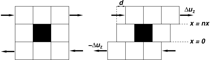
Figure 1: Our lattice-Boltzmann code LB3D implements shearing by use of Lees-Edwards boundary conditions: particles crossing the $\bf x=0=nx$ boundary have their $z$-velocities altered by $\pm\Delta u_{Z}$ and are displaced in the $\pm z$ direction by $d=t\Delta u_{Z}$ ($t$ = simulation time). The corresponding shear rate is $s=\Delta u_{Z}/nx$; oscillatory shear is achieved by setting $\Delta u_{Z}^{\prime}=\cos(\omega t)\Delta u_{Z}$.

We are applying our model to study spinodal decomposition under shear, also referred to as Couette flow. The phase separation of binary immiscible fluids without shear has been studied in detail by different authors and LB3D has been shown to model the underlying physics successfully [González-Segredo et al., 2003]. It has been shown in the non-sheared studies of spinodal decomposition that lattice sizes need to be large in order to overcome finite size effects, i.e. 128³ has been found the minimum acceptable number of lattice sites [González-Segredo et al., 2003]. For high shear rates, systems also have to be very long because, if the system is too small, the domains interconnect across the $\bf z=0$ and $\bf z=nz$ boundary and form interconnected lamellae in the direction of shear. Such artefacts need to be eliminated from our simulations.

Computational steering is a very useful tool for checking on finite size effects in an ongoing sheared fluid simulation. While being able to constantly monitor volume-rendered colour fields or fluid densities, the human eye turned out to be very reliable in spotting the moment when these simulations become unphysical. In this way, we were able to keep the computational resources required at a minimum.

From our studies we found that to avoid finite size effects 64x64x512 systems are sufficient for low shear rates and short simulation times, but 128x128x1024 lattices are needed for higher shear rates and/or very long simulations.

The results presented in this section were all obtained for a 64x64x512 system with all relaxation times and masses set to unity, i.e. $\tau^{\sigma}$=1.0, $m^{\sigma}$=1.0. The initial oil and water fluid densities $f_{r}$ and $f_{b}$ were given by a random distribution between 0.0 and 0.7 (in lattice units). All simulations were performed on 64 CPUs of a SGI Origin 3800 at CSAR in Manchester, UK. Shear rates $s$ were set to $0$, $7.8\times 10^{-4}$, $1.6\times 10^{-3}$, $3.1\times 10^{-3}$ and $4.7\times 10^{-3}$ (in lattice units) in order to study the influence of shear on the domain growth. In order to compare between different simulations, we define the time dependent lateral domain size $L(t)$ along direction $i=x,y,z$ as

$$L_{i}(t)\equiv\frac{2\pi}{\sqrt{\left<k^{2}_{i}(t)\right>}},$$ (11)

where

$$\left<k^{2}_{i}(t)\right>\equiv\frac{\sum_{\mathbf{k}}k_{i}^{2}S(\mathbf{k},t)}{\sum_{\mathbf{k}}S(\mathbf{k},t)}$$ (12)

is the second order moment of the three-dimensional structure function

$$S(\mathbf{k},t)\equiv\frac{1}{V}\left|\phi^{\prime}_{\mathbf{k}}(t)\right|^{2}$$ (13)

with respect to the cartesian component $i$. $\left<\right>$ denotes the average in Fourier space, weighted by $S(\mathbf{k})$ and $V$ is the number of nodes of the lattice, $\phi^{\prime}_{\mathbf{k}}(t)$ the Fourier transform of the fluctuations of the order parameter $\phi^{\prime}\equiv\phi-\left<\phi\right>$, and $k_{i}$ is the $i$th component of the wave vector.

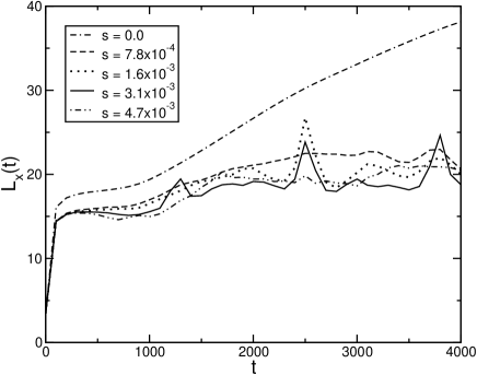
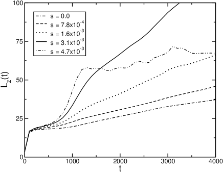
Figure 2: The time-dependent lateral domain size $L$ in $x$ (left) and $z$ directions (right) for different shear rates. Initial fluid densities are randomly distributed between 0 and 0.7, the system size is 64x64x512, and $\tau^{\sigma}=m^{\sigma}=1$ (all quantities are reported in lattice units).

Figure 2 shows the time dependent lateral domain size in $x$ and $z$ directions for the abovementioned parameters and up to 4000 timesteps. At the beginning of simulations, there is a steep increase of $L$ due to rapid diffusion of mass to nearest neighbours before the domain growth starts. As expected, the behaviour of $L(t)$ is identical in $x$ and $z$ directions for $s=0.0$, but is very different for $s>0.0$. The average slope of $L_{x}(t)$ decreases for increasing $s$ until phase separation almost arrests and multiple peaks occur for $s=1.6\times 10^{-3}$ and $s=3.1\times 10^{-3}$ (in lattice units). These peaks arise very regularly at approximately every 700 timesteps in the former case and every 1500 timesteps in the latter case. For $s=4.7\times 10^{-3}$ these peaks cannot be observed. They can be explained as follows: if a domain reaches a substantial size, the probability of it coalescing with a similarly sized one becomes high, but the resulting very large domain will be unable to withstand the strain caused by the shear and will break up a few timesteps later. For higher shear rates, domain growth in the $x$ direction is slower than for lower shear rates and the peaks occur with a smaller frequency. If $s$ becomes too high (as in the $s=4.7\times 10^{-3}$ case), the imposed strain prevents domains substantially larger than the average domain size from forming.

In the $z$ direction, shear causes elongated domains resulting in increasing values of $L(t)$ for increasing shear rates. For $s=4.7\times 10^{-3}$, $L_{z}(t)$ grows rapidly until it saturates at $t=1100$. A critical domain size is reached after which domains still grow, but are very elongated and tilted by an angle. Due to this tilting, $L_{z}$ saturates since it only measures the size of the domains in $z$ direction.

This effect is illustrated in figure 3 which shows volume-rendered snapshots of the order parameter $\phi$ for shear rates $s=0.0$, $1.6\times 10^{-3}$, and $4.7\times 10^{-3}$, all at timestep 3000. Areas of high density of ‘blue’ fluid are coloured blue and the interface between both fluids is coloured red. The figure shows how the domains develop evenly in $x$ and $z$ direction for $s=0.0$, but become tilted and elongated under shear. This effect increases with increasing shear rate, resulting in very long and slim lamellae in the $s=4.7\cdot 10^{-3}$ case.

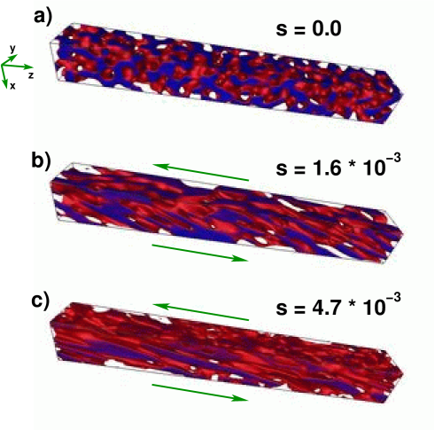
Figure 3: Volume rendered order parameter $\phi$ for increasing shear rates all shown at timestep 3000. The system size is 64x64x512. Blue areas denote high density of ‘blue’ fluid and red denotes the interface between fluids. With increasing shear rate, domains become more elongated and tilted.

The results presented in this section are preliminary. We hope to be able to report on more detailed studies of essentially finite-size-free simulations of complex fluid mixtures under shear in the near future. We are planning to utilize our code to quantify domain growth and compare our results to previous theoretical work and experimental results [Cates et al., 1999, Wagner and Yeomans, 1999, Corberi et al., 2002]. Applying oscillatory instead of constant shear is a natural extension of this work and simulations are already ongoing [Xu et al., 2003]. We are also studying the properties of amphiphilic fluid mixtures under shear including the effect shear has on previously formed cubic mesophases such as the ’P’-phase [Nekovee and Coveney, 2001] and the gyroid cubic mesophase [González-Segredo and Coveney, 2003]. Such complex fluids are expected to exhibit non-Newtonian properties.

6 Multiphase flow in porous media

The study of transport phenomena in porous media is of great interest in fields ranging from oil recovery and water purification to industrial processes like catalysis. In particular, the oilfield industry uses complex, non-Newtonian, multicomponent fluids (containing polymers, surfactants and/or colloids, brine, oil and/or gas), for processes like fracturing, well stimulation and enhanced oil recovery. The rheology and flow behaviour of these complex fluids in a rock is different from their bulk properties. It is therefore of considerable interest to be able to characterise and predict the flow of these fluids in porous media.

The flow of a single phase non-Newtonian fluid through two-dimensional porous media has been addresses with lattice-Boltzmann methods [Aharonov and Rothman, 1993, Chin et al., 2002], using a ‘top-down’ approach, in which the effective dynamic viscosity of the fluid, and hence the relaxation parameter in the BGK equation 5, explicitly depends on the strain rate tensor through a power law.

However, from the point of view of a modelling approach, the treatment of complex fluids in three-dimensional complex geometries is an ambitious goal. In this paper we shall only consider binary (oil/water) mixtures of Newtonian fluids, since this is a first and necessary step in the understanding of multiphase fluid flow in porous media.

The advantage of using lattice-Boltzmann (or lattice-gas) techniques in studying flow in porous media is that complex geometries can be easily implemented and the flow problem solved therein, since the evolution of the particle distribution functions can be described in terms of local collisions with the obstacle sites using simple bounce-back boundary conditions. Synchrotron based X-ray microtomography (XMT) imaging techniques provide high resolution, three-dimensional digitised images of rock samples. By using the lattice-Boltzmann approach in combination with these high resolution images of rocks, not only it is possible to compute macroscopic transport coefficients, such as the permeability of the medium, but information on local fields, such as velocity or fluid densities, can also be obtained at the pore scale thus providing a detailed insight into local flow characterisation and supporting the interpretation of experimental measurements [Auzerais et al., 1996].

The XMT technique measures the linear attenuation coefficient from which the mineral concentration and composition of the rock can be computed. From the tomographic image of the rock volume the topology of the void space can be derived, such as pore size distribution and tortuosity, and the permeability and conductivity of the rock can be computed [Spanne et al., 1994]. The tomographic data are represented by a reflectivity greyscale value and are arranged in voxels in a three dimensional coordinate system. The linear size of each voxel is defined by the imaging resolution, which is usually on the order of microns. By introducing a threshold to discriminate between pore sites and rock sites, these greyscale images can be reduced to a binary (0’s and 1’s) representation of the rock geometry. Using the lattice-Boltzmann method, single phase or multiphase flow can then be described in these real porous media.

Lattice Boltzmann and lattice gas techniques have already been applied to study single and multiphase flow through three-dimensional microtomographic reconstruction of porous media. For example, Martys and Chen [Martys and Chen, 1996] and Ferréol and Rothman [Ferréol and Rothman, 1995] studied relative permeabilities of binary mixtures in Fontainebleau sandstone. These studies validated the model and the simulation techniques, but were limited to small lattice sizes, of the order of $64^{3}$.

The possibility of describing fluid flow in real rock samples gives the advantage of being able to make comparisons with experimental results obtained on the same, or similar, pieces of rock. Of course, to achieve a reasonable comparison, the size of the rock used in lattice-Boltzmann simulations should be of the same order of magnitude as the system used in the experiments, or at least large enough to capture the rock’s topological features. The more inhomogeneous the rock, the larger the sample size needs to be in order to describe the correct pore distribution and connectivity. Another reason for needing to use large lattice sizes is the influence of boundary conditions and lattice resolution on the accuracy of the lattice-Boltzmann method. It has been shown (see for example [He et al., 1997], [Chen and Doolen, 1998] and references therein) that if the Bhatnagar-Gross-Krook (BGK) [Bhatnagar et al., 1954] approximation of the lattice-Boltzmann equation is used, the so-called bounce-back boundary condition at the wall sites actually mimics boundaries which move with a speed that depends on the relaxation parameter $\tau$ of the collision operator in the BGK equation (5). The relaxation parameter determines the kinematic viscosity of the simulated fluid. This implies that the computed permeability is a function of the viscosity.

The accuracy of lattice-Boltzmann simulations also depends on the Knudsen number which represents the ratio of the mean free path of the fluid particles and the characteristic length scale of the system (such as the pore diameter). To accurately describe hydrodynamic behaviour this ratio has to be small. If the pores are resolved with an insufficient number of lattice points finite size effects arise, leading to an inaccurate description of the flow field.

The error in solving the flow field increases with increasing viscosity (relaxation time), but this viscosity dependence becomes weak with increasing lattice resolution. Hence it is desirable to use a high resolution within the pore space in order to decrease the error induced by the use of bounce-back boundary conditions. However, increasing the resolution means increasing the lattice size, hence the computational cost of the simulation.

Boundary conditions other than bounce-back have been proposed and shown to give correct velocities at the boundaries. However these methods are either suitable only for flat interfaces [Inamuro et al., 1995] or they are cumbersome to implement [Verberg and Ladd, 2001], reducing the efficiency of the lattice-Boltzmann method.

Large lattices require a highly scalable code, access to high performance computing, terascale storage facilities and high performance visualisation. LB3D provides the first of these, while the others are now offered by the UK High Performance Computing services, and are also accessible via the UK e-Science Grid using RealityGrid capabilities.

Using LB3D and capability computing services provided by Manchester CSAR SGI Origin 3800, we were able to simulate drainage and imbibition processes in a $512^{3}$ subsample of Bentheimer sandstone X-ray tomographic data. The whole set of XMT data represented the image of a Bentheimer sandstone of cylindrical shape with diameter 4mm and length 3mm. The XMT data were obtained at the European Synchrotron Research Facility (Grenoble) at a resolution of $4.9\mu{\rm m}$, resulting in a data set of approximately 816x816x612 voxels. Figure 4 shows a snapshot of the $512^{3}$ subsystem.

The aim of this study is to compare velocity distributions with the ones measured by magnetic resonance imaging (MRI) of oil and brine infiltration into saturated Bentheimer rock core [Sheppard et al., 2003]. The rock sample used in these MRI experiments had a diameter of 38 mm and was 70 mm long; three-dimensional images of the rock were acquired at a resolution of 280 microns. The system size we used in lattice-Boltzmann simulations was smaller than the sample used in MRI experiments, but still of a similar order of magnitude and large enough to represent the rock geometry. On the other hand, the higher space resolution provided by the lattice-Boltzmann method permits a detailed characterisation of the flow field in the pore space, hence providing a useful tool to interpret the MRI experiments, for example in identifying regions of stagnant fluid. Detailed results of these lattice-Boltzmann simulations will be presented in a future paper.

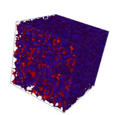
Figure 4: Rendering of an X-ray microtomographic image of a $512^{3}$ sample of Bentheimer sandstone. The data have a resolution of $4.9\mu m$. The pore space is shown in red, while the rock is represented in blue.

6.1 Binary flow in a digitised Bentheimer rock sample.

Darcy’s law [Darcy, 1856] for binary immiscible (oil/water) fluid mixtures was investigated and the dependence of the relative permeability coefficients on water saturation was derived and compared with lattice-gas studies. The extended Darcy’s law for binary flow takes the form

$${\bf J}_{i}=\sum_{j=1}^{2}k_{ij}(S)\frac{k}{\mu_{i}}{\bf X}_{j},\hskip 22.76228pt(i=1,2)$$ (14)

where ${\bf J}_{i}$ is the flux of the $i$th component and ${\bf X}_{j}$ is the force acting on the $j$th component. $k_{ij}(S)$ is the relative permeability coefficient depending on the saturation $S$, $k$ is the permeability of the medium and $\mu_{i}$ the viscosity of component $i$.

Using the lattice-Boltzmann method it is easy to selectively force only one component in a binary mixture, leaving the other one unforced. In this way the diagonal terms of the relative permeability matrix ($k_{ii}$) can be computed by analysing the flux of one component when it is forced, while the cross terms ($k_{ij}$) can be computed from the flux of one component when the other one is forced.

Since we want to study the flow behaviour for different forcing levels and for forcing applied in turn to both fluids, a large number of simulations is required. Hence we limited the size of our system to a subsample of 64x64x32 voxels, mirrored in the $z$-direction (flow direction) to give a final size of $64^{3}$ lattice sites (see figure 5). Periodic boundary conditions were applied in all directions.

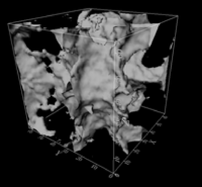
Figure 5: A $64^{3}$ sample of Bentheimer sandstone at a lattice resolution of $4.9\mu m$. The figure shows the isosurface delimiting the pore volume. The pore space is in the inner region of the isosurface.

Immiscible, binary mixtures of oil and water were flowed in this sample, at different forcing levels and by forcing in turn either the water or the oil component. In each of these numerical experiments, the system was initialised with a 50:50 mixture of oil and water, both given the same viscosity and the same initial density distributions. The rock walls were made fully water wettable, to reproduce experimental conditions and to discriminate between the two fluids which would otherwise be equivalent. The rock wettability is implemented by assigning each rock site a density distribution equal to the initial density of water. These density distributions do not flow, but exert a (repulsive) force on the oil component, pushing it away from the rock walls.

As the two components flow, they initially phase separate and, after some time, a steady state is reached. Here we are only interested in the velocity field at the steady state. If the total time allocated for the simulation is longer than the time needed to reach the steady state, we would waste CPU time performing calculations which are useless. If we run a simulation for less time than needed to reach the steady state, using the checkpoint-restart facility within LB3D we can resume the simulation and continue the run until the steady state is reached. In both cases, steering improves the efficiency of the runs. By steering we can dump velocity and density fields at variable frequency, check whether the fields at two different times differ or not, and in case their difference is less than a given threshold, decide that the steady state is reached and stop the simulation. In the simulations presented here an average of 15000 time steps is needed to reach the steady state. At this time the total flux (normalised by the pore volume) can be computed.

Figure 6 shows the force/flux dependence for the forced fluids. The linearity of force/flux holds for all the forcing levels considered. At any given forcing level, the wetting fluid flows less than the non-wetting one. This is due to the fact that the wetting fluid interacts with the rock walls, and adheres to them, hence exerting more resistance to flow, while the non-wetting fluid is lubricated by the wetting fluid. Similar results have been achieved in three-dimensional lattice-gas studies of binary flow in Fontainebleau sandstone [Love et al., 2001, Olson and Rothman, 1997]. A difference between our results and the lattice-gas ones is that in the latter the authors observed the presence of a capillary threshold, a minimum forcing level required to make the non-wetting fluid flow, while here we observe flow even at small forcing levels. The presence of this threshold is due to geometric constraints imposed by the distribution and size of rock pores and throats, which can trap bubbles of the non wetting fluid. In the rock sample we used for this study there are no such narrow throats, hence we would not expect to observe any capillary threshold.

In figure 6 the force/flux relation is plotted for the non-forced fluids. In this case at any applied forcing the non wetting fluid flows more than the wetting one. For the non wetting fluid we observe viscous coupling, i.e. the fluid flows even if it is not directly forced, and Darcy’s linearity is found for all forcing levels. On the other hand, the wetting fluid does not flow until a sufficiently high force is applied. This is due to the capillary forces. Hence Darcy’s law is observed to hold only for sufficiently high forcing.

From the linear regime regions in both graphs we computed the relative permeability coefficients: $k_{\rm ww}=1.6$, $k_{\rm oo}=3.3$, $k_{\rm ow}=0.77$, $k_{\rm wo}=0.57$, where the subscripts indicate water (w) and oil (o). The diagonal terms are one order of magnitude larger than the cross terms, which can be expected because the cross terms represent the response of one fluid when the other one is forced. This is also in agreement with the results from lattice-gas studies [Love et al., 2001].

A previous much debated issue is whether the off-diagonal terms in the relative permeability matrix should satisfy a reciprocity relationship. The reciprocity of the coefficients in macroscopic linear transport laws of the form

$$J_{i}=\sum_{j}L_{ij}X_{j},$$ (15)

where $J_{i}$ is a current and $X_{j}$ is a force conjugate to the current, is a consequence of Onsager’s regression hypothesis and it holds for systems which are linearly perturbed from equilibrium [de Groot and Mazur, 1985].

Our results show a linear dependence between force and flow, but the off-diagonal coefficients we obtained from the linear regime region have slightly different values for the wetting and non-wetting fluids. For binary immiscible fluid flow in porous media, where complex interfacial dynamics plays a major role, it is not clear if Onsager’s theory can be applied. In the aforementioned lattice-gas studies, Onsager’s reciprocity was found, but no clear theoretical justification has been given for the reason that this should hold under the general nonlinear conditions pertaining [Flekkøy and Pride, 1999].

It can also be observed that there are no error bars provided with our results. This is due to the fact that in lattice-Boltzmann, as opposite to lattice-gas simulations, there is no noise, and indeed this is one of the major computational advantages of the method. Nevertheless, we plan to perform the same set of simulations starting from different initial conditions, which may lead to different fluid/fluid interfacial structures and fluid transport coefficients, and then derive error bars from the flow computed in each of these simulations. More studies on different pore space geometries and larger systems need to be done to address the general validity of Darcy’s law for binary mixtures and Onsager’s reciprocity hypothesis.

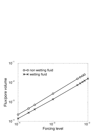
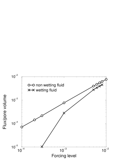
Figure 6: Flux of binary fluid when forced (a) and when unforced (b). All quantities are given in lattice units and the flux is normalised by the pore volume.

7 Conclusions

This paper describes optimal implementation of large scale lattice-Boltzmann simulations of two-phase fluid dynamics through exploitation of capability computing and computational steering. Capability computing promotes the execution of scalable codes that utilise a large fraction and sometime the entire allocation of processors on a big supercomputer. Computational steering then ensures that this massive set of resources is used optimally to generate meaningful scientific data. We illustrated the use of these approaches by reporting preliminary results from two applications which benefit substantially from large scale simulation. The first of these was concerned with Couette (shear) flow, where simulation cells of high aspect ratio are needed to eliminate finite size effects; the second described two-phase flow in large portions of digitised data obtained from X-ray microtomographic studies of Bentheimer sandstone. The most efficient utilisation of computational steering of such large scale simulations utilises a computational grid. These grids are in their infancy today and much more work needs to be done to render them transparent to users. Nevertheless, important advances have already been made, and here we described the grid-enablement of our lattice-Boltzmann codes. Our experience with grids to date leads us to conclude that much lighter middleware solutions will be required to foster their widespread use.

References

- Aharonov and Rothman, 1993 Aharonov, E. and Rothman, D. H.: 1993, Geophys. Research Lett. 20, 679
- Auzerais et al., 1996 Auzerais, F. M., Dunsmuir, J., Ferreol, B. B., Martys, N., Olson, J., Ramakrishnan, T., Rothman, D., and Schwartz, L.: 1996, Geophys. Research Lett. 23(7), 705
- Berman et al., 2003 Berman, F., Fox, G., and Hey, T.: 2003, Grid Computing: Making The Global Infrastructure a Reality, John Wiley and Sons
- Bhatnagar et al., 1954 Bhatnagar, P. L., Gross, E. P., and Krook, M.: 1954, Phys. Rev. 94(3), 511
- Brooke et al., 2003 Brooke, J. M., Coveney, P. V., Harting, J., Jha, S., Pickles, S. M., Pinning, R. L., and Porter, A. R.: 2003, in Proceedings of the UK e-Science All Hands Meeting, September 2-4, pp 885–889, (http://www.nesc.ac.uk/events/ahm2003/AHMCD/pdf/179.pdf)
- Cates et al., 1999 Cates, M. E., Kendon, V. M., Bladon, P., and Desplat, J. C.: 1999, Faraday Disc. 112, 1
- Chapman and Cowling, 1952 Chapman, S. and Cowling, T. G.: 1952, The Mathematical Theory of Non-Uniform Gases, Cambridge University Press, second edition
- Chen et al., 2000 Chen, H., Boghosian, B. M., Coveney, P. V., and Nekovee, M.: 2000, Proc. R. Soc. Lond. A 456, 2043
- Chen and Doolen, 1998 Chen, S. and Doolen, G. D.: 1998, Annu. Rev. Fluid Mech. 30, 329
- Chin et al., 2002 Chin, J., Boek, E. S., and Coveney, P. V.: 2002, Proc. R. Soc. Lond. A 360, 547
- Chin et al., 2003 Chin, J., Harting, J., Jha, S., Coveney, P. V., Porter, A. R., and Pickles, S. M.: 2003, Contemporary Physics 44(5), 417
- Corberi et al., 2002 Corberi, F., Gonnella, G., and Lamura, A.: 2002, Phys. Rev. E 66(016114)
- Coveney, 2003 Coveney, P. V.: 2003, Phil. Trans. R. Soc. Lond. A 361(1807), 1057
- Darcy, 1856 Darcy, H.: 1856, Les Fontaines Publiques de la Ville de Dijon, Dalmont, Paris
- de Groot and Mazur, 1985 de Groot, S. R. and Mazur, P.: 1985, Nonequilibrium thermodynamics, Dover Publications Inc., New York
- Ferréol and Rothman, 1995 Ferréol, B. and Rothman, D. H.: 1995, Transport in porous media 20, 3
- Flekkøy and Pride, 1999 Flekkøy, E. G. and Pride, S. E.: 1999, Phys. Rev. E 60(4), 4130
- Foster and Kesselman, 1999a Foster, I. and Kesselman, C.: 1999a, in I. Foster and C. Kesselman (eds.), The Grid: Blueprint for a New Computing Infrastructure, pp 15–25, Morgan Kaufmann
- Foster and Kesselman, 1999b Foster, I. and Kesselman, C.: 1999b, in I. Foster and C. Kesselman (eds.), The Grid: Blueprint for a New Computing Infrastructure, p. 259, Morgan Kaufmann
- González-Segredo and Coveney, 2003 González-Segredo, N. and Coveney, P. V.: 2003, e-print: www.arXiv.org/cond-mat/0310390
- González-Segredo et al., 2003 González-Segredo, N., Nekovee, M., and Coveney, P. V.: 2003, Phys. Rev. E 67(046304)
- Harting et al., 2003 Harting, J., Wan, S., and Coveney, P. V.: 2003, Capability Computing: The newsletter of the HPCx community 2
- He et al., 1997 He, X., Q. Zou, L. L., and Dembo, M.: 1997, J. Stat. Phys. 87(115),
- Inamuro et al., 1995 Inamuro, T., Yoshino, M., and Ogino, F.: 1995, Phys. Fluids 7(12), 2928
- Kendon et al., 2001 Kendon, V. M., Cates, M. E., Pagonabarraga, I., Desplat, J. C., and Bladon, P.: 2001, J. Fluid Mech. 440, 147
- Lees and Edwards, 1972 Lees, A. W. and Edwards, S. F.: 1972, J. Phys. C. 5(15), 1921
- Liboff, 1990 Liboff, R. L.: 1990, Kinetic Theory: Classical, Quantum, and Relativistic Descriptions, Prentice-Hall
- Love et al., 2001 Love, P. J., Maillet, J., and Coveney, P. V.: 2001, Phys. Rev. E 64(061302)
- Love et al., 2003 Love, P. J., Nekovee, M., Coveney, P. V., Chin, J., González-Segredo, N., and Martin, J. M. R.: 2003, Comp. Phys. Comm. 153(3), 340
- Martys and Chen, 1996 Martys, N. S. and Chen, H.: 1996, Phys. Rev. E 53(1), 743
- Nekovee et al., 2001 Nekovee, M., Chin, J., González-Segredo, N., and Coveney, P. V.: 2001, in E. Ramos et al (ed.), Computational Fluid Dynamics, Proceedings of the Fourth UNAM Supercomputing Conference, Singapore, pp 204–212, World Scientific
- Nekovee and Coveney, 2001 Nekovee, M. and Coveney, P. V.: 2001, J. Am. Chem. Soc. 123(49), 12380
- Olson and Rothman, 1997 Olson, J. F. and Rothman, D. H.: 1997, J. Fluid Mech. 341, 343
- Shan and Chen, 1993 Shan, X. and Chen, H.: 1993, Phys. Rev. E 47(3), 1815
- Sheppard et al., 2003 Sheppard, S., Mantle, M., Sederman, A., Johns, M., and Gladden, L. F.: 2003, Magnetic Resonance Imaging 21, 365
- Spanne et al., 1994 Spanne, P., Thovert, J. F., Jacquin, C. J., Lindquist, W. B., Jones, K. W., and Adler, P. M.: 1994, Phys. Rev. Lett. 73(14), 2001
- Succi, 2001 Succi, S.: 2001, The Lattice Boltzmann Equation for Fluid Dynamics and Beyond, Oxford University Press
- Verberg and Ladd, 2001 Verberg, R. and Ladd, A. J. C.: 2001, Phys. Rev. E 65,
- Wagner and Pagonabarraga, 2002 Wagner, A. J. and Pagonabarraga, I.: 2002, J. Stat. Phys. 107, 521
- Wagner and Yeomans, 1999 Wagner, A. J. and Yeomans, J. M.: 1999, Phys. Rev. E 59(4), 4366
- Xu et al., 2003 Xu, A., Gonnella, G., and Lamura, A.: 2003, Phys. Rev. E 67(056105)