A Matrix Kato-Bloch Perturbation Method for Hamiltonian Systems

Abstract

A generalized version of the Kato-Bloch perturbation expansion is presented. It consists of replacing simple numbers appearing in the perturbative series by matrices. This leads to the fact that the dependence of the eigenvalues of the perturbed system on the strength of the perturbation is not necessarily polynomial. The efficiency of the matrix expansion is illustrated in three cases: the Mathieu equation, the anharmonic oscillator and weakly coupled Heisenberg chains. It is shown that the matrix expansion converges for a suitably chosen subspace and, for weakly coupled Heisenberg chains, it can lead to an ordered state starting from a disordered single chain. This test is usually failed by conventional perturbative approaches.

Since its introduction long ago by Rayleigh and Schrödinger, the perturbation method has become an essential tool for the analysis of Hamiltonians. The perturbative method consists in searching for an approximate solution of the eigenvalue equation of a linear operator slightly different from an unperturbed operator whose spectrum is known. In the perturbation expansion it is assumed that, if the system Hamiltonian is written as the sum of two parts $H=H_{0}+gV$, where $H_{0}$ is the unperturbed Hamiltonian and $gV$ the perturbation, the perturbed energies and eigenfunctions are power series of $g$. The convergence of these series was studied by mathematicians kato_BOOK , whose work may be summarized by two important results.

Let $A$ be a unitary space (i.e., a Hilbert space or more generally a Banach space). The eigenvalues of $H$ satisfy the characteristic equation $det(H-\lambda)=0$. This is an algebraic equation of degree $N$ equal to the dimension of $A$, $N=dimA$. Its coefficients are holomorphic functions of $g$. The first result is given by the following theorem: the roots $\lambda$ of $det(H-\lambda)=0$ constitute one or several branches of analytic functions of $g$ with only algebraic singularities. The second result is a theorem due to Rellich kato_BOOK , and may be stated as follows: the power series for an eigenstate or an eigenvalue of $H$ are convergent if the magnitude of the perturbation $|gV|$ is smaller than half of the isolation distance of the corresponding unperturbed eigenvalue. In other terms, if an eigenvalue of $H_{0}$ is isolated from the rest of the spectrum then, for a sufficiently small $g$, the expansion will converge.

These results have been known for a long period of time. But they are barely mentioned in numerous works in condensed matter theory or in high energy theory in which perturbation expansions are used. This is because, in most problems, one is mainly interested in one or two-particle properties. Hence, perturbation expansions were formulated in terms of single or two-particle Green’s functions of the unperturbed Hamiltonian nozieres . The convergence properties of Green’s function is very tedious to analyze. One has to sum up complicated classes of infinite series of Feyman diagrams, in the so-called parquet summation, without a clear selection criterion. This type of expansion generally leads to the divergence of the dominant quantum fluctuations at low temperatures. This indicates the onset of long-range order, but, the ordered state cannot be reached. Reaching the ordered state may necessitate going across energy levels or a singularity. This is impossible with the conventional perturbation expansion which assumes the ground-state energy to be an analytic function of $g$. This has lead to the widespread belief that the spectrum of $H_{0}$ (which is supposed to describe a disordered phase) is not a good starting point if one wishes to reach the ordered phase. But a clear mathematical criterion on the convergence of the Green’s function series has never been provided. Hence, the Green’s function method simplifies the mathematics of the problem by reducing the many-body problem to a one- or two-body problem, but, it blurs the analysis of eventual convergence problems.

It could thus be better to analyze the perturbative expansions of Hamiltonians in the light of the above two theorems by using stationary perturbation instead of Green’s functions. However it is clear that if $H_{0}$ is the hopping Hamiltonian as used in Fermi systems, the Rellich theorem does not apply. This is because the spectrum is gapless and thus any perturbation, no matter how small, will not fullfil the convergence condition. That is why it is crucial to work in a finite volume. But, even in this case, most perturbation expansions do not converge if the system is large for reasonable values of $g$.

In this letter, a simple cure for the convergence problems of perturbative expansions defined in a finite volume is proposed. The starting point is the general perturbative expansion derived by Kato kato and Bloch bloch . The new method consists in replacing the original Kato-Block simple polynomial series by a matrix expansion. In the matrix expansion, the low lying excited states are used to shield the ground state from the rest of the spectrum so that the near degeneracy problems that usually plague conventional perturbation expansions are avoided. Arguments, but not a mathematical demonstration, of the convergence of the matrix expansion are given. The method is tested in some simple cases including the Mathieu equation and the anharmonic oscillator. Then, the new method is applied to weakly coupled antiferromagnetic (AFM) chains, a problem of high current interest in the physics of low-dimensional magnetic materials scalapino ; schulz . It is shown that, starting from a disordered ground state of a single chain, the new matrix perturbation is able to reach the ordered state when a small exchange interaction is turned on between the chains.

The Kato-Bloch expansion, for the correction ${\tilde{E}}_{0}$ to an eigenset ($E_{0}$, $|\phi_{0}\rangle$), which is supposed to be non-degenerate, is given by messiah :

$$P_{0}{\tilde{E}}_{0}P_{0}=P_{0}H_{0}P_{0}+gP_{0}VP_{0}+g^{2}P_{0}V{\tilde{Q}}_{0}VP_{0}+...$$ (1)

where $P_{0}=|\phi_{0}\rangle\langle\phi_{0}|$, and

$${\tilde{Q}}_{0}=\sum_{n>0}\frac{|\phi_{n}\rangle\langle\phi_{n}|}{E_{0}-E_{n}}.$$ (2)

When the problem is projected onto the subspace generated by the eigenstate $\phi_{0}$, one retrieves the perturbative series

$${\tilde{E}}_{0}=E_{0}+g\langle\phi_{0}|V|\phi_{0}\rangle+g^{2}\sum_{n>0}\frac{|\langle\phi_{0}|V|\phi_{n}\rangle|^{2}}{E_{0}-E_{n}}+...$$ (3)

Figure 1: Sketch of the separation of the spectrum in two regions.

In the expansion of ( 3), higher order correction terms to the ground state energy ${\tilde{E}}_{0}$ are governed by the ratio $g/(E_{1}-E_{0})$. Kato showed that if $g/(E_{1}-E_{0})<1/2$, then, the series converges. The problem that may lead to convergence failure of the perturbative series is easy to see in the Kato-Bloch formulation: the series diverges if $g/(E_{1}-E_{0})>1/2$. When this occurs, it is possible to eliminate the problem by formulating the expansion ( 1) in terms of matrices. This can lead to convergence for a suitable size of the matrices. The idea behind the matrix expansion is to shield $E_{0}$ from the rest of the spectrum in the expansion (Fig. 1). i.e., instead of restricting $P_{0}$ to the eigenvalue of interest $E_{0}$, one also includes a few excited states above $E_{0}$ up to the cut-off energy $E_{n_{c}}$. In the matrix method, $P_{0}$ is now given by

$$P_{0}=\sum_{n}^{n_{c}}|\phi_{n}\rangle\langle\phi_{n}|,$$ (4)

and the complement of the projector which enters into the perturbation expansion is

$${\tilde{Q}}_{0}=\sum_{n>n_{c}}\frac{|\phi_{n}\rangle\langle\phi_{n}|}{E_{0}-E_{n}}.$$ (5)

In this case, when the problem is projected onto the subspace generated by the $\phi_{n}$, $n=0,...,n_{c}$, each term in the expansion of the corrected energy of ( 3) is replaced by a matrix. Now, the largest term of order $k$ in the matrix expansion is $g^{k}/(E_{n_{c}+1}-E_{0})^{k-1}$ instead of $g^{k}/(E_{1}-E_{0})^{k-1}$ so that the condition $g/(E_{n_{c}+1}-E_{0})<1/2$ is fulfilled for a suitable chosen $n_{c}$.

If the matrix method is used with truncation to two states $E_{0}$ and $E_{1}$, the Kato-Block matrix expansion leads to the Hamiltonian ${\tilde{H}_{0}}$ given by

$${\tilde{H}}_{0}\approx\left(\begin{array}[]{cc}E_{0}&0\\ 0&E_{1}\end{array}\right)+g\left(\begin{array}[]{cc}V_{00}&V_{01}\\ V_{10}&V_{11}\end{array}\right)-$$ (10)

$$g^{2}\left(\begin{array}[]{cc}V_{00}^{(2)}&V_{01}^{(2)}\\ V_{10}^{(2)}&V_{11}^{(2)}\end{array}\right)+...,$$ (13)

where the second order matrix elements projected to the two states kept in the matrix expansion are respectively

$$V_{00}^{(2)}=\sum_{n>1}\frac{V_{0n}^{2}}{E_{n}-E_{0}},$$ (14)

$$V_{01}^{(2)}=\sum_{n>1}\frac{V_{0n}V_{1n}}{E_{n}-E_{0}},$$ (15)

$$V_{11}^{(2)}=\sum_{n>1}\frac{V_{1n}^{2}}{E_{n}-E_{0}}.$$ (16)

In the matrix expansion of ( 13), the eigenvalue of interest $E_{0}$ is now shielded from the rest of the spectrum by $E_{1}$. The solution of the eigenproblem for ${\tilde{H}}_{0}$ generally leads to a non-polynomial dependence of ${\tilde{E}}_{0}$ as a function of $g$. For instance, the first order corrected ground state energy for the matrix method is given by the expression

$${\tilde{E}}_{0}=\frac{1}{2}(E_{0}+gV_{00}+E_{1}+gV_{11})-$$

$$\frac{1}{2}\sqrt{E_{1}+gV_{11}-E_{0}-gV_{00}+4g^{2}V_{01}^{2}}.$$ (17)

It is clear that if $g/(E_{1}-E_{0})\gtrsim 1/2$, the expansion ( 3) will diverge while the expression of ${\tilde{E}}_{0}$ in ( 17) is well defined, i.e. non-trivial effects are already included into ${\tilde{E}}_{0}$ at the first order of the matrix expansion.

Let us now study a few models in order to illustrate the difference between the matrix method and the simple polynomial expansion. It is interesting to first study the Mathieu equation which arises, for instance, after separation of variables of Laplace’s equation in elliptic cylindrical coordinates. This is because this equation was actually used by Bloch bloch as a test for the polynomial expansion. The Mathieu equation is

$$(-\frac{d^{2}}{d\theta^{2}}+g\cos^{2}\theta)\phi(\theta)=E\phi(\theta).$$ (18)

This equation may be studied by perturbation theory with $d^{2}/d\theta^{2}$ as the $H_{0}$ and $g\cos^{2}\theta$ as the perturbation. The eigenvalues $E_{n}$ and eigenfunctions $\phi_{n}$ of the free part which are even functions with period $\pi$ are $E_{n}=n^{2}$ and $\phi_{n}=1/\sqrt{\pi}\cos n\theta$ where $n=0,2,4...$. The correction to the groundstate energy obtained from the original Bloch method up to the fourth order is

$${\tilde{E}}_{0}^{(4)}=\frac{g}{2}-\frac{1}{2}(\frac{g}{4})^{2}+\frac{7}{128}(\frac{g}{4})^{4}+O(g^{5}).$$ (19)

$g$	Bloch	$m=2$	$m=4$	$m=8$	exact
0.5	0.242201	0.242203	0.242201	0.242201	0.242201
1	0.468964	0.468910	0.468961	0.468961	0.468961
2	0.878418	0.878680	0.878234	0.878234	0.878234
4	1.554688	1.550510	1.544861	1.544861	1.544861
8	2.875000	2.535818	2.486044	2.486044	2.486044
16	14.000000	4.000000	3.719515	3.719481	3.719481

Table 1: Fourth order simple expansion from ( 19) (Bloch) versus first order matrix expansion for $m=2,4,8$ states kept in for the lowest state of the Mathieu equation.

Table 1 compares the correction obtained from ( 19) with the matrix perturbation theory and the exact result. When $g\lesssim 2$, the condition $g/(E_{1}-E_{0})<1/2$ is fulfilled, both the first order matrix perturbation result even for a small number of states $m$, and the fourth order perturbation estimate of ( 19), shown in Table 1, agree quite well with the exact solution. One may note that the first order simple perturbation estimate is $0.250000$. At this level, the first order simple perturbation and first order matrix perturbation are already different as explained above. When $g\gtrsim 4$, $g/(E_{1}-E_{0})\gtrsim 1$ the simple perturbation series diverges and ( 19) cannot be used to compute the correction to the ground state energy. The difference between the simple perturbation and the exact result increases with increasing $g$. In contrast, the matrix perturbation method leads to good results up to $g=16$ even if a small number of states is kept in the construction of $P_{0}$. The agreement with the exact result extends to more than the sixth digit when eight or more states are kept. The matrix perturbation estimate can be improved for a fixed number of states by increasing the order of the matrix series. For instance in Table 2, when a second order term is included for $m=2$, the agreement with the exact result is better. In the Mathieu equation, the rapid convergence of the matrix method is due to the fact that the energy separation between consecutive eigenvalues is roughly $(n+2)^{2}-n^{2}$. Thus, the condition $g/(E_{n_{c}+1}-E_{0})<1/2$ can easily be satisfied.

$g$	$m=2$(1)	$m=2$(2)	exact
0.5	0.242203	0.242201	0.242201
1	0.468910	0.468961	0.468961
2	0.878680	0.878231	0.878234
4	1.550510	1.544708	1.544861
8	2.535818	2.481531	2.486044
16	4.000000	3.647650	3.719481

Table 2: First order(1) versus second order (2) 2-state matrix expansion for the lowest state of the Mathieu equation.

Let us now consider the case of an harmonic oscillator with a quartic perturbation which does not present this advantage. The Hamiltonian is

$$H_{osc}=\frac{1}{2}(p^{2}+q^{2})+gq^{4}.$$ (20)

In the Dirac notations, $H_{osc}$ becomes

$$H_{osc}=a^{\dagger}a+\frac{1}{2}+\frac{g}{4}(a^{4}+a^{\dagger 4}+4a^{\dagger 3}a+4a^{\dagger}a^{3}+$$

$$6a^{\dagger 2}a^{2}+6a^{2}+6a^{\dagger 2}+12a^{\dagger}a+3).$$ (21)

The unperturbed energies are now $E_{n}=0$, $1$, $2$,…This model has widely been used to test different perturbative approaches. It is now well established that the simple Brillouin-Wigner series is divergent for this model. One has to resort to special resummation procedures in order to obtain convergence. Table 3 shows that a simple first order matrix approach can accurately reproduce the exact result up to six digits for a modest number of states kept. But as expected, since the energy separation is $1$, a larger $m$ than in the Mathieu equation needs to be used in order to achieve the same accuracy.

$g$	$m=4$	$m=8$	$m=16$	$m=32$	exact
0.1	0.559564	0.559165	0.559146	0.559146	0.559146
0.3	0.640354	0.638539	0.637992	0.637992	0.639992
0.5	0.706301	0.697454	0.696178	0.696176	0.696176
1.0	0.855087	0.805870	0.803837	0.803771	0.803771
2.0	1.137219	0.956286	0.952468	0.951571	0.951568

Table 3: First order matrix expansion results for $m=4,8,16,32$ states kept compared to the exact result of reference janke for the lowest state of anharmonic oscillator.

Let us now consider a non-trivial model, antiferromagnetic (AF) Heisenberg chains weakly coupled by a ferromagnetic transverse exchange $J_{\perp}<0$. In this problem, $H_{0}=H_{\parallel}$ is an array of decoupled AF chains. When the conventional random phase approximation (RPA) is applied to this problem, one finds that the spin suceptibility diverges at low temperatures for any small $J_{\perp}$. This indicates that the ground state is ordered as soon as $J_{\perp}\neq 0$. But starting from the disordered chain, the ordered regime cannot be reached by RPA. It is necessary to turn to special procedures such as the chain-mean field approach scalapino ; schulz in which the existence of long-range order is assumed. It will now be shown below that the matrix Kato-Bloch method can reach the ordered regime without assuming long-range order a priori.

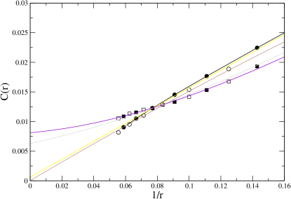
Figure 2: The ground state correlation function $C(r)={\bar{C}}_{\parallel}(25,25,r)$ for the $48\times 49$ lattice for $J_{\perp}=0$ (circles) and $J_{\perp}=-0.16$ (squares). The filled and open symbols correspond to odd and even distances respectively.

The exact spectrum of a single AF chain is known from the Bethe ansatz, but eigenfunctions are not easily accessible. Thus, the density-matrix renormalization group (DMRG) method white will be used to compute an approximate spectrum $\epsilon_{n},|\phi_{n}\rangle$ of a single chain. A preliminary account of the first order of this approach moukouri_TSDMRG as well as an extensive comparison with the Quantum Monte Carlo method was presented elsewhere moukouri_TSDMRG2 . By expressing the Hamiltonian on the basis generated by the tensor product of the states of different chains one obtains, up to the second order, the effective one-dimensional Hamiltonian,

$$\tilde{H}\approx\sum_{[n]}E_{\parallel[n]}|\Phi_{\parallel[n]}\rangle\langle\Phi_{\parallel[n]}|+J_{\perp}\sum_{l}{\bf\tilde{S}}_{l}{\bf\tilde{S}}_{l+1}-$$

$$\frac{J_{\perp}^{2}}{2}\sum_{l}{\bf S}_{l}^{(2)}{\bf S}_{l+1}^{(2)}+...$$ (22)

where the chain-spin operators on the chain $l$ are ${\bf\tilde{S}}_{l}=({\bf\tilde{S}}_{1l},{\bf\tilde{S}}_{2l},...{\bf\tilde{S}}_{Ll})$ and ${\bf S}_{il}^{(2)}=({\bf\tilde{S}}_{1l}^{(2)},{\bf\tilde{S}}_{2l}^{(2)},...{\bf\tilde{S}}_{Ll}^{(2)})$, $L$ is the chain length. The matrix elements of the first and second order local spin operators are respectively

$${\bf\tilde{S}}_{i,l}^{n_{l},m_{l}}=\langle\phi_{n_{l}}|{\bf S}_{i,l}|\phi_{m_{l}}\rangle,$$

$${\bf S}_{il}^{(2)n_{l}n^{\prime}_{l}}=\sum_{m_{l}}\frac{{\tilde{S}}_{il}^{n_{l}m_{l}}{\tilde{S}}_{il}^{m_{l}n^{\prime}_{l}}}{\sqrt{\epsilon_{m_{l}}-\epsilon_{0_{l}}}}.$$ (23)

The spectrum of the effective Hamiltonian ( 22) which is one-dimensional is also obtained by applying the DMRG. It is to be emphasized that the use of the DMRG here stems from the one-dimensionality of the effective problem. But in general, it is not necessary to apply this technique. $m=80$ states were kept which leads to $J_{\perp}/(E_{n_{c}+1}-E_{0})\approx 0.26$ for $J_{\perp}=-0.16$, which means the Rellich theorem is satisfied. Fig.( 2) shows the spin-spin correlation function parallel to the chains, ${\bar{C}}_{\parallel}(25,25,r)=\langle{\bf S(0)S(r)}\rangle/3$ for the middle chain $l=25$, the origin taken on site $i=25$ in the $48\times 49$ lattice, for the cases $J_{\perp}=0$ and $J_{\perp}=-0.16$. It is clearly seen that, as expected, the former extrapolate to zero. The same behavior is observed on $32\times 33$ and $64\times 65$ lattices. But when $J_{\perp}=-0.16$ the extrapolated value is finite. This indicates the presence of long-range order. The same behavior is observed on $32\times 33$ and $64\times 65$ lattices (not shown). The effect of the other chains is to create an effective magnetic field on the middle chain which leads to a finite order parameter. This result thus justifies the assumption behind chain mean-field theory approaches scalapino ; schulz .

In summary, using a somewhat loose interpretation of the Rellich theorem, a convergent matrix perturbation approach has been proposed. This new method, which treats both the ordered and disordered regimes in a controlled way, opens new possibilities in the study of phase transitions and strongly correlated electron in condensed-matter systems. The new method may also be useful in handling infrared divergences in light-front Hamiltonians in quantum chromodynamics wilson .

- (1) T. Kato, Perturbation Theory for Linear Operators, Classics in Mathematics, Springer (1980).
- (2) P. Nozières, Theory of Interacting Fermi Systems, Advanced Book Classics, Addison Wesley (1997).
- (3) T. Kato, Prog. Teor. Phys. 4, 514 (1949); 5, 95 (1950).
- (4) C. Bloch, Nucl. Phys. 6, 329 (1958).
- (5) D.J. Scalapino, Y. Imry, and P. Pincus, Phys. Rev. B 11, 2042 (1975).
- (6) H.J. Schulz, Phys. Rev. Lett. 77, 2790 (1996).
- (7) A. Messiah ’Quantum Mechanics’, Ed. Dover, p. 685-720 (1999).
- (8) W. Janke and H. Kleinert, Phys. Rev. Lett. 75, 2787 (1995).
- (9) S.R. White, Phys. Rev. Lett. 69, 2863 (1992). Phys. Rev. B 48, 10 345 (1993).
- (10) S. Moukouri and L.G. Caron, Phys. Rev. B 67, 092405 (2003).
- (11) S. Moukouri cond-mat/0305608 (unpublished).
- (12) S.D. Glazek and K.G. Wilson, Phys. Rev. D 49, 4214 (1994).