Hyperfine quenching of the metastable ${}^{3}\!P_{0,2}$ states in divalent atoms

Abstract

Hyperfine quenching rates of the lowest-energy metastable ${}^{3}\!P_{0}$ and ${}^{3}\!P_{2}$ states of Mg, Ca, Sr, and Yb atoms are computed. The calculations are carried out using ab initio relativistic many-body methods. The computed lifetimes may be useful for designing novel ultra-precise optical clocks and trapping experiments with the ${}^{3}\!P_{2}$ fermionic isotopes. The resulting natural widths of the ${}^{3}\!P_{0}-^{1}\!S_{0}$ clock transition are 0.44 mHz for ²⁵Mg, 2.2 mHz for ⁴³Ca, 7.6 mHz for ⁸⁷Sr, 43.5 mHz for ¹⁷¹Yb, and 38.5 mHz for ¹⁷³Yb. Compared to the bosonic isotopes, the lifetime of the ${}^{3}\!P_{2}$ states in fermionic isotopes is noticeably shortened by the hyperfine quenching but still remains long enough for trapping experiments.

I Introduction

This work is motivated by emerging experiments with cold divalent atoms Mg, Ca, Sr and Yb Cop . For example, the recently attained Bose-Einstein condensate of the ground-state Yb Takasu et al. (2003) may offer new insights into the physics of degenerate quantum gases due to a vast number of available isotopes and relative simplicity of molecular potentials. As to the ${}^{3}\!P_{2}$ metastable states (see Fig. 1), it was realized that the non-scalar nature of the ${}^{3}\!P_{2}$ states may be used to overcome the unfeasibility of magnetic trapping of the spherically-symmetric ${}^{1}\!S_{0}$ ground states Katori et al. (2001); Nagel et al. (2003); Xu et al. (2003); Grünert and Hemmerich (2002). Knowing radiative lifetimes of the other, ${}^{3}\!P_{0}$, metastable states is required in developing the next generation of ultraprecise optical atomic clocks Katori et al. (2003); Courtillot et al. (2003); Park and Yoon (2003); Porsev et al. (2003). Here the clockwork is based on cold atoms confined to sites of an engineered optical lattice. The lifetime determines the natural width of the clock transition between the ground and the ${}^{3}\!P_{0}$ state.

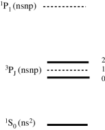
Figure 1: Lowest-lying energy levels of Mg ($n$=3), Ca ($n$=4), Sr ($n$=5), and Yb ($n$=6), relevant to the radiative decay of the $nsnp\,^{3}\!P_{0,2}$ states. The hyperfine quenching predominantly is caused by the admixture of the $nsnp\,^{3}\!P_{1}$ and $nsnp\,^{1}\!P_{1}$ states.

For all bosonic isotopes of Mg, Ca, Sr, and Yb, the nuclear spin $I$ vanishes and these isotopes lack hyperfine structure. For bosonic isotopes the ${}^{3}\!P_{0}$ state may decay only via very weak multi-photon (e.g., E1-M1) transitions. However, for fermionic isotopes (Table 1), $I\neq 0$, a new radiative decay channel becomes available due to the hyperfine interaction (HFI). The HFI, although small, admixes atomic levels of the total angular momentum $J=1$ thus opening an electric-dipole branch to the ground state. The resulting HFI-induced E1 decays do determine the lifetimes of the ${}^{3}\!P_{0}$ states. As to the ${}^{3}\!P_{2}$ states, here the single-photon decays are allowed, but being of non-E1 character, are very weak. The lifetimes are long and range from 15 seconds for Yb to 2 hours for Ca Porsev et al. (1999a); Derevianko (2001). As we demonstrate here, depending on an isotope, the hyperfine quenching of the ${}^{3}\!P_{2}$ states is either comparable to or is much faster than the small non-E1 rates.

Table 1: Nuclear parameters of the stable fermionic isotopes of Mg, Ca, Sr, and Yb. Here $I$ are the nuclear spins and $\mu/\mu_{N}$ are the nuclear magnetic moments expressed in units of the nuclear magneton $\mu_{N}$.

Isotope	$I$	$\mu/\mu_{N}$
25Mg	5/2	-0.85546
43Ca	7/2	-1.31727
87Sr	9/2	-1.09283
171Yb	1/2	0.4919
173Yb	5/2	-0.6776

A detailed theoretical analysis of the hyperfine quenching has been limited so far to astrophysically-important He, Be and Mg and their isoelectronic sequences Garstang (1962); Johnson et al. (1997); Brage et al. (1998, 2002). The hyperfine quenching of the ${}^{3}P_{0}$ states of Sr and Yb has been estimated in Refs. Katori et al. (2003); Porsev et al. (2003). Here we carry out ab initio relativistic many-body atomic structure calculations to extend and refine these previous studies. We find that the resulting natural widths of the ${}^{3}\!P_{0}-^{1}\!S_{0}$ clock transition are 0.44 mHz for ²⁵Mg, 2.2 mHz for ⁴³Ca, 7.6 mHz for ⁸⁷Sr, 43.5 mHz for ¹⁷¹Yb, and 38.5 mHz for ¹⁷³Yb. Compared to the bosonic isotopes, the lifetime of the ${}^{3}\!P_{2}$ states in fermionic isotopes is noticeably shortened by the hyperfine quenching but still remains long enough for trapping experiments.

The paper is organized as follows. First, in Section II we derive the hyperfine quenching rates using perturbation theory. The solution of many-body atomic problem and numerical details are given in Section III. Finally, we present the results, compare with the previous calculations, and draw the conclusions in Section IV. Unless noted otherwise, atomic units ($\hbar=|e|=m_{e}\equiv 1$) are used throughout.

II Derivation of hyperfine quenching rates

In the presence of nuclear moments, the total electronic angular momentum $J$ no longer remains a good quantum number. The atomic energy levels are characterized instead by the total angular momentum $\mathbf{F}=\mathbf{J}+\mathbf{I}$. Nevertheless, the coupling of the electronic and the nuclear momenta is small and in this section we employ the first-order perturbation theory in the magnetic-dipole hyperfine interaction to compute the modified atomic wave functions of the ${}^{3}P_{0;2}$ levels. With these perturbed wave functions the hyperfine quenching rates are obtained with the conventional Fermi golden rule.

Before proceeding with the outlined derivation, we notice that in this problem there are two types of perturbations: the hyperfine interaction and the interaction with the electromagnetic field. Here we treat the HFI as the dominant interaction, determine the hyperfine structure first, and as the next step compute the lifetimes. This approach is valid as long as the radiative width of the ${}^{3}\!P_{1}$ level is much smaller than the fine-structure intervals between the components of the ${}^{3}\!P_{J}$ multiplet Johnson et al. (1997). We verified that this inequality holds for all the atoms under consideration.

We develop the formalism in terms of the hyperfine states $|\gamma(IJ)FM_{F}\rangle$. Here the angular momenta $I$ and $J$ are conventionally coupled to produce a state of definite total momentum $F$ and its projection $M_{F}$, and $\gamma$ encapsulates all other atomic quantum numbers. In the first order of perturbation theory in the hyperfine interaction, $H_{\mathrm{HFI}}$, the correction to the hyperfine sub-level $|\gamma(IJ)FM_{F}\rangle$ of the metastable state $|\gamma J\rangle$ reads

$$|\gamma(IJ)FM_{F}\rangle^{\left(1\right)}=\sum_{\gamma^{\prime}J^{\prime}}|\gamma^{\prime}(IJ^{\prime})FM_{F}\rangle\frac{\langle\gamma^{\prime}(IJ^{\prime})FM_{F}|H_{\mathrm{HFI}}|\gamma(IJ)FM_{F}\rangle}{E\left(\gamma^{\prime}J^{\prime}\right)-E\left(\gamma J\right)}\,,$$ (1)

where $E\left(\gamma J\right)$ are the energies of atomic states. In the above expression, we have taken into account that $H_{\mathrm{HFI}}$ is a scalar, so the total angular momentum $F$ and its projection $M_{F}$ are conserved. In general, the hyperfine coupling Hamiltonian, $H_{\mathrm{HFI}}$, may be represented as a sum over multipole nuclear moments $\mathcal{M}^{(k)}$ of rank $k$ combined with the even-parity electronic coupling operators $\mathcal{T}^{(k)}$ of the same rank so that the total interaction is rotationally and P– invariant. For the hyperfine quenching of the $J=0$ states via couplings to rapidly decaying $J=1$ states, we may truncate the $H_{\mathrm{HFI}}$ at the magnetic-dipole part

$$H_{\mathrm{HFI}}=\left(\frac{\mathbf{\mu}^{(1)}}{\mu_{N}}\cdot\mathcal{T}^{\left(1\right)}\right)\,.$$ (2)

Here $\mathbf{\mu}^{\left(1\right)}$ is the operator of the nuclear magnetic moment, $\mu_{N}$ is the nuclear magneton, and $\mathcal{T}^{\left(1\right)}$ is a relevant operator acting in the electronic space.

While for the $nsnp\,^{3}\!P_{0}$ the truncation of the HFI Hamiltonian at the nuclear magnetic-dipole contribution (2) is rigorously justified due to the selection rules, for the $nsnp\,^{3}\!P_{2}$ states such a truncation requires a special consideration. Indeed, the next leading term in the multipole expansion of $H_{\mathrm{HFI}}$ is due to the nuclear electric quadrupole moment. The associated electronic tensor of rank 2 can also admix levels of $J=1$ symmetry and contribute to the hyperfine quenching. This quadrupole contribution does not vanish for isotopes with $I\geq 1$, i.e., it may modify the $nsnp\,^{3}\!P_{2}$ for all the isotopes listed in the Table 1, except for ¹⁷¹Yb. Our truncation of the HFI Hamiltonian will lead to a small “systematic” error for the $nsnp\,^{3}\!P_{2}$ hyperfine quenching rates and we will return to this point in the conclusion.

With the magnetic-dipole contribution, Eq. (2), the required mixing matrix element in Eq. (1) is

$$\langle\gamma^{\prime}(IJ^{\prime})F^{\prime}M_{F}^{\prime}|H_{\mathrm{HFI}}|\gamma(IJ)FM_{F}\rangle=\delta_{FF^{\prime}}\delta_{M_{F}M_{F}^{\prime}}$$ (5)

$$\times\left(-1\right)^{F+I+J^{\prime}}\frac{\mu}{\mu_{N}}\sqrt{\frac{\left(2I+1\right)\left(I+1\right)}{I}}\left\{\begin{tabular}[]{lll}$I$&$I$&$1$\\ $J$&$J^{\prime}$&$F$\end{tabular}\right\}\langle\gamma^{\prime}J^{\prime}||\mathcal{T}^{\left(1\right)}||\gamma J\rangle\,,$$

where $\mu$ are the nuclear magnetic moments, compiled in Table 1.

Given the correction to the wavefunction, Eq.(1), we derive the hyperfine quenching rate using the standard formalism. The rate of spontaneous emission ($a\rightarrow b$) for an electric-dipole radiation is

$$A_{a\rightarrow b}=\frac{4\alpha^{3}}{3}\omega_{ab}^{3}\left|\langle a|\mathbf{D}|b\rangle\right|^{2},$$ (6)

where $\alpha\approx 1/137$ is the fine structure constant, $\omega_{ab}=E_{a}-E_{b}$ is the transition frequency, and $\mathbf{D}$ is the electric-dipole operator. Summing over all possible $F_{b}$ and magnetic quantum numbers $M_{b}$ of the final state, while disregarding small $F$-dependent energy correction, one obtains

$$A_{a\rightarrow b}=\frac{4\alpha^{3}}{3}\,\omega_{ab}^{3}\,\frac{1}{2F_{a}+1}\sum_{F_{b}}\left|\langle a||D||b\rangle\right|^{2}.$$ (7)

For the case at hand, the initial state is the HFI-perturbed $nsnp\,^{3}\!P_{J},(J\neq 1)$ state, and the final state is the ground $ns^{2}\,{}^{1}\!S_{0}$ state. Taking into account Eq.(1), we arrive at the hyperfine quenching rate

J1F}2​|SJ|2,subscript𝐴HFI→𝑛𝑠𝑛superscript𝑝3subscript𝑃𝐽𝐹𝑛superscript𝑠2superscriptsubscript𝑆014superscript𝛼39superscriptsubscript𝜔𝐽3superscript𝜇subscript𝜇𝑁22𝐼1𝐼1𝐼superscriptfragments 𝐽1𝐹2superscriptsubscript𝑆𝐽2A_{\mathrm{HFI}}\left(nsnp\,^{3}\!P_{J};F\rightarrow ns^{2}\,{}^{1}\!S_{0}\right)=\frac{4\alpha^{3}}{9}\omega_{J}^{3}\left(\frac{\mu}{\mu_{N}}\right)^{2}\frac{\left(2I+1\right)\left(I+1\right)}{I}\left\{\begin{tabular}[]{lll}$I$&$I$&$1$\\ $J$&$1$&$F$\end{tabular}\right\}^{2}\,\left|S_{J}\right|^{2}\,,

II1II1 (8)

with $\omega_{J}=E\left(nsnp\,^{3}\!P_{J}\right)-E\left(ns^{2}\,{}^{1}\!S_{0}\right)$ and the sums $S_{J}$ defined as

$$S_{J}=\sum_{\gamma^{\prime},J^{\prime}}\frac{\langle nsnp\,^{3}\!P_{J}||\mathcal{T}^{\left(1\right)}||\gamma^{\prime}J^{\prime}\rangle\langle\gamma^{\prime}J^{\prime}||D||ns^{2}\,{}^{1}\!S_{0}\rangle}{E\left(\gamma^{\prime}J^{\prime}\right)-E\left(nsnp\,^{3}\!P_{J}\right)}.$$ (9)

Notice that due to the electric-dipole selection rules, $J^{\prime}=1$. Also while the rate $A_{\mathrm{HFI}}$ depends on the nuclear parameters and the value of $F$, the sums $S_{J}$ do not. In a particular case of the $nsnp\,^{3}\!P_{0}$ states, the rate formula (8) may be simplified to

$$A_{\mathrm{HFI}}\left(nsnp\,^{3}\!P_{0};F=I\rightarrow ns^{2}\,{}^{1}\!S_{0}\right)=\frac{4\alpha^{3}}{27}\omega_{0}^{3}\left(\frac{\mu}{\mu_{N}}\right)^{2}\,\frac{I+1}{I}\,\left|S_{0}\right|^{2}.$$ (10)

In the following section we describe the ab initio relativistic many-body calculations of the derived hyperfine quenching rates.

III Solving atomic many-body problem

The ab initio relativistic atomic-structure calculations employed here are similar to computations of electric-dipole amplitudes for the alkaline-earth atoms Porsev et al. (2001) and hyperfine structure constants and electric-dipole amplitudes for ytterbium Porsev et al. (1999b, a). Here we only briefly recap the main features of this method. We consider Mg, Ca, Sr and Yb as atoms with two valence electrons outside the closed-shell cores. Strong repulsion between the two valence electrons is treated non-perturbatevely using the configuration-interaction (CI) method. The core-valence and core-core correlations are taken into account with the help of the many-body perturbation theory (MBPT) method. In the following we refer to this combined approach as the CI+MBPT method Dzuba et al. (1996).

In the CI+MBPT approach, the energies and the wave functions are determined from the eigenvalue equation in the model space of the valence electrons

$$H_{\mathrm{eff}}(E_{p})\,|\Phi_{p}\rangle=E_{p}\,|\Phi_{p}\rangle\,,$$ (11)

where the effective Hamiltonian is defined as

$$H_{\mathrm{eff}}(E)=H_{\mathrm{FC}}+\Sigma(E).$$ (12)

Here $H_{\rm{FC}}$ is the relativistic two-electron Hamiltonian in the frozen core approximation and $\Sigma(E)$ is the energy-dependent core-polarization correction. The all-order operator $\Sigma(E)$ completely accounts for the second order correlation correction to the energies. The omitted diagrams in higher orders may be accounted for indirectly by adjusting the effective Hamiltonian Kozlov and Porsev (1999); Porsev et al. (2001). Namely, one introduces an energy shift $\delta$ and replaces $\Sigma(E)$ with $\Sigma(E-\delta)$. The parameter $\delta$ is determined semi-empirically from a fit of the resulting theoretical energy levels to experimental spectrum.

Using the effective Hamiltonian we find the wave functions of the ground and the ${}^{3}\!P_{J}$ states. Further we apply the technique of effective all-order (“dressed”) operators to calculations of the matrix elements. Technically, we employ the random-phase approximation (RPA). The RPA sequence of diagrams describes a shielding of externally applied field by the core electrons. This is the level of approximation employed here for electric-dipole matrix elements. The hyperfine, $\mathcal{T}^{(1)}$, matrix elements required more sophisticated approach: for this operator we additionally incorporated smaller corrections (e.g., normalization and structural radiation; the details can be found in Ref. Porsev et al. (1999b)). For the heaviest and more computationally demanding Yb, the corrections to the effective hyperfine operator tend to cancel Porsev et al. (1999b), and we have simplified the calculations for Yb by using the bare $\mathcal{T}^{(1)}$ operator.

To demonstrate the quality of the constructed wave functions and the accuracy of the effective-operator approach, in Table 2 we present the calculated magnetic-dipole hyperfine structure constants $A$ for the ${}^{3}\!P_{1,2}$ states. These constants are expressed in terms of expectation values of $H_{\mathrm{HFI}}$. As seen from the Table 2 the differences between the calculated and the experimental values, even for heavy Yb, do not exceed 1%.

Table 2: Magnetic-dipole hyperfine structure constants $A$ for the $nsnp\,^{3}\!P_{1}$ and $nsnp\,^{3}\!P_{2}$ states. The computed values are compared with the experimental data.

		$A(^{3}P_{1}^{o})$ (MHz)	$A(^{3}P_{2}^{o})$ (MHz)
25Mg	This work	-146.1	-129.7
	Experiment	-144.977(5)	-128.445(5)
43Ca	This work	-199.2	-173.1
	Experiment	-198.890(1)	-171.962(2)
87Sr	This work	-258.7	-211.4
	Experiment	-260.083(5)	-212.765(1)
171Yb	This work	3964	2704
	Experiment	3957.97(47)	2677.6
173Yb	This work	-1092	-745
	Experiment	-1094.20(60)	-737.7

Lurio (1962), Arnold et al. (1981), Grundevik et al. (1979), Heider and Brink (1977), Clark et al. (1979), Budick and Snir (1969).

Further the sums $S_{J}$, Eq. (9), are computed in the framework of Sternheimer-Dalgarno-Lewis method Sternheimer (1950); Dalgarno and Lewis (1955). At the heart of this method is the recasting of the sums $S_{J}$ in the form

$$S_{J}=\langle nsnp\,^{3}\!P_{J}||\mathcal{T}^{(1)}_{\mathrm{eff}}||\delta\Psi\rangle,$$ (13)

where $|\delta\Psi\rangle$ satisfies the inhomogeneous Schrodinger equation

$$\left(H_{\mathrm{eff}}-E(nsnp\,^{3}\!P_{J})\right)|\delta\Psi\rangle=D_{\mathrm{eff}}|ns^{2}\,{}^{1}\!S_{0}\rangle\,.$$ (14)

It is worth noting that because the effective operators act in the valence model space, the $|\delta\Psi\rangle$ solution encompasses only the excitations of the valence electrons to higher valence states. The unaccounted for core excitations involve large energy denominators and we disregard their contributions.

IV Results and conclusions

To reiterate the discussion of the previous section, we carry out the calculations in several logical steps. First, we solve the CI+MBPT eigenvalue problem (11) and determine the ground and the $nsnp\,^{3}\!P_{J}$ state wavefunctions and energies. At the next step, we compute the dressed E1-operator $D_{\mathrm{eff}}$ and solve the inhomogeneous equation (14). Finally, we calculate the required sums $S_{J}$, Eqs.(9),(13), and determine the hyperfine quenching rates, Eq. (8).

The computed values of the isotope-independent sums $S_{0}$ and $S_{2}$ for Mg, Ca, Sr, and Yb are presented in Table 3. The sums grow larger for heavier atoms due to increasing matrix elements of the hyperfine interaction (see Table 2). A direct investigation of the sums shows that the contributions of both $nsnp\,^{3}\!P_{1}$ and $nsnp\,^{1}\!P_{1}$ intermediate states are comparable. The triplet state is separated by just a fine-structure interval from the metastable states, but its E1 matrix element with the singlet ground state vanishes non-relativistically. For the singlet state, the situation is reversed: compared to the triplet contribution, the involved energy denominator is much larger, but the electric-dipole matrix element is allowed.

Table 3: Sums $S_{J}$ for the metastable ${}^{3}P_{0}$ and ${}^{3}P_{2}$ states. The values are given in atomic units.

	$S_{0},nsnp\,^{3}\!P_{0}$	$S_{2},nsnp\,^{3}\!P_{2}$
Mg	1.36 $\times 10^{-5}$	2.30$\times 10^{-5}$
Ca	3.56 $\times 10^{-5}$	5.13$\times 10^{-5}$
Sr	8.86 $\times 10^{-5}$	1.27$\times 10^{-4}$
Yb	2.27 $\times 10^{-4}$	3.83$\times 10^{-4}$

With the determined values of $S_{J}$ and Eq.(8), we obtain the hyperfine quenching rates for the metastable ${}^{3}P_{0}$ and ${}^{3}P_{2}$ states. The resulting rates are listed in Table 4. The tabulated decay rates for the ${}^{3}P_{2}$ states require some explanation. First of all, as follows from Eq.(8) the quenching rates depend on the total angular momentum $F$ of the hyperfine substate. Although, in general, the total angular momentum $F$ ranges from $|J-I|$ to $J+I$, the 6j-symbol in Eq.(8) imposes a stronger restriction, $|I-1|\leq F\leq I+1$. This requirement can be tracked to the selection rule for the electric-dipole transition amplitude between the ground state ($J_{g}=0,F_{g}=I$) and the intermediate state which has the same $F$ as the original hyperfine state (see Eq. (1)). Keeping this restriction in mind, in Table 4 we have listed the quenching rates only for such E1-allowed values of $F$.

Table 4: The hyperfine E1-quenching rates for the metastable ${}^{3}P_{0}$ and ${}^{3}P_{2}$ states in sec^-1. The rates depend on the total angular momentum $F$. The rates are compared with values by other authors, where available.

Atom	Transition rate	$F$	This work	Other
25Mg	$A_{\rm{HFS}}(^{3}P_{0}\rightarrow\ ^{1}S_{0})$	5/2	$4.44\times 10^{-4}$	$4.2\times 10^{-4}$
	$A_{\mathrm{HFS}}(^{3}P_{2}\rightarrow\ ^{1}S_{0})$	3/2	$2.31\times 10^{-4}$	$1.4\times 10^{-4}$
		5/2	$4.69\times 10^{-4}$	$2.9\times 10^{-4}$
		7/2	$4.95\times 10^{-4}$	$3.1\times 10^{-4}$
43Ca	$A_{\mathrm{HFS}}(^{3}P_{0}\rightarrow\ ^{1}S_{0})$	7/2	$2.22\times 10^{-3}$
	$A_{\mathrm{HFS}}(^{3}P_{2}\rightarrow\ ^{1}S_{0})$	5/2	$1.02\times 10^{-3}$
		7/2	$1.81\times 10^{-3}$
		9/2	$1.74\times 10^{-3}$
87Sr	$A_{\mathrm{HFS}}(^{3}P_{0}\rightarrow\ ^{1}S_{0})$	9/2	$7.58\times 10^{-3}$	$6.3\times 10^{-3}$
	$A_{\mathrm{HFS}}(^{3}P_{2}\rightarrow\ ^{1}S_{0})$	7/2	$4.13\times 10^{-3}$
		9/2	$6.86\times 10^{-3}$
		11/2	$6.27\times 10^{-3}$
171Yb	$A_{\mathrm{HFS}}(^{3}P_{0}\rightarrow\ ^{1}S_{0})$	1/2	$4.35\times 10^{-2}$	$5.0\times 10^{-2}$
	$A_{\mathrm{HFS}}(^{3}P_{2}\rightarrow\ ^{1}S_{0})$	3/2	$9.18\times 10^{-2}$
173Yb	$A_{\mathrm{HFS}}(^{3}P_{0}\rightarrow\ ^{1}S_{0})$	5/2	$3.85\times 10^{-2}$	$4.3\times 10^{-2}$

Garstang (1962), Katori et al. (2003), Porsev et al. (2003).

We also remind the reader that in our analysis we have disregarded the contributions of the quadrupole and higher-order nuclear magnetic moments. While for the $J=0$ states this truncation is rigorously justified, for the $J=2$ states the quadrupole contribution is generally present and becomes increasingly important for heavier atoms. Its relative role may be roughly estimated by forming a ratio of the relevant electric-quadrupole, $B$, and the magnetic-dipole, $A$, hyperfine-structure constants. The ratio $B/A$ for the $nsnp\,^{3}\!P_{2}$ states is less or in the order of 0.1 for isotopes of Mg, Ca, and Sr, but is larger than unity for ¹⁷³Yb. We expect that the quadrupole correction will be significant for ¹⁷³Yb. However, for the ¹⁷¹Yb isotope, $I=1/2$ and the nuclear moments beyond the magnetic-dipole moment vanish, justifying the validity of the truncation.

Based on better than 1% accuracy of the ab initio hyperfine constants (Table 2) and energy levels Porsev et al. (2001, 1999b) we expect that the computed hyperfine quenching rates for the ${}^{3}\!P_{0}$ states are accurate within at least a few per cent. For the ${}^{3}\!P_{2}$ states of alkaline-earth atoms the main source of uncertainty is due to the neglected nuclear quadrupole moment contributions; the overall accuracy should be worse than that.

In Table 4 we also compare the computed rates with the results from the literature. For Mg the hyperfine quenching rates for the ${}^{3}\!P_{2}$ state were estimated more than four decades ago by Garstang (1962). Our results are in a reasonable agreement with his values. Certainly, our calculations based on the modern ab initio relativistic many-body techniques are more complete. For instance, in the calculation of the sums $S_{J}$, Garstang (1962) kept only the two lowest-energy intermediate states ${}^{3}\!P_{1}$ and ${}^{1}\!P_{1}$. This author has also employed the following E1-matrix elements $|\langle^{1}S_{0}||D||^{3}P_{1}\rangle|=0.0058$ a.u. and $|\langle^{1}S_{0}||D||^{1}P_{1}\rangle|=3.46$ a.u., which are smaller than more accurate values Porsev et al. (2001) of 0.0064(7) a.u. and 4.03(2) a.u., employed here. Our results for ⁸⁷Sr are in fair agreement with the estimate of Ref. Katori et al. (2003). Previously, we have estimated the quenching rates for Yb isotopes Porsev et al. (2003) by summing only over the two lowest-energy excited states; the present result should be considered as more accurate.

In Table 5 the calculated hyperfine quenching rates (maximum over hyperfine manifold) for the ${}^{3}\!P_{2}$ states are compared with the conventional electromagnetic transition rates. For Mg, Ca, and Sr these rates were calculated in Ref. Derevianko (2001) and are due to M1, M2, E2, and E3 multipole transitions. If the hyperfine quenching is allowed for a particular value of $F$, both rates contribute at a comparable level for Mg. For Ca and heavier atoms the hyperfine quenching becomes the dominant decay branch and determines the lifetime of the fermionic isotopes.

It is worth mentioning that Yasuda and Katori (2003) have experimentally demonstrated that the blackbody radiation at 300 K quenches the ${}^{3}\!P_{J}$ metastable states of Sr, significantly shortening their lifetimes. We verified that for other atoms, Mg, Ca, and Yb at $T<300$ K the blackbody radiation does not affect the lifetimes of the ${}^{3}\!P_{J}$ states. We would like to emphasize, that the results tabulated in this paper are for the radiative decay rates due to the vacuum fluctuations of the electromagnetic field, i.e., for the ambient temperature of $T=0$. The additional quenching by the temperature-dependent blackbody radiation Yasuda and Katori (2003) should be also included in the total rate, especially for Sr isotopes.

Table 5: Comparison of the hyperfine quenching rates (maximum over the hyperfine manifold in Table 4) with the non-dipole rates for the ${}^{3}P_{2}$ states. The rates are given in sec^-1.

Atom	hyperfine rate, max	non-E1 rate
25Mg	4.95 $\times 10^{-4}$	4.42 $\times 10^{-4}$
43Ca	18.1 $\times 10^{-4}$	1.41 $\times 10^{-4}$
87Sr	68.6 $\times 10^{-4}$	9.55 $\times 10^{-4}$
171Yb	9.18 $\times 10^{-2}$	6.7 $\times 10^{-2}$

For Mg, Ca, and Sr the rates are from Ref. Derevianko (2001) and for Yb from Ref. Porsev et al. (1999a).

To summarize, here we employed the relativistic many-body methods to evaluate the hyperfine quenching rates for the metastable ${}^{3}\!P_{0}$ and ${}^{3}\!P_{2}$ states of Mg, Ca, Sr, and Yb. The tabulated rates may be useful for designing novel ultra-precise optical clocks and trapping experiments with fermionic isotopes of metastable alkaline-earth atoms and Yb. The resulting natural widths of the ${}^{3}\!P_{0}-^{1}\!S_{0}$ clock transition are 0.44 mHz for ²⁵Mg, 2.2 mHz for ⁴³Ca, 7.6 mHz for ⁸⁷Sr, 43.5 mHz for ¹⁷¹Yb, and 38.5 mHz for ¹⁷³Yb. Compared to the bosonic isotopes, the lifetime of the ${}^{3}\!P_{2}$ states in fermionic isotopes is noticeably shortened by the hyperfine quenching but still remains long enough for trapping experiments.

- (1) See, e.g., abstracts of the Second Workshop on Cold Alkaline-Earth Atoms, held September 11-13, 2003 in Copenhagen, Denmark. Abstracts are available from http://www.fys.ku.dk/coldatoms/workshop/workshopgroup2.htm.
- Takasu et al. (2003) Y. Takasu, K. Maki, K. Komori, T. Takano, K. Honda, M. Kumakura, T. Yabuzaki, and Y. Takahashi, Phys. Rev. Lett. 91, 040404 (2003).
- Katori et al. (2001) H. Katori, T. Ido, Y. Isoya, and M. Kuwata-Gonokami, in Atomic Physics 17, edited by E. Arimondo, P. DeNatale, and M. Inguscio (AIP, New York, 2001).
- Nagel et al. (2003) S. B. Nagel, C. E. Simien, S. Laha, P. Gupta, V. S. Ashoka, and T. C. Killian, Phys. Rev. A 67, 011401(R) (2003).
- Xu et al. (2003) X. Xu, T. H. Loftus, J. L. Hall, A. Gallagher, and J. Ye, J. Opt. Soc. Am. B 20, 968 (2003).
- Grünert and Hemmerich (2002) J. Grünert and A. Hemmerich, Phys. Rev. A 65, 041401 (2002).
- Katori et al. (2003) H. Katori, M. Takamoto, V. G. Pal’chikov, and V. D. Ovsiannikov, Phys. Rev. Lett. 91, 173005 (2003).
- Courtillot et al. (2003) I. Courtillot, A. Quessada, R. P. Kovacich, A. Brusch, D. Kolker, J.-J. Zondy, G. D. Rovera, and P. Lemonde, Phys. Rev. A 68, 030501(R) (2003).
- Park and Yoon (2003) C. Y. Park and T. H. Yoon, Phys. Rev. A 68, 055401 (2003).
- Porsev et al. (2003) S. G. Porsev, A. Derevianko, and E. N. Fortson (2003), submitted to Phys. Rev. A.
- Porsev et al. (1999a) S. G. Porsev, Yu. G. Rakhlina, and M. G. Kozlov, Phys. Rev. A 60, 2781 (1999a).
- Derevianko (2001) A. Derevianko, Phys. Rev. Lett. 87, 023002 (2001).
- Garstang (1962) R. G. Garstang, J. Opt. Soc. Am. 52, 845 (1962).
- Johnson et al. (1997) W. R. Johnson, K. T. Cheng, and D. R. Plante, Phys. Rev. A 55, 2728 (1997).
- Brage et al. (1998) T. Brage, P. G. Judge, A. Aboussaid, M. R. Godefroid, P. Jonsson, A. Ynnerman, C. F. Fischer, and D. S. Leckrone, Astrophys. J. 500, 507 (1998).
- Brage et al. (2002) T. Brage, P. G. Judge, and C. R. Proffitt, Phys. Rev. Lett. 89, 281101/1 (2002).
- Porsev et al. (2001) S. G. Porsev, M. G. Kozlov, Yu. G. Rakhlina, and A. Derevianko, Phys. Rev. A 64, 012508 (2001).
- Porsev et al. (1999b) S. G. Porsev, Yu. G. Rakhlina, and M. G. Kozlov, J. Phys. B 32, 1113 (1999b).
- Dzuba et al. (1996) V. A. Dzuba, V. V. Flambaum, and M. G. Kozlov, Phys. Rev. A 54, 3948 (1996).
- Kozlov and Porsev (1999) M. G. Kozlov and S. G. Porsev, Opt. Spectrosk. 87, 384 (1999), [Opt. Spectrosc. 87 352, (1999)].
- Lurio (1962) A. Lurio, Phys. Rev. 126, 1768 (1962).
- Arnold et al. (1981) M. Arnold, E. Bergmann, P. Bopp, C. Dorsch, J. Kowalski, T. Stehlin, and F. Trager, Hyperfine Int. 9, 159 (1981).
- Grundevik et al. (1979) P. Grundevik, M. Gustavsson, I. Lindgren, G. Olsson, L. Robertsson, A. Rosen, and S. Svanberg, Phys. Rev. Lett. 42, 1528 (1979).
- Heider and Brink (1977) S. M. Heider and G. O. Brink, Phys. Rev. A 16, 1371 (1977).
- Clark et al. (1979) D. L. Clark, M. E. Cage, D. A. Lewis, and G. W. Greenlees, Phys. Rev. A 20, 239 (1979).
- Budick and Snir (1969) B. Budick and J. Snir, Phys. Rev. 178, 18 (1969).
- Sternheimer (1950) R. M. Sternheimer, Phys. Rev. 80, 102 (1950).
- Dalgarno and Lewis (1955) A. Dalgarno and J. T. Lewis, Proc. Roy. Soc. 223, 70 (1955).
- Yasuda and Katori (2003) M. Yasuda and H. Katori (2003), arXive:physics/0309044.