Large phenotype jumps in biomolecular evolution

Abstract

By defining the phenotype of a biopolymer by its active three-dimensional shape, and its genotype by its primary sequence, we propose a model that predicts and characterizes the statistical distribution of a population of biopolymers with a specific phenotype, that originated from a given genotypic sequence by a single mutational event. Depending on the ratio $g_{0}$ that characterizes the spread of potential energies of the mutated population with respect to temperature, three different statistical regimes have been identified. We suggest that biopolymers found in nature are in a critical regime with $g_{0}\simeq 1-6$, corresponding to a broad, but not too broad, phenotypic distribution resembling a truncated Lévy flight. Thus the biopolymer phenotype can be considerably modified in just a few mutations. The proposed model is in good agreement with the experimental distribution of activities determined for a population of single mutants of a group I ribozyme.

I Introduction

The biological function (or phenotype) of a biopolymer, such as a ribonucleic acid (RNA) or a protein, is mostly determined by the three-dimensional structure resulting from the folding of linear sequence of nucleotides (RNA) or aminoacids (proteins) that specifies a genotype. Generally, a natural biopolymer sequence (or genotype) codes for a specific two-dimensional or three-dimensional structure that defines the biopolymer activity. But one sequence can simultaneously fold in several metastable structures that can lead to different phenotypes. Thus, random mutations of a sequence induce random changes of the metastable structure populations, which generates a random walk of the biopolymer function. Understanding this phenotype random walk is a basic goal for ”quantitative” biomolecular evolution.

The statistical properties of RNA secondary structures considered as a model for genotypes have been investigated in depth in the recent years Fontana (2002). The neutral network concept Kimura (1968, 1993), i.e., the notion of a set of sequences, connected through point mutations, having roughly the same phenotype, has been shown to apply to RNA secondary structures. Thus, by drifting rapidly along the neutral network of its phenotype, a sequence may come close to another sequence with a qualitatively different phenotype, which facilitates the acquisition of new phenotypes through random evolution. Moreover, in the close vicinity of any sequence with a given structure, there exist sequences with nearly all other possible structures Schuster et al. (1994), as originally proposed in immunology Perelson and Oster (1979). Thus, even if the sequence space is much too vast to be explored through random mutations in a reasonable time (an RNA with 100 bases only has $10^{60}$ possible sequences), the phenotype space itself may be explored in a few mutations only, which is what matters biologically. These ideas have been brought into operation in a recent experiment Schultes and Bartel (2000) showing that a particular RNA sequence, catalyzing a given reaction, can be transformed into a sequence having a qualitatively different activity, using a small number of mutations and without ever going through inactive steps.

This paper investigates the phenotype space exploration at an elementary level by studying the statistical distribution of a population of biopolymers in a specific three-dimensional shape, that originated from a given genotypic sequence by a single mutational event. It complements studies of the evolution from one structure to another structure Fontana and Schuster (1998), that consider only the most stable structure for each sequence and neglect the thermodynamical coexistence of different structures for the same sequence. It also provides more grounds to the recent work that suggests that RNA molecules with novel phenotypes evolved from plastic populations, i.e., populations folding in several structures, of known RNA molecules Ancel and Fontana (2000). It is experimentally evident, for instance in Schultes and Bartel (2000), that some mutations change the biopolymer chemical activity by a few percents while other mutations change it by orders of magnitude. This is not unexpected since, depending on their positions in the sequence, some residues have a dramatic influence on the 3D conformation while others hardly matter. Thus, the function random walk statistically resembles a Lévy flight Shlesinger et al. (1995); Kutner et al. (1999); Bardou et al. (2002) presenting jumps at very different scales. The respective parts of gradual changes and of sudden jumps in biological evolution is a highly debated issue. While the gradualist point of view has historically dominated, evidences for the presence of jumps have accumulated at various hierarchical levels from paleontology Elredge and Gould (1972), to trophic systems, chemical reaction networks and neutral networks and molecular structure Fontana and Schuster (1998). The jump issue will be treated here by studying the statistical distribution describing the phenotype effects of random mutations of a biopolymer genotype.

To address the question of the statistical effects of random mutations of functionally active biopolymers, we propose a model inspired from disordered systems physics that naturally predicts the possibility of broad distributions of activities of randomly mutated biopolymers. With two energy parameters describing the polymer energy landscape, this models is shown to exhibit a variety of behaviors and to fit experimental data. Natural biopolymers are in a critical regime, related to the activity distribution broadness, in which a single mutation may have a large, but not too large, effect.

II Physical model of shape population distribution

The most favorable conformational state of a biopolymer sequence with a given biological activity is generally considered to be the most stable one within the sequence energy landscape. The ruggedness of the energy landscape might vary depending on the number of other metastable, conformational states accessible by the sequence. The typical energy spacing between these states can be small enough so that several states of low energy can be populated. For simplicity, we will consider a sequence that is able to fold into its two lowest energy conformational states, an active state A of specific biological function, and an inactive state I of unknown function , but whose energy is the closest to A’s (higher or lower) (see figure 1). The differences between the free energies of the unfolded and folded states for A and I are denoted $\Delta G_{\mathrm{A}}$ and $\Delta G_{\mathrm{I}}$, respectively.

A mutation, i.e., a random change in the biopolymer sequence, modifies the biopolymer energy landscape so that $\Delta G_{\mathrm{A}}$ and $\Delta G_{\mathrm{I}}$ are transformed into $(\Delta G_{\mathrm{A}})_{\mathrm{M}}$ and $(\Delta G_{\mathrm{I}})_{\mathrm{M}}$. Note that the conformer state A of the mutant, its three dimensional shape, is the same as before whereas the conformer state I does not have to be the same as before. To take into account the randomness of the mutational process, the mutant free energy difference $\delta G_{\mathrm{M}}\equiv(\Delta G_{\mathrm{I}})_{\mathrm{M}}-(\Delta G_{\mathrm{A}})_{\mathrm{M}}$ is taken either with a Gaussian distribution:

$$P_{\mathrm{G}}(\delta G_{\mathrm{M}})\equiv\frac{1}{\sqrt{2\pi}\delta G_{0}}\,e^{-(\delta G_{\mathrm{M}}-\overline{\delta G})^{2}/2\delta G_{0}^{2}}\,,$$ (1)

or with a two-sided exponential (Laplace) distribution:

$$P_{\mathrm{e}}(\delta G_{\mathrm{M}})\equiv\frac{1}{2\,\delta G_{0}}\,e^{-|\delta G_{\mathrm{M}}-\overline{\delta G}|/\delta G_{0}},$$ (2)

where $\overline{\delta G}$ is the mean of $\delta G_{\mathrm{M}}$ and where $\delta G_{0}$ characterizes the width of the distribution. These two energy distributions are commonly used for disordered systems Doliwa and Heuer (2003) and enable us to cover a range of situations from narrow (Gaussian) to relatively broad (exponential) distributions. Assuming thermodynamic rather than kinetic control, the populations $\pi_{\mathrm{A}}$ and $\pi_{\mathrm{I}}=1-\pi_{\mathrm{A}}$ of conformers A and I, respectively, are given by Boltzmann statistics:

$$\pi_{\mathrm{A}}=\frac{1}{1+e^{-\delta G_{\mathrm{M}}/RT}},$$ (3)

where $R$ is the gas constant and $T$ is the temperature.

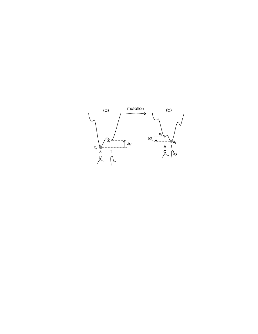
Figure 1: Schematic representations of the molecular energy landscapes. (a) For the non-mutated molecule. (b) For the mutated molecule. Only the two lowest energy conformations, A (active) and I (inactive), are taken into account. Their 3D conformations are indicated symbolically. The shaded dots indicate the populations $\pi_{\mathrm{A}}$ and $\pi_{\mathrm{I}}$ at thermal equilibrium.

From the distributions of free energy differences and eq. (3), one infers the probability distributions $P_{\mathrm{e\,or\,G}}(\pi_{\mathrm{A}})$ of the population of conformer state A after a mutation using $P_{\mathrm{e\,or\,G}}(\pi_{\mathrm{A}})=P_{\mathrm{e\,or\,G}}(\delta G_{\mathrm{M}})\times|{\mathrm{d}}\delta G_{\mathrm{M}}/{\mathrm{d}}\pi_{\mathrm{A}}|$. For the Gaussian model, one obtains:

$$P_{\mathrm{G}}(\pi_{\mathrm{A}})=\frac{\exp\left[\frac{-\left(\ln\pi_{\mathrm{A}}-\ln(1-\pi_{\mathrm{A}})-\bar{g}\right)^{2}}{2g_{0}^{2}}\right]}{\sqrt{2\pi}g_{0}\pi_{\mathrm{A}}(1-\pi_{\mathrm{A}})}\,,$$ (4)

where $\bar{g}\equiv\overline{\delta G}/(RT)$, $g_{0}\equiv\delta G_{0}/(RT)$. The ratio $g_{0}$ of the scale of energy fluctuations and of the thermal energy appears frequently in the study of the anomalous kinetics of disordered systems. For the exponential model, one obtains:

$$P_{\mathrm{e}}(\pi_{\mathrm{A}})=\frac{e^{-\bar{g}/g_{0}}}{2g_{0}\pi_{\mathrm{A}}^{1-1/g_{0}}(1-\pi_{\mathrm{A}})^{1+1/g_{0}}}\;\mathrm{for}\;\pi_{\mathrm{A}}\leq\pi_{\mathrm{m}},$$ (5a)

$$P_{\mathrm{e}}(\pi_{\mathrm{A}})=\frac{e^{+\bar{g}/g_{0}}}{2g_{0}\pi_{\mathrm{A}}^{1+1/g_{0}}(1-\pi_{\mathrm{A}})^{1-1/g_{0}}}\;\mathrm{for}\;\pi_{\mathrm{A}}\geq\pi_{\mathrm{m}},$$ (5b)

with the same definitions for $\bar{g}$ and $g_{0}$, and $\pi_{\mathrm{m}}\equiv\left(1+e^{-\bar{g}}\right)^{-1}$ (median population of A). Note that changing $\bar{g}$ into $-\bar{g}$ is equivalent to performing a symmetry on $P_{\mathrm{e\,or\,G}}(\pi_{\mathrm{A}})$ by replacing $\pi_{\mathrm{A}}$ by $1-\pi_{\mathrm{A}}$.

III Types of distributions

To analyze the different types of population distributions, we focus for definiteness on the Gaussian model. A qualitatively similar behavior is obtained for the exponential model. Figure 2 represents examples of $P_{\mathrm{G}}(\pi_{\mathrm{A}})$ for the Gaussian model with $\bar{g}=-1$ and various $g_{0}$’s. The negative value of $\bar{g}$ implies that A is on average less stable than I, and hence that $\pi_{\mathrm{A}}$ is predominantly less than 50%. For small $g_{0}$, the distribution $P_{\mathrm{G}}(\pi_{\mathrm{A}})$ is narrow since the width $\delta G_{0}$ of the free energy distribution is small compared to $RT$ so that there are only small fluctuations of population around the most probable value. When the energy broadness $g_{0}$ increases, the single narrow peak first broadens till, when $g_{0}\gtrsim 1.976$ it splits into two peaks, close respectively to $\pi_{\mathrm{A}}=0$ and to $\pi_{\mathrm{A}}=1$. The broad character of $P_{\mathrm{G}}(\pi_{\mathrm{A}})$ can be intuitively understood as a consequence of the non linear dependence of $\pi_{\mathrm{A}}$ on $\delta G_{\mathrm{M}}$. Thus, when the fluctuations of $\delta G_{\mathrm{M}}$ are larger than $RT$, i.e., when $g_{0}\gtrsim 1$, the quasi exponential dependence of $\pi_{\mathrm{A}}$ on $\delta G_{\mathrm{M}}$ (eq. (3)) non linearly magnifies $\delta G_{\mathrm{M}}$ fluctuations to yield a broad $\pi_{\mathrm{A}}$ distribution, even if $\delta G_{\mathrm{M}}$ fluctuations are relatively small compared to the mean $\overline{\delta G}$. A similar mechanism is at work for tunneling in disordered systems Costa et al. (2002); Romeo et al. (2003).

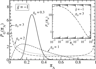
Figure 2: Distributions $P_{\mathrm{G}}(\pi_{\mathrm{A}})$ of shape populations of mutated molecules for $\bar{g}=-1$. They are narrow and single peaked for small enough $g_{0}$ and broad and double peaked for large enough $g_{0}$. The transition from one to two peaks occurs at $g_{0}\simeq 1.976$ in agreement with eq. (6). Inset: logarithmic plot of $P_{\mathrm{G}}(\pi_{\mathrm{A}})$ for $g_{0}=3$ showing the broad character of the small $\pi_{\mathrm{A}}$ peak.

A global view of the possible shapes of $P_{\mathrm{G}}(\pi_{\mathrm{A}})$ is given in figure 3. For any given $\bar{g}$, when increasing $g_{0}$ starting from 0, the single narrow peak of $P_{\mathrm{G}}(\pi_{\mathrm{A}})$ first broadens then it splits into two peaks when $\bar{g}=\bar{g}_{\mathrm{sign}(\bar{g})}(g_{0})$ with

$$\bar{g}_{\pm}(g_{0})\equiv\pm\left[g_{0}\sqrt{g_{0}^{2}-2}+\ln\left(\frac{g_{0}-\sqrt{g_{0}^{2}-2}}{g_{0}+\sqrt{g_{0}^{2}-2}}\right)\right].$$ (6)

(This expression results from a lengthy but straightforward study of $P_{\mathrm{G}}(\pi_{\mathrm{A}})$.) When $g_{0}$ increases further, these two peaks get closer to $\pi_{\mathrm{A}}=0$ and to $\pi_{\mathrm{A}}=1$ while acquiring significant tails (see section VII). For any given $g_{0}$, increasing $\bar{g}$ roughly amounts to moving the populations $\pi_{\mathrm{A}}$ towards larger values as expected since larger $\bar{g}$’s correspond to stabler states A. However, distinct behaviours arise depending on $g_{0}$. If $g_{0}<\sqrt{2}$, whatever the value of $\bar{g}$, the distribution $P_{\mathrm{G}}(\pi_{\mathrm{A}})$ is always sufficiently narrow to present a single peak. If $g_{0}>\sqrt{2}$, the distribution $P_{\mathrm{G}}(\pi_{\mathrm{A}})$ is sufficiently broad to have two peaks when, furthermore, the distribution is not too asymmetric, which occurs for $\bar{g}\in[\bar{g}_{-}(g_{0}),\bar{g}_{+}(g_{0})]$. In short, depending on $\bar{g}=\delta\bar{G}/RT$, which characterizes mainly the peak(s) position, and on $g_{0}=G_{0}/RT$, which characterizes mainly the distribution broadness, the distributions $P_{\mathrm{G}}(\pi_{\mathrm{A}})$ are either unimodal or bimodal, either broad or narrow. This variety of behaviors is reminiscent of beta distributions.

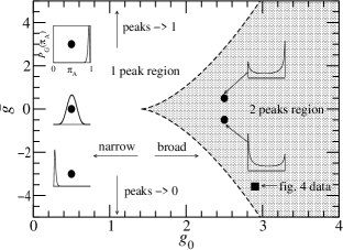
Figure 3: Possible shapes of $P_{\mathrm{G}}(\pi_{\mathrm{A}})$. The shaded area indicates the two-peaks region. The dashed line gives the transition from one to two peaks (cf. eq. (6)). Insets show examples of $P_{\mathrm{G}}(\pi_{\mathrm{A}})$ corresponding to the $g_{0}$ and $\bar{g}$ indicated by the black dots ($P_{\mathrm{G}}$’s not to scale). The black square corresponds to the fit of figure 4 data.

IV From shape populations to catalytic activities

Up to now, we have discussed the distribution $P(\pi_{\mathrm{A}})$ of the population of a shape A that is functionally active. However, as far as it concerns biopolymers with enzymatic functions, what is usually measured is a chemical activity $a$, i.e., the product of a reaction rate $k$ for the conformer A by the population $\pi_{\mathrm{A}}$ of this conformer. The reaction rates are given by the Arrhenius law $k=k_{0}e^{-E_{\mathrm{a}}/RT}$ where $k_{0}$ is a constant and $E_{\mathrm{a}}$ is the activation energy. Thus, the chemical activity writes, using eq. (3):

$$a=k_{0}e^{-E_{\mathrm{a}}/RT}\frac{1}{1+e^{-\delta G_{\mathrm{M}}/RT}}.$$ (7)

Random mutations may induce random modifications of $E_{\mathrm{a}}$, $\delta G_{\mathrm{M}}$ or both. Fluctuations of $\delta G_{\mathrm{M}}$ have been treated above. One can introduce fluctuations of $E_{\mathrm{a}}$ in the same way. We do not do it here in details but present only the general trends.

The effects of adding an activation energy distribution in addition to the free energy difference distribution are twofold. For small activities, the distribution $P(a)$ of chemical activities is similar to the small $P(\pi_{\mathrm{A}})$ peak at small $\pi_{\mathrm{A}}$. Indeed, the reaction rate $k$ depends exponentially on $E_{\mathrm{a}}$, just as the population $\pi_{\mathrm{A}}$ depends exponentially on $\delta G_{\mathrm{M}}$ when $\pi_{\mathrm{A}}\ll 1$. Moreover, the product of two broadly distributed random variables is also broadly distributed with a shape similar to the one of $P(\pi_{\mathrm{A}})$. For large activities, on the other hand, $\pi_{\mathrm{A}}$ and $k$ behave differently because $\pi_{\mathrm{A}}$ is bounded by 1 while $k$ is unbounded. Thus, if the $k$ distribution is broad enough, the distribution of $a$ at large $a$ may exhibit a broadened structure compared to the $\pi_{\mathrm{A}}\simeq 1$ peak of $P(\pi_{\mathrm{A}})$.

In summary, the distribution of chemical activities $P(a)$ is similar to the distribution of shape populations $P(\pi_{\mathrm{A}})$ when $P(\pi_{\mathrm{A}})$ presents a large $\pi_{\mathrm{A}}\simeq 0$ peak (conditions for this to occur are explicited in section VI). Thus, by observing the shape of the $a\simeq 0$ peak in the activity distribution $P(a)$, one does not easily distinguish between activation energy dispersion, which affects $k$, and free energy difference dispersion, which affects $\pi_{\mathrm{A}}$. On the other hand, at large $a$, $P(a)$ is differently influenced by activation energy dispersion and by free energy difference dispersion. The available experimental data (see section V) enables us to analyze precisely $P(a)$ at small activities but not at large activities. Thus, for practical purposes, it is not meaningful in this paper to consider a distribution of activation energies on top of a distribution of free energy differences. In the sequel, we will thus do as if only the distribution of free energies was involved, stressing that similar effects can be obtained from a distribution of activation energies.

V Analysis of experimental data

Comparison of the theoretical distributions of eq. (5) and eq. (4) with experimental data enables us to test the relevance of the proposed model. We have analyzed the measurements of the catalytic activities of a set of 157 mutants derived from a self-splicing group I ribozyme, a catalytic RNA molecule Couture et al. (1990) (out of the 345 mutants generated in Couture et al. (1990), we only considered the 157 ones with single point mutations). The original ”wild-type” molecule is formed of a conserved catalytic core that catalyzes the cleavage of another part of the molecule considered as the substrate. The set of mutants is derived from the original ribozyme by performing systematically all single point mutations of the catalytic core, i.e., of the part of the molecule that influences most the catalytic activity. Nucleotides out of the core, that in general influence less the catalytic activity, are left unmutated. Thus, in our framework, this set of mutants can be seen as biased towards deleterious mutations. Indeed, mutations of the quasi optimized core are likely to lead to much less active mutants, while mutations of remote parts are likely to leave the activity essentially unchanged. If all parts of the molecule had been mutated, more neutral or quasi neutral mutations would have been obtained. Another point of view, which we adopt here is to consider the catalytic core as a molecule in itself, on which all possible single point mutations have been performed.

The 157 measured activities are used to calculate a population distribution with inhomogenous binning (cf. broad distribution). Two bins required special treament: the smallest bin, centered in 0.5%, contains 40 mutants with non measurably small activities ($<1\%$ of the original activity); the largest bin, centered in 95%, contains the 6 mutants with activities larger than 90% of the original ’wild’ RNA activity (the largest measured mutant activity is 140%). These two points, whose abscissae are arbitrary within an interval, are not essential for the obtained results. At last, as very few mutants have activities larger than the wild-type ribozyme, the proportionality constant between activity and population is set by matching a population $\pi_{\mathrm{A}}=1$ to the activity of the wild-type ribozyme.

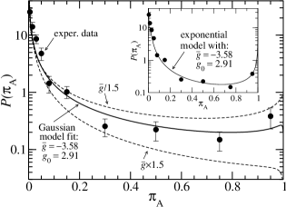
Figure 4: Analysis of an experimental distribution of activities. Experimental data are derived from Couture et al. (1990). Error bars give the one standard deviation statistical uncertainty. The solid line is a two parameter fit ($\bar{g}$, $g_{0}$) to the model of Gaussian energy distribution. The dashed lines correspond to the same $g_{0}$ and modified $\bar{g}$’s, which enables to estimate the uncertainty on $\bar{g}$. Inset: comparison of the data to the model of exponential energy distribution ($g_{0}$ and $\bar{g}$ are not fitted again but taken from the Gaussian model fit).

The obtained distribution (see figure 4) has a large peak in $\pi_{\mathrm{A}}\simeq 0$, indicating that most mutations are deleterious, with a long tail at larger activities and a possible smaller peak in $\pi_{\mathrm{A}}\simeq 1$. This non trivial shape is well fitted by the Gaussian model of eq. (4) with $\bar{g}=-3.6$ and $g_{0}=2.9$ (the uncertainty on these parameters is about 50%, see dashed lines in figure 4). One infers $\overline{\delta G}\simeq-2.1$ kcal/mol and $\delta G_{0}\simeq 1.7$ kcal/mol ($T=300$ K). The order of magnitude of these values is compatible with thermodynamic measurements performed on similar systems Jaeger et al. (1993, 1994); Brion and Westhof (1997); Brion et al. (1999). This confirms the plausibility of the proposed approach. The inset of figure 4 shows the population distribution in the exponential model with $\bar{g}$ and $g_{0}$ values taken from the Gaussian fit. The agreement with the experimental data is also quite good. Thus, the proposed approach soundly does not strongly depend on the yet unknown shape details of the energy distribution. Finally, one can estimate the broad character of the activity distribution from the statistical analysis of the experimental data. Indeed, according, e.g., to the Gaussian model fit, the typical, most probable, population $\pi_{\mathrm{A}}$ is found to be $\simeq 6\times 10^{-6}$ while the mean population is $\simeq 0.15$. Thus, the activity distribution spans more than four orders of magnitude.

VI Coarse graining description: all or none features

The variation of activity of a biopolymer upon mutation is often described as an ‘all or none’ process: mutations are considered either as neutral (the mutant retains fully its activity and $\pi_{\mathrm{A}}\simeq 100$ %) or as lethal (the mutant loses completely its activity and $\pi_{\mathrm{A}}\simeq 0$ %). Satisfactorily, a coarse graining description of the proposed statistical models exhibits such all or none regimes for appropriate $(\bar{g},g_{0})$ values, as well as other regimes.

To obtain a quantitative coarse graining description, we define the mutants with ’no’ activity as those with population that has less than $12\ \%$ ($\simeq\pi_{\mathrm{A}}(\delta G_{\mathrm{M}}=-2RT)$) in the A shape. Their weight is

$$w_{0}=\int_{0}^{12\%}\!\!\!\!P_{\mathrm{e\,or\,G}}(\pi_{\mathrm{A}}){\mathrm{d}}\pi_{\mathrm{A}}=\int_{-\infty}^{-2RT}\!\!\!\!P_{\mathrm{e\,or\,G}}(\delta G)\ {\mathrm{d}}\delta G.$$ (8)

Similarly, the mutants with ‘full’, respectively ’intermediate’, activity are defined as those with $\pi_{\mathrm{A}}\geq 88\%$, respectively $12\%\leq\pi_{\mathrm{A}}\leq 88\%$, and their weight is $w_{100}=\int_{2RT}^{\infty}P_{\mathrm{e\,or\,G}}(\delta G)\ {\mathrm{d}}\delta G$, respectively $w_{\mathrm{i}}=\int_{-2RT}^{+2RT}P_{\mathrm{e\,or\,G}}(\delta G)\ {\mathrm{d}}\delta G$. Taking for definiteness the Gaussian model leads to

$$w_{0}=\Phi\left(-\frac{2}{g_{0}}-\frac{\bar{g}}{g_{0}}\right)$$ (9)

where $\Phi(u)=\int_{-\infty}^{u}e^{-t^{2}/2}{\mathrm{d}}t/\sqrt{2\pi}$ is the distribution function of the normal distribution. Similarly, one has $w_{\mathrm{i}}=\Phi[(2-\bar{g})/g_{0}]-\Phi[-(2+\bar{g})/g_{0}]$ and $w_{100}=1-\Phi[(2-\bar{g})/g_{0}]$. Approximate expressions for $\Phi(u)$ ($\Phi(u)\simeq-e^{-u^{2}/2}/(\sqrt{2\pi}u)$ for $u\ll-1$, $\Phi(u)\simeq 1/2+u/\sqrt{2\pi}$ for $|u|\ll 1$ and $\Phi(u)\simeq 1-e^{-u^{2}/2}/(\sqrt{2\pi}u)$ for $u\gg 1$) give the regimes in which each weight $w$ is negligible ($w\ll 1$), dominant ($1-w\ll 1$) or in between. For instance, $w_{0}$ is negligible for $\bar{g}>g_{0}-2$, dominant for $\bar{g}<-g_{0}-2$ and intermediate for $-g_{0}-2<\bar{g}<g_{0}-2$. These inequalities indicate the transition from one regime to another. To be strictly in one regime requires typically that $\bar{g}/g_{0}$ is larger or greater than 1 from the corresponding criterion, e.g., $w_{0}$ is strictly negligible when $\bar{g}/g_{0}>1+(g_{0}-2)/g_{0}$ The transitions from one regime to another one are in general exponentially fast (solid lines in figure 5). However, in the region ($g_{0}>2$, $|\bar{g}|<g_{0}-2$), the transitions from one regime to another one are smooth (dashed lines in figure 5) since, in this region, the weights vary slowly, e.g., $w_{\mathrm{i}}\simeq 4/(g_{0}\sqrt{2\pi})$.

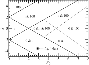
Figure 5: Coarse graining features of the population distribution $P_{\mathrm{G}}(\pi_{\mathrm{A}})$ in the Gaussian model. In each region, the population ranges dominating the distribution have been indicated ($0$ for $\pi_{\mathrm{A}}\leq 12\%$, i for $12\%\leq\pi_{\mathrm{A}}\leq 88\%$ and 100 for $\pi_{\mathrm{A}}\geq 88\%$).

The resulting coarse graining classification of $P_{\mathrm{G}}(\pi_{\mathrm{A}})$ is represented in figure 5. The ‘all or none’ behaviour, denoted ‘0 & 100’, appears in the region $g_{0}\gtrsim 6/\sqrt{\pi/2}$ and $|\bar{g}|\lesssim\sqrt{\pi/2}g_{0}-6$ as the result of a large dispersion of energy differences associated to a moderate average energy difference. We note that all possible types of distributions are actually present in this model: probabilities concentrated at small, intermediate or large values (0, i or 100); probabilities spread over both small and intermediate (0 & i), both small and large (0 & 100, all or none) or both intermediate and large (i & 100) values; probabilities spread over small, intermediate and large values at the same time (0 & i & 100). The coarse graining classification of figure 5 complements the number of peaks classification of figure 3 without overlapping it. Indeed, there exist parameters $g_{0}$ and $\bar{g}$ for which, e.g., two peaks coexist but one of these peaks has a negligible weight. Thus the presence of a peak is not automatically associated to a large weight in the region of this peak.

VII Zooming in the $\pi_{\mathrm{A}}\simeq 0$ peak: long tails

To go beyond the coarse graining description, we zoom in the $\pi_{\mathrm{A}}\simeq 0$ peak. As shown in the inset of figure 3, the small activities, labelled as ‘no activity’ in a coarse graining description, actually consist of non zero activities with values scanning several orders of magnitude. This can be analyzed quantitatively, e.g., in the Gaussian model. For $\pi_{\mathrm{A}}\simeq 0$, the activity distribution given by eq. (4) is quasi lognormal:

$$P_{\mathrm{G}}(\pi_{\mathrm{A}})\simeq\frac{1}{\sqrt{2\pi}g_{0}\pi_{\mathrm{A}}}\exp\left[\frac{-(\ln\pi_{\mathrm{A}}-\bar{g})^{2}}{2g_{0}^{2}}\right]\ .$$ (10)

Thus, $P_{\mathrm{G}}(\pi_{\mathrm{A}})$ has as a power law like behavior Romeo et al. (2003); Montroll and Shlesinger (1983):

$$P_{\mathrm{G}}(\pi_{\mathrm{A}})\simeq\frac{1}{\sqrt{2\pi}g_{0}\pi_{\mathrm{A}}}\quad\mathrm{for}\quad e^{\bar{g}-\sqrt{2}g_{0}}\lesssim\pi_{\mathrm{A}}\lesssim e^{\bar{g}+\sqrt{2}g_{0}},$$ (11)

in the vicinity of the lognormal median $e^{\bar{g}}$. This corresponds to an extremely long tailed distribution, since $1/\pi_{\mathrm{A}}$ is not even normalizable. It presents the peculiarity that, for $a$ and $a+1$ belonging to $[\bar{g}-\sqrt{2}g_{0},\bar{g}+\sqrt{2}g_{0}]$, the probability to obtain a population $\pi_{\mathrm{A}}$ of a given order of magnitude $a$, i.e., $\pi_{\mathrm{A}}\in[e^{a},e^{a+1}]$, does not depend on the considered ordered of magnitude $a$, since

$$\int_{e^{a}}^{e^{a+1}}P_{\mathrm{G}}(\pi_{\mathrm{A}}){\mathrm{d}}\pi_{\mathrm{A}}\simeq\mathrm{const}.$$ (12)

Thus, if a living organism has to adapt the chemical activity of one of its biopolymer constituents, it can explore several order of magnitude of activity by only few mutations within the biopolymer. The activity changes mimic a Lévy flight Bouchaud and Georges (1990) as revealed, e.g., by the experimental data in Schultes and Bartel (2000). The large activity changes will raise self-averaging issues Romeo et al. (2003) that will add up to those generated by correlations along evolutionary paths Bastolla et al. (2002)

Three broadness regimes corresponding to three evolutionary regimes can be distinguished. If $g_{0}$ is very large, the mutant activities span a very large range. This regime might be globally lethal because, in most cases, the mutant activity will be either too low or too large to be biologically useful. However, under conditions of intense stress, the large variability might allow the system to evolve radically. With $g_{0}=10$, for instance, the activity range covers typically 12 orders of magnitude from $10^{-6}e^{\bar{g}}$ to $10^{6}e^{\bar{g}}$ (see eq. (11)). If $g_{0}$ is moderately large, the mutant activities span just a few orders of magnitude. This regime is broad enough to permit significant changes, but not too broad to avoid producing too many lethal changes. With $g_{0}=3$, for instance, the activity range covers typically $3-4$ orders of magnitude from $10^{-1.8}e^{\bar{g}}$ to $10^{1.8}e^{\bar{g}}$. If $g_{0}$ is small, the lognormal distribution peak can be approximated by a Gaussian Romeo et al. (2003)

$$P_{\mathrm{G}}(\pi_{\mathrm{A}})\simeq\frac{1}{\sqrt{2\pi}g_{0}e^{\bar{g}}}\ \exp\left[\frac{-(\pi_{\mathrm{A}}-e^{\bar{g}})^{2}}{2(g_{0}e^{\bar{g}})^{2}}\right].$$ (13)

The distribution is now narrow and the ranges of values is typically $[e^{\bar{g}}(1-2g_{0}),e^{\bar{g}}(1+2g_{0})]$. This type of distribution is not adapted for producing large changes, but rather for performing fine tuning optimization. With $g_{0}=0.1$, for instance, the activity range covers only $\pm 20\%$ around $e^{\bar{g}}$.

We remark that the group I ribozyme which we have analyzed corresponds to $g_{0}\simeq 2.9$, right in the critical regime of moderately large $g_{0}$. One can guess from experimental studies of other biopolymers or from chemical considerations that most biopolymers will fall in this range since $\delta G_{0}$ is typically on the order of a few kilocalories while $RT$ is $\simeq 0.6$ kcal (Note that $\delta G_{0}$ corresponds to the free energy change between the biopolymer native 3D state and an unfolded state, in which the biopolymer has lost its three-dimensional shape but not its full secondary structure). It would be interesting to perform further statistical data analysis to see how, e.g., the available protein mutagenesis studies fit with our present model.

The energy statistics associated mutations is likely to be determined at gross scale by the basic biophysics of the molecules involved. This fixes a range for $\delta G_{0}$. It is nonetheless plausible and suggested by our discussion that there is an evolutionary preferred type of activity distribution, and hence of sequences, that may imply a fine tuning of $g_{0}=\delta G_{0}/RT$ within the constraints on $\delta G_{0}$ coming from biophysics (see figure 6) so that each mutation typically generates a significant, but not systematically lethal, activity change. If one considers that the activity changes must cover between, say, one and seven orders of magnitude, then the allowed $g_{0}$ range is $1-6$ (see eq. (11)).

To answer the question whether the energy statistics is solely dictated by molecular biophysics or whether it is also influenced by evolutionary requirements, one may compare the energy statistics of molecules from different thermal environments. The conservation of the $\delta G_{0}$ range across psychrophilic and thermophilic molecules would stress the domination of biophysics factors. Note that our model would then imply different stochastic evolutionary dynamics, through the width of the activity distribution, for psychrophilic and thermophilic environments. Conversely, the conservation of $g_{0}$ would reveal the importance of evolutionary requirements.

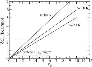
Figure 6: Free energy dispersion $\delta G_{0}$ as a function of $g_{0}$ for different temperatures $T$. The upper and lower temperature limits for life are, respectively, $\simeq 121^{\circ}$ C and $\simeq~{}-20^{\circ}$ C. Depending on whether the energy statistics is determined by the biophysics or by evolutionary requirements, the range of either $\delta G_{0}$ or of $g_{0}$ is fixed (see for example the dashed lines). Evolutionary requirements suggest $1\lesssim g_{0}\lesssim 6$.

VIII Conclusions

In this paper, we have presented a model for the distribution of biopolymer activities resulting from mutations of a given sequence. The model is characterized by the statistics of the energy differences between active conformations and inactive conformations. A similar model would be obtained by considering the statistics of activation energies. The model fits the measured activity distribution of a ribozyme with energy parameters in the physically appropriate range. It is also able to reproduce commonly observed behaviours such as all or none.

Importantly, the peak of small activities exhibits three distinct types depending on the broadness of the distribution of energy differences. Real biopolymers are in a critical regime allowing the exploration of different ranges of activities in a few mutations without being too often lethal. This critical regime seems the most favorable evolutionary regime and could be the statistical engine allowing molecular evolution. Thus the present work supports the idea that, for evolution to take place, the temperature and the physico-chemistry dictating the free energy scales of biopolymers must obey a certain ratio. At last, it suggests that, by looking at small variations of this ratio, one might be able to classify biopolymers. One expects, for instance, that biopolymer sequences that are locked in a shape with a specific function, will have smaller $g_{0}$ than rapidly evolving biopolymers sequences that could acquire new functions by undergoing major structural changes. Thus, at the origin of life or during rapidly evolving punctuations, biopolymers with larger $g_{0}$ than those characterizing highly optimized, modern RNA and protein molecules, could have contributed to the emergence of novel phenotypes, leading thus to an increase of complexity.

References

- Fontana (2002) W. Fontana, BioEssays 24, 1164 (2002).
- Kimura (1968) M. Kimura, Nature 217, 624 (1968).
- Kimura (1993) M. Kimura, The Neutral Theory of Molecular Evolution (Cambridge University Press, Cambridge, 1993).
- Schuster et al. (1994) P. Schuster, W. Fontana, P. F. Stadler, and I. L. Hofacker, Proc. R. Soc. London B 255, 279 (1994).
- Perelson and Oster (1979) A. S. Perelson and G. F. Oster, J. Theor. Biol. 81, 645 (1979).
- Schultes and Bartel (2000) E. A. Schultes and D. P. Bartel, Science 289, 448 (2000).
- Fontana and Schuster (1998) W. Fontana and P. Schuster, Science 280, 1451 (1998).
- Ancel and Fontana (2000) L. W. Ancel and W. Fontana, J. Exp. Zoology 288, 242 (2000).
- Shlesinger et al. (1995) M. F. Shlesinger, G. M. Zaslavsky, and U. Frisch, eds., Lévy Flights and Related Topics in Physics, vol. 450 of Lecture Notes in Physics (Springer-Verlag, Berlin, 1995).
- Kutner et al. (1999) R. Kutner, A. Pȩkalski, and K. Sznajd-Weron, eds., Anomalous diffusion: from basics to applications, Proceedings of the XIth Max Born Symposium Held at La̧dek Zdrój, Poland, 20-27 May 1998 (Springer-Verlag, Berlin, 1999).
- Bardou et al. (2002) F. Bardou, J. P. Bouchaud, A. Aspect, and C. Cohen-Tannoudji, Lévy Statistics and Laser Cooling (Cambridge University Press, Cambridge, 2002).
- Elredge and Gould (1972) N. Elredge and S. J. Gould, in Models in Paleobiology, edited by T. J. M. Schopf (Freeman Cooper & Co, San Francisco, 1972), pp. 82–115.
- Doliwa and Heuer (2003) B. Doliwa and A. Heuer, Energy barriers and activated dynamics in a supercooled lennard-jones liquid (2003).
- Costa et al. (2002) V. D. Costa, M. Romeo, and F. Bardou, J. Magn. Magn. Mater. 258-259, 90 (2002).
- Romeo et al. (2003) M. Romeo, V. D. Costa, and F. Bardou, Eur. Phys. J. B 32, 513 (2003).
- Couture et al. (1990) S. Couture, A. D. Ellington, A. S. Gerber, J. M. Cherry, J. A. Doudna, R. Green, M. Hanna, U. Pace, J. Rajagopal, and J. W. Szostak, J. Mol. Biol. 215, 345 (1990).
- Jaeger et al. (1993) L. Jaeger, E. Westhof, and F. Michel, J. Mol. Biol. 234, 331 (1993).
- Jaeger et al. (1994) L. Jaeger, F. Michel, and E. Westhof, J. Mol. Biol. 236, 1271 (1994).
- Brion and Westhof (1997) P. Brion and E. Westhof, Annu. Rev. Biophys. Biomol. Struct. 26, 113 (1997).
- Brion et al. (1999) P. Brion, F. Michel, R. Schroeder, and E. Westhof, Nucleic Acid Res. 27, 2494 (1999).
- Montroll and Shlesinger (1983) E. W. Montroll and M. F. Shlesinger, J. Stat. Phys. 32, 209 (1983).
- Bouchaud and Georges (1990) J.-P. Bouchaud and A. Georges, Phys. Rep. 195, 127 (1990).
- Bastolla et al. (2002) U. Bastolla, M. Porto, H. E. Roman, and M. Vendruscolo, Phys. Rev. Lett. 89, 208101.1 (2002).
- Onuchic et al. (1997) J. N. Onuchic, Z. LutheySchulten, and P. G. Wolynes, Annu. Rev. Phys. Chem. 48, 545 (1997).