Primary population of antiprotonic helium states

Abstract

A full quantum mechanical calculation of partial cross-sections leading to different final states of antiprotonic helium atom was performed. Calculations were carried out for a wide range of antiprotonic helium states and incident (lab) energies of the antiproton.

I Introduction

One of the most impressive success stories of the last decade in few-body physics is the high precision experimental and theoretical studies of long lived states in antiprotonic helium (for an overview see Yamazaki et al. (2002)). While the energy levels have been both measured and calculated to an extreme precision, allowing even for improvement of numerical values of fundamental physical constants, some other relevant properties of these states were studied with considerably less accuracy. Among these is the formation probability of different metastable states $(J,v)$ in the capture reaction

$$\bar{p}\,+\,^{4}He\longrightarrow(^{4}He^{+}\,\bar{p})_{Jv}+e^{-}.$$ (1)

The existing calculations of the capture rates of slow antiprotons in $He$ Korenman (1996, 2001); Cohen (2000) are based on classical or semiclassical approaches and they mainly address the reproduction of the overall fraction (3%) of delayed annihilation events. Recent experimental results from the ASACUSA project Hori et al. (2002), however, yield some information on individual populations of different metastable states, and our aim is to perform a fully quantum mechanical calculation of the formation probability of different states in the capture reaction.

II Calculation Method

The exact solution of the quantum mechanical four-body problem, underlying the reaction (1) is far beyond the scope of this work, and probably also of presently available calculational possibilities. Still, we want to make a full quantum mechanical, though approximate, calculation of the above process. Full is meant in the sense that all degrees of freedom are taken explicitly into account, all the wave functions we use, are true four-body states.

The simplest way to realize this idea is to use the plane wave Born approximation which amounts to replacing in the transition matrix element the exact scattering wave function $\Psi_{i}^{+}$ by its initial state $\Phi_{i}$ which preceded the collision.

$$T_{fi}=\langle\Phi_{f}|V_{f}|\Psi_{i}^{+}\rangle\approx\langle\Phi_{f}|V_{f}|\Phi_{i}\rangle.$$ (2)

In our case the initial and final wave functions were taken in the form:

$$\Phi^{i}_{He,\,{\bf K}_{i}}({\bf r}_{1},{\bf r}_{2},{\bf R}) = \Phi_{He}({\bf r}_{1},{\bf r}_{2})\,\frac{1}{(2\pi)^{3/2}}\,e^{i{\bf K}_{i}{\bf R}}$$

$$\Phi^{f}_{Jv,\,{\bf K}_{f}}(\mbox{\boldmath{$\rho$}}_{1},\mbox{\boldmath{$\rho$}}_{2},{\bf R}) = \Phi_{Jv}(\mbox{\boldmath{$\rho$}}_{1},{\bf R})\,\frac{1}{(2\pi)^{3/2}}\,e^{i{\bf K}_{f}\mbox{\boldmath{$\rho$}}_{2}}$$

where ${\bf r}_{i}$ are the vectors pointing from helium to the $i$-th electron, ${\bf R}$ is the vector between $He$ and $\bar{p}$, while $\mbox{\boldmath{$\rho$}}_{i}$ are the Jacobian vectors connecting the electrons with the center of mass of the $He-\bar{p}$ system. For the $He$ the ground state wave function we used the simplest effective charge hydrogen-like ansatz Bethe and Salpeter (1957)

$$\Phi_{He}(\bf{r}_{1},\bf{r}_{2})=N\,\exp{(-\sigma(r_{1}+r_{2}))}.$$ (3)

For the antiprotonic helium wave function we used the Born-Oppenheimer form Shimamura (1992); Révai and Kruppa (1998), which correctly reflects the main features of the final state:

$$\Phi_{Jv}(\mbox{\boldmath{$\rho$}},{\bf R})=\frac{\chi_{Jv}(R)}{R}\,Y_{JM}(\hat{R})\phi_{1\sigma}(\mbox{\boldmath{$\rho$}};{\bf R})$$ (4)

where $\phi_{1\sigma}(\mbox{\boldmath{$\rho$}};{\bf R})$ is a ground state two-center wave function, describing the electron motion in the field of $He$ and $\bar{p}$ separated by a fixed distance $R$, while $\chi_{Jv}(R)$ is the heavy-particle relative motion wave function corresponding to $({}^{4}He\,\bar{p}\;e^{-})$ angular momentum $J$ and ”vibrational” quantum number $v$. The transition potential $V_{f}$ is obviously

$$V_{f}=-\,\frac{2}{{\bf r}_{2}}+\frac{1}{|{\bf r}_{1}-{\bf R}|}+\frac{1}{|{\bf r}_{1}-{\bf r}_{2}|}_{\,.}$$

The partial cross-section leading to a certain antiprotonic helium state $(Jv)$ can be written as

$$\sigma_{Jv}=(2\pi)^{4}\,{K_{f}\over K_{i}}\,\mu_{i}\,\mu_{f}\int d\Omega_{{\bf K}_{f}}\left|\langle\Phi^{f}_{Jv,{\bf K}_{f}}|V_{f}|\,\Phi^{i}_{He,{\bf K}_{i}}\rangle\right|^{\,2}_{\,.}$$ (5)

The angular integrations occurring in the evaluation of Eq. (5) were carried out exactly, using angular moment algebra, while the 3-fold radial integrals were calculated numerically.

The general expression (5) for the cross-section leading to a specific state $(Jv)$ can be rewritten in terms of matrix element between angular momentum eigenstates as

$$\sigma_{Jv}=(2\pi)^{4}\,{K_{f}\over K_{i}}\,\mu_{i}\,\mu_{f}\sum_{\Lambda,l}(2\Lambda+1)\,|M_{J,l}^{\Lambda}|^{2}$$ (6)

with

$$M_{J,l}^{\Lambda}=\langle\,[\Phi_{Jv}\,\phi_{K_{f},l}(\mbox{\boldmath{$\rho$}}_{2})]_{M}^{\Lambda}\,|\,V_{f}\,|\,[\Phi_{He}\,\phi_{K_{i},\Lambda}({\bf R})]_{M}^{\Lambda}\,\rangle,$$ (7)

where $\phi_{K,l}({\bf r})$ denotes free states which definite angular momentum

$$\phi_{K,l}({\bf r})=\sqrt{\frac{2}{\pi}}\,j_{l}(Kr)Y_{lm}(\hat{r})$$

and $[\,\,\,]_{M}^{J}$ stands for vector coupling. Since the angular momentum of the $He$ ground state is zero, the total angular momentum $\Lambda$ of the incident side is carried by the antiproton. A given antiprotonic helium final state $Jv$ can be formed with different total angular momenta $\Lambda$ depending on the orbital momentum $l$ carried away by the emitted electron. Our calculations show, that only the values $l=0$ and $l=1$ give a non-negligible contribution to the sum in Eq. (6).

III Results and Discussion

We have calculated the partial population cross-sections $\sigma_{Jv}$ for states with angular momentum $J$ and energy $E_{Jv}$ in the interval $J=25-51$, $E_{Jv}=-(4.9-2.3)$ a.u. For these states all the energetically allowed transitions were calculated for incident antiproton energies in the range $5-30$ eV.

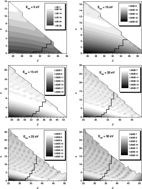
Figure 1: Overall distribution of calculated cross-sections over the quantum numbers $J$ and $v$ for different incident antiproton energies. The black line separates the short lived (on the left) and long lived states (on the right side of the line) of antiprotonic helium. All cross-sections are measured in units of $a_{0}^{2}$, $a_{0}$ being the atomic length unit.

Our overall results are presented on the contour plots of Fig. 1. The black line separates the regions of short-lived and long-lived states. The latter (on the right side of the line) are selected according to the usual criterium of Auger-electron orbital momentum $l_{Auger}\geq 4$.

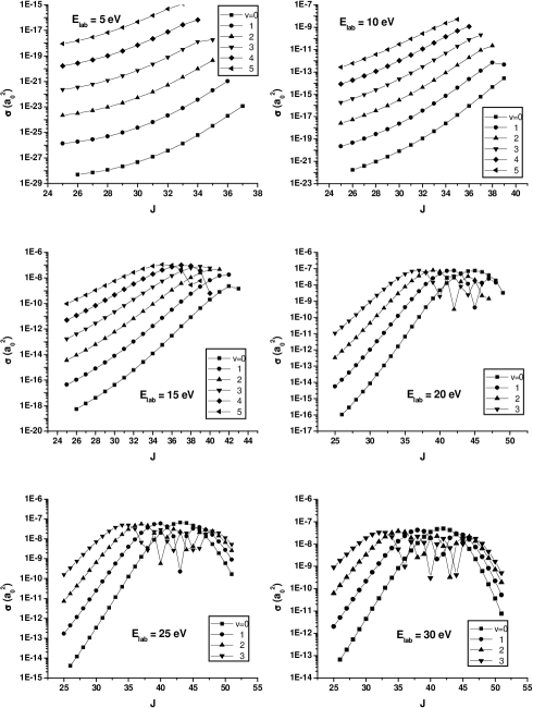
Figure 2: Cross-sections for the lowest few vibrational quantum numbers $v$ and different incident antiproton energies.

In Figs. 2–4 we tried to illustrate the dependence of certain selected cross-sections $\sigma_{Jv}(E)$ on their parameters. In Fig. 2 we displayed certain cross-sections for various incident energies as a function of antiprotonic helium angular momentum $J$, connecting points, which correspond to a certain vibrational quantum number $v$, while in Fig. 3 the connected points belong to the same principal quantum number $N=J+v+1$.

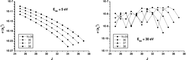
Figure 3: Examples of cross-sections with fixed $N$ in the ”smooth” and ”oscillatory” regime (see text).

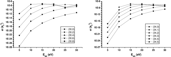
Figure 4: Dependence of selected cross-sections on incident antiproton energy.

Fig. 4 shows the dependence of a few cross-sections on the incident energy of antiproton.

A table, containing all our results, would not fit the size of this paper, however, it can be obtained from the authors upon request, or seen/downloaded at http://www.rmki.kfki.hu/~revai/table.pdf.

It is not easy to draw general conclusions about the relevant physics of antiproton capture from this bulk of data. There is, however, a conspicuous feature of our data, which deserve some consideration. In a certain region of antiprotonic helium states the dependence of the cross-sections on quantum numbers show a smooth, regular pattern, while with increasing excitation energy this behavior becomes irregular. On Fig. 1 this is seen as a transition from almost parallel stripes to an ”archipelago” type structure, while on Figs. 2–3 the smooth lines become oscillatory.

In order to reveal the origin of this phenomenon we looked into the structure of the matrix element in Eq (7) and found that its actual value is basically determined by the integration over $R$. We can rewrite (7) as

$$M_{J,l}^{\Lambda}\sim\int_{0}^{\infty}\chi_{Jv}(R)\,F(R)\,j_{\Lambda}(K_{i}R)\,R\,dR,$$ (8)

where $\chi_{Jv}(R)$ is the $He-\bar{p}$ relative motion wave function in the BO state ${Jv}$, $j_{\Lambda}(K_{i}R)$ is the spherical Bessel function of the incident $\bar{p}$, and $F(R)$ contains all rest: the potentials, the angular integrals, and the integrals over the electron coordinates. The expression (8) can be considered as a kind of ”radial, one-dimensional” Born approximation for the transition of the antiproton from the initial state $j_{\Lambda}(K_{i}R)$ to the final state $\chi_{Jv}(R)$ and $F(R)$ plays the role of the potential.

Figure 5: Parts of the integrand of Eq (8): $j_{\Lambda}(K_{i}R)$ (solid line), $\chi_{Jv}(R)$ (dashed line) and $F(R)$ (dotted line). For details see text.

Fig. 5 shows a few characteristic plots of $j_{\Lambda}(K_{i}R)$, $\chi_{Jv}(R)$, and $F(R)$. It can be seen, that $F(R)$ depends very weakly on the quantum numbers of the transition, thus its interpretation as ”transition potential” is not meaningless. The other essential conclusion from Fig. 5 is, that the value of the integral is basically determined by the overlap of two rapidly varying functions, $j_{\Lambda}(K_{i}R)$ and $\chi_{Jv}(R)$. While $\chi_{Jv}(R)$ is strongly localized with rapid decay in both directions $R\to\infty$ and $R\to 0$, $j_{\Lambda}(K_{i}R)$ is rapidly oscillating for large $R$ and — due to the high angular momentum $\Lambda$ — strongly decreasing in the direction $R\to 0$. For increasing $J$, $\chi_{Jv}$ slightly moves outwards, while increasing $v$ (the number of its nodes) makes it more and more oscillating. Increasing incident energy moves $j_{\Lambda}(K_{i}R)$ inwards. According to these general observations, the ”smooth regime” of the dependence of partial cross-sections on the energy and quantum numbers, corresponds to the situation, when only the ”outer” tail of $\chi_{Jv}(R)$ and the ”inner” tail of $j_{\Lambda}(K_{i}R)$ overlap. For increasing energy (incident or excitation) the oscillating parts of $\chi_{Jv}$ and $j_{\Lambda}$ might overlap leading to an irregular ”unpredictable” dependence on quantum numbers and incident energy.

This idea can be traced on the last two plots of Fig. 2. The $\chi_{Jv}(R)$ functions for a given $v$ are essentially of the same form, only with increasing $J$ they are pushed outwards into the region of oscillations of $j_{\Lambda}(K_{i}R)$. For the nodeless $v=0$ function this leads to a decrease of the integral in Eq. (8), while each node of the $v\neq 0$ functions produces a minimum in the cross-section when it penetrates into the region of non-vanishing $j_{\Lambda}(K_{i}R)$.

The three graphs on the right side of Fig. 5. demonstrate this phenomenon on the case of the 20 eV $v=1$ curve of Fig. 2. It can be seen, how the position of the node of $\chi_{Jv}(R)$ relative to the first peak of the $j_{\Lambda}(K_{i}R)$ Bessel-function brings about the minimum of the cross-section.

IV Conclusions

To our knowledge, this is the first calculation of the process (1) in which realistic final state wave functions were used. Due to this fact we think, that our results concerning the relative population of different final states might be reliable in spite of the poor treatment of the dynamics of the capture process. As for the absolute values of cross-sections, a more realistic dynamical treatment of the reaction (1) is probably inevitable.

The transition matrix elements are basically determined by the overlap of the BO function $\chi_{Jv}(R)$ and the incident Bessel function $j_{\Lambda}(K_{i}R)$ of the antiproton. All the rest can be incorporated into a potential-like function $F(R)$, which weakly depends on the quantum numbers of the transition. This feature will be probably preserved if a more realistic initial state wave function (both for the electrons and the antiproton) will be used.

The ”smooth” regime of the quantum number dependence of the partial cross-section allows to check the existing two ”thumb rules” Yamazaki et al. (2002); Shimamura (1992) for the most likely populated antiprotonic helium states. One of them states, that the mostly populated levels will have

$$N\sim\sqrt{\frac{M}{m}}\sim 37-38$$ (9)

while according to the other assumption, the maximum of the capture cross-section occurs for zero (or smallest possible) energy of the emitted electron and correspondingly for highest excitation energy. From our contour plots of Fig. 1 we can conclude, that the maximum cross-sections occur along a line, which can be approximated by

$$v(\sigma_{max})=a-b*J$$ (10)

with $a\sim 15-20$ and $b\sim 0.4-0.45$, depending on incident energy. This observation does not seem to confirm any of the ”thumb rules”.

As for comparison of our results with the recently obtained experimental data Hori et al. (2002), we would like to make two remarks. First, our calculations show, that the cross-sections strongly depend on incident antiproton energy. Since the energy distribution of the antiprotons before the capture is unknown, the direct comparison with the observed data is impossible. Secondly, any observed population data inevitably involve a certain time delay after formation and thus the effect of ”depopulation” due to collisional quenching. Since this effect is absent from our calculation, again, the comparison with experimental data is not obvious.