Dosimetry for radiocolloid therapy of cystic craniopharyngiomas

Abstract

The dosimetry for radiocolloid therapy of cystic craniopharyngiomas is investigated. Analytical calculations based on the Loevinger and the Berger formulae for electrons and photons, respectively, are compared with Monte Carlo simulations. The role of the material of which the colloid introduced inside the craniopharyngioma is made of as well as that forming the cyst wall is analyzed. It is found that the analytical approaches provide a very good description of the simulated data in the conditions where they can be applied (i.e., in the case of a uniform and infinite homogeneous medium). However, the consideration of the different materials and interfaces produces a strong reduction of the dose delivered to the cyst wall in relation to that predicted by the Loevinger and the Berger formulae.

I Introduction

Craniopharyngiomas are tumors showing an incidence of 3% for all tumors in adults and 6 to 10% of tumors in children Rub72 . Though histologically benign, they are effectively malignant because they usually appear in a situation which can affect to important organs such as hypothalamus, optic nerves or chiasms.

Treatment based on surgery followed (or not) by radiation therapy needs a total resection to guarantee a good chance of cure. However, a complete excision is rarely possible due to the vicinity of the organs mentioned above Sha79 .

Alternatively, the introduction of radioactive colloids into the cyst has been considered since the early 50’s Lek53 ; Wyc54 . Cyst wall constitutes the target volume and, as a consequence, $\beta$-emitters, as e.g. ³²P and ⁹⁰Y are the most adequate. Also $\beta\gamma$-emitters, as ¹⁸⁶Re and ¹⁹⁸Au, have been used, since $\gamma$-radiation allows to test the colloid distribution by obtaining a gamma camera image.

Cystic craniopharyngiomas are roughly spherical and the wall of the cyst presents a thickness between 1 and 3 mm. Once the radiocolloid is introduced inside the craniopharyngioma, part of it is attached to the inner surface of the cyst, while the rest appears to be distributed into the inner volume.

Dosimetry calculations for $\beta$ emitters have been carried out either on the base of the Loevinger formulation Loe56 (see e.g. NMT99 ) or by using the $\beta$ point kernels generated by Berger Ber71 (see e.g. Mcg86 ). In the case of $\beta\gamma$-emitters, the dose rates for photons have been evaluated following the approach of Berger Ber68 in terms of the build-up factors for the appropriate energies (see e.g. Mcg86 ).

In order to perform the dosimetry, because of the characteristic distribution of the radiocolloid, two extreme situations have been considered in practice NMT99 ; Mcg86 . The first one is the spherical shell source, where the emitter is supposed to be uniformly distributed in the inner surface of the cyst. The second one is the spherical volume source (SVS), which assumes the radionuclide uniformly distributed in the inner volume of the craniopharyngioma. In all cases, a uniform and infinite homogeneous medium is considered and the presence of different material media and interfaces is not taken into account.

Monte Carlo (MC) simulation offers the possibility to perform a more realistic dosimetry. In this paper we have studied how the consideration of the actual media involved in the craniopharyngiomas modifies the results of the standard calculations.

II Material and Methods

Here we have assumed that the cystic craniopharyngioma is described by means of a spherical layer of thickness $\delta$ and inner radius $R$ (see Fig. 1). We adopted SVS approach and then we dealt with extended uniform spherical sources of given radionuclides. We were interested in calculating the dose delivered to the cyst wall as well as to points external to the craniopharyngioma and related to the critical surrounding tissue. The corresponding dose rate is accounted for by evaluating the integral

$$\dot{D}(x)\,=\,\int_{\rm V}\,{\rm d}\textbf{r}\,C(\textbf{r})\,J(\textbf{x}-\textbf{r})\,=\,A\,\int_{\rm V}\,{\rm d}\textbf{r}\,J(\left|\textbf{x}-\textbf{r}\right|)\,,$$ (1)

where V represents the source volume, x and r are, respectively, the positions of the target point and of the volume element of the distribution with respect to its center, $C(\textbf{r})\equiv A$ gives the radionuclide activity concentration and $J(\left|\textbf{x}-\textbf{r}\right|)$ represents the absorbed dose rate in x due to a point source in r.

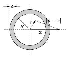
Figure 1: Model scheme used to describe the craniopharyngioma.

II.1 $\beta$ sources

In the case of $\beta$ sources, dosimetry calculations can be performed on the basis of the Loevinger formula Loe56 , which gives the absorbed dose distribution around a point source of a $\beta$-emitting radionuclide in a homogeneous infinite medium. In this approach the absorbed dose rate at a distance $x$ from the point source is given by

$$J_{\beta}(x)\,=\,T_{1}(x)\,+\,T_{2}(x)\,,$$ (2)

where

$$T_{1}(x)\,=\,\left[\frac{Bt}{x^{2}}\,-\,\frac{B}{x}\,\exp\left(1-\frac{x}{t}\right)\right]\,\Theta(t-x)$$ (3)

and

$$T_{2}(x)\,=\,\frac{B}{x}\,\exp\left(1-\frac{x}{z}\right)\,.$$ (4)

In previous equations, $z=(\rho\nu)^{-1}$ and $t=cz$ are characteristic distances, $\rho$ the density of the homogeneous medium, $\nu$ an apparent absorption coefficient and $c$ a dimensionless parameter. The normalization constant $B$ is evaluated by imposing that all the emitted energy is absorbed in a very large sphere, and is given by

$$B\,=\,\displaystyle\frac{1}{4\pi}\,\rho\,\nu^{2}\,\alpha\,\overline{E}_{\beta}\,,$$

with

$$\alpha\,=\,\left[3c^{2}\,-\,(c^{2}-1)\exp(1)\right]^{-1}$$

and $\overline{E}_{\beta}$ the average energy per disintegration. Finally,

$$\Theta(r)\,=\,\left\{\begin{array}[]{ll}0\,,&r<0\,;\\ 1\,,&r>0\,.\end{array}\right.$$

The parameters $\nu$ and $c$ are characteristic of each $\beta$-emitter. For the first one, Loevinger et al. Loe56 gave the following numerical parameterization:

$$\nu\,=\,\displaystyle\frac{18.6}{\left(E_{\beta}^{\rm max}-0.036\right)^{1.37}}\,\left(2-\frac{\overline{E}_{\beta}}{\overline{E}^{*}_{\beta}}\right)\,,$$

where $E_{\beta}^{\rm max}$ is the maximum energy of the electrons emitted by the source, in MeV, and $\nu$ is in cm² g^-1. $\overline{E}^{*}_{\beta}$ is the average energy for a hypothetical $\beta$ disintegration of allowed type with the same maximum energy. The $c$ parameter was parameterized as Loe56 :

$$c\,=\,\left\{\begin{array}[]{ll}2\,,&0.17~{}{\rm MeV}<E_{\beta}^{\rm max}<0.5~{}{\rm MeV}\,;\\ 1.5\,,&0.5~{}{\rm MeV}\leq E_{\beta}^{\rm max}<1.5~{}{\rm MeV}\,;\\ 1\,,&1.5~{}{\rm MeV}\leq E_{\beta}^{\rm max}<3~{}{\rm MeV}\,.\end{array}\right.$$

Adopting this approach for the point absorbed dose rate, the integral in Eq. (1) can be evaluated analytically (see Appendix) and using Eq. (A) we can write

$$\dot{D}_{\beta}(x) = A\,\left\{\displaystyle\frac{\pi Bt}{2x}\left(t\left[12x-11t+4(t-R)\exp\left(\displaystyle\frac{t+R-x}{t}\right)\right]\right.\right.$$

$$\left.~{}~{}~{}~{}~{}~{}+\,3R^{2}+2Rx-5x^{2}+2(R^{2}-x^{2})\ln\left(\displaystyle\frac{t}{x-R}\right)\right)\,\Theta(R+t-x)$$

$$\left.~{}~{}~{}~{}+\displaystyle\frac{2\pi Bz^{2}}{x}\exp\left(\frac{z-R-x}{z}\right)\left[(R+z)+(R-z)\exp\left(\frac{2R}{z}\right)\right]\right\}\,\Theta(x-R)\,.$$

II.2 Photon sources

When $\beta\gamma$-emitters are used, the photon dosimetry is usually based on the formula of Berger Ber68 . In this approach, a photon point isotropic source is assumed to deposit a dose rate at a distance $x$ from the source which is given by

$$J_{\gamma}(x)\,=\,\frac{1}{4\pi}\,\frac{\mu_{\rm en}}{\rho}\,E_{\gamma}\,\frac{1}{x^{2}}\,\exp(-\mu x)\,B_{\rm en}(\mu x)\,.$$ (6)

Here $\mu_{\rm en}$ and $\mu$ are the linear photon energy-absorption and the linear photon attenuation coefficients, respectively, at the energy of the emitted photon, $E_{\gamma}$, and $B_{\rm en}$ is the energy-absorption buildup factor, which takes into account the contribution of the scattered photons. Following Ref. Ber68 , the buildup factors are expanded as

$$B_{\rm en}(\mu x)\,=\,\sum_{n=0}^{10}\,b_{n}\,(\mu x)^{n}\,.$$ (7)

Here $b_{0}=1$ and the remaining coefficients were calculated in Ber68 for some energies ranging from 10 keV to 3 MeV.

As in the case of the Loevinger formula, the integral in Eq. (1) can be calculated analytically for the dose rate in Eq. (6), in the case of the uniform spherical radionuclide distribution we are assuming here (see Appendix). From Eq. (22) we have

$$\dot{D}_{\gamma}(x)\,=\,-A\,\frac{\mu_{\rm en}}{\rho}\,\frac{1}{4x}\,E_{\gamma}\,\sum_{j=0}^{N+3}\,r_{j}(x)\,K_{j}(x)\,,$$ (8)

where the different terms are defined in Eqs. (23)-(28).

II.3 Simulation procedure

MC simulations were performed by using the code PENELOPE Sal01 . PENELOPE is a general purpose MC code which allows to simulate the coupled electron-photon transport. Analog simulation is performed for photons. For electrons, the simulation is carried out in a mixed scheme where collisions are characterized as hard and soft. After fixing a value for a critical angle, the collisions with scattering angles larger than the critical value are called hard collisions and are simulated individually. The collisions with scattering angle smaller than the critical value are called soft collisions and are described by means of a multiple scattering theory. The electron tracking is controlled by four parameters. Two of them, called $C_{1}$ and $C_{2}$, refer to elastic collisions. The first one, $C_{1}$, gives the average angular deflection due to an elastic hard collision and to the soft collisions previous to it. The second parameter, $C_{2}$, represents the maximum value permitted for the average fractional energy loss in a step. The other two parameters, called $W_{\rm cc}$ and $W_{\rm cr}$ are energy cutoffs to distinguish hard and soft events. Thus, the inelastic electron collisions with energy loss $W<W_{\rm cc}$ and the emission of Bremsstrahlung photons with energy $W<W_{\rm cr}$ are considered in the simulation as soft interactions.

For arbitrary materials, PENELOPE can be applied for energies up to 1 GeV and down to few hundred eV, in the case of electrons, and 1 keV, for photons. Besides, PENELOPE permits a good description of the particle transport at the interfaces and presents a more accurate description of the electron transport at low energies in comparison to other general purpose MC codes. These characteristics make PENELOPE to be an useful tool for medical physics applications as previous works have pointed out (see e.g. Refs. San98 -Ase02 ). Details about the physical processes considered can be found in Ref. Sal01 .

In our simulations, the cyst was supposed to be surrounded by an infinitely extended water volume. Both, the spherical layer simulating the craniopharyngioma as well as the colloid introduced into the cyst were assumed to be made of different materials. Thus, we labelled the dose rates obtained with the simulations as $\dot{D}_{\omega}^{\rm vs}$, where the subscript $\omega$ refers to $\beta$ or $\gamma$ according to the primary particle emitted and the superscripts v and s indicate, respectively, the materials of which the inner volume and the spherical shell are made of. Here we considered four materials: soft tissue (t), compact bone (b), gel (g) and water (w). The respective compositions are given in Table 1.

	Composition [atoms/molecule]
	Soft tissue (ICRU)	Compact bone (ICRU)	Gel
Density [g cm-3]	1.0	1.85	1.2914
H	0.10117	0.52790	0.54697
C	0.11100	0.19247	0.23524
N	0.02600	0.01603	0.05393
O	0.76183	0.21311	0.16156
Mg		0.00068
P		0.01879
S		0.00052	0.00230
Ca		0.03050

Table 1: Composition of the different materials used in the MC simulations performed in this paper.

The point sources representing the radionuclide were assumed to be uniformly distributed inside the craniopharyngioma. The direction of the emitted particles was supposed to be isotropic around the initial position. For electrons, the initial energy was sampled from the corresponding Fermi distributions, taken from Ref. Gar85 . For photons, the initial energy was sampled according to the relative intensity of the different energies of the corresponding spectra.

Electrons and photons were simulated for energies above 100 eV and 1 keV, respectively. Below these energies, the particles were considered to be locally absorbed. The simulation parameters were fixed to the values: $W_{\rm cc}=5$ keV, $W_{\rm cr}=1$ keV, $C_{1}=C_{2}=0.05$.

Due to the spherical symmetry of the adopted SVS geometry, the dose distributions were supposed to be functions of the distance to the center of the distribution, $x$. The full simulation volume was subdivided into spherical shells with radial thickness of 0.5 mm. The energy deposited in each voxel was scored to obtain the corresponding histograms.

The statistical uncertainties were calculated by scoring both the energy deposited in a voxel and its square for each history. The average energy deposited in the $k$-th bin (per incident particle) is

$$E_{k}\,=\,\frac{1}{N}\sum_{i=1}^{N}e_{i,k}\,,$$

where $N$ is the number of simulated histories and $e_{i,k}$ is the energy deposited by all the particles of the $i$-th history (that is, including the primary particle and all the secondaries it generates). The statistical uncertainty is given by

$$\sigma_{E_{k}}\,=\,\sqrt{\frac{1}{N}\left[\frac{1}{N}\sum_{i=1}^{N}e_{i,k}^{2}\,-\,E_{k}^{2}\right]}\,.$$

In our calculations, $5\cdot 10^{6}$ histories were simulated in each run.

III Results

III.1 Pure $\beta$ radionuclides

We started by considering a pure $\beta$ emitter as radionuclide in the colloid: the ³²P nucleus. The $\beta$-spectrum of this isotope has a maximum energy $E_{\beta}^{\rm max}=1.71$ MeV with a mean energy $\overline{E}_{\beta}=0.695$ MeV. The decay transition to ³²S is of allowed type and the parameters entering in the Loevinger formula are $c=1$ and $\nu=9.18$ cm² g^-1. Initially we analyzed cysts with $R=1.75$ cm and $\delta=1$ mm, while the activity concentration of the radiocolloid was supposed to be 1 MBq cm^-3.

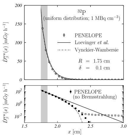
Figure 2: Dose rate in water for a spherical source of ³²P with $R=1.75$ cm, $\delta=0.1$ cm and an activity concentration of 1 MBq cm^-3. The distance of the target point to the center of the distribution is labelled $x$. Dots are for the MC calculation (Error bars correspond to 1$\sigma$ and are smaller than the size of the symbol used). Solid curve gives the result obtained from the Loevinger formula while dashed-dotted curve correspond to the Vynckier-Wambersie formula. The lower panel shows the same results in semilogarithmic scale. Besides the MC results obtained switching it off Bremsstrahlung are plotted with black squares.

First, we have assumed that both the inner volume and the layer were made of water. In this situation (uniform and infinite homogeneous medium), the results of the simulation can be compared directly with our analytical calculations based on the Loevinger approach (Eq. (II.1)) or other analytical approaches such as that of Vynckier and Wambersie Vyn82 . In this last method the $\beta$ point kernels generated were more accurate than those in the Loevinger approach. The results are shown in the upper panel of Fig. 2, where the full and dashed curves show the results obtained with the Loevinger and Vynckier and Wambersie approaches, respectively, and the open squares are the results of our MC simulation. In the lower panel, the same results are plotted in semilogarithmic scale in order to emphasize the differences at large distances. In Table 2 we show the values of the relative differences calculated as:

$$\Delta^{\rm(A,B)}_{\beta}(x)\,=\,\displaystyle\frac{\left[\dot{D}_{\beta}^{\rm ww}(x)\right]_{\rm A}\,-\,\left[\dot{D}_{\beta}^{\rm ww}(x)\right]_{\rm B}}{\left[\dot{D}_{\beta}^{\rm ww}(x)\right]_{\rm B}}\,,$$ (9)

where the subscripts A and B stand for the Loevinger (L) and Vynckier and Wambersie (VW) approaches or the MC simulation. As we can see, Loevinger and MC results agree rather well up to $x\sim 2$ cm. Above this point, the disagreement is apparent, but the value of the dose rate is, at least, one order of magnitude smaller than the dose rate in the cyst wall. Vynckier and Wambersie model provides a slightly better result up to $x\sim 2.3$ cm. At larger distances, the Vynckier and Wambersie approach goes to zero, but there the dose rate is, at least, three orders of magnitude below that in the wall. Similar results are obtained if the $\beta$ point kernels used are those provided by Berger Ber71 .

	$\Delta^{\rm(A,B)}_{\beta}(x)$ [%]
$x$ [cm]	(L,MC)	(VW,MC)	(VW,L)
1.775	-1.1	-2.8	-1.7
1.825	2.6	-2.0	-4.4
1.875	5.5	-2.6	-7.7
1.925	10.0	-3.8	-12.5
1.975	17.2	-5.3	-19.2
2.025	30.7	-5.7	-27.8
2.125	92.4	-5.1	-50.6
2.225	258.3	-17.2	-76.9
2.325	754.5	-68.3	-96.3
2.425	921.5	-100.0	-100.0
2.525	386.8	-100.0	-100.0
3.025	-93.6	-100.0	-100.0
3.525	-99.9	-100.0	-100.0
4.025	-100.0	-100.0	-100.0
4.525	-100.0	-100.0	-100.0
5.025	-100.0	-100.0	-100.0

Table 2: Relative differences (see Eq. (9)) in % between the results obtained for ³²P, in the case of unique medium, with the Loevinger (L) and Vynckier and Wambersie (VW) approaches and MC simulation.

To finish the discussion for a unique medium, we analyzed the role of the Bremsstrahlung radiation. PENELOPE includes this mechanism and, in order to estimate its importance we have performed a new simulation by switching it off. The results obtained are plotted with black squares in the lower panel of Fig. 2. As we can see, the effect of the Bremsstrahlung shows up above $\sim 2.4$ cm. However, at that distance, the dose deposited is four orders of magnitude smaller than the dose delivered to the cyst wall. On the other hand, we can see that the Vynckier and Wambersie model does not include Bremsstrahlung at all, while the Loevinger approach takes it into account in a somehow average way. Despite this, the conclusion is that these analytical approaches permit a reasonable description of the dose rate delivered by this kind of extended sources within a unique medium.

The next step was to investigate the role played by the interfaces present in the craniopharyngioma. The idea was to elucidate, by using MC simulation, if the various interfaces and materials modify the dosimetry provided by the Loevinger approach. To measure the effect of the presence of the different materials, we calculated the relative differences

$$\Delta^{\rm v^{\prime}s^{\prime}-vs}_{\omega}({\rm cyst})\,=\,\displaystyle\frac{\dot{D}_{\omega}^{\rm v^{\prime}s^{\prime}}({\rm cyst})\,-\,\dot{D}_{\omega}^{\rm vs}({\rm cyst})}{\dot{D}_{\omega}^{\rm vs}({\rm cyst})}\,,$$ (10)

where

$$\dot{D}_{\omega}^{\rm vs}({\rm cyst})\,=\,\displaystyle\frac{1}{\rho_{\rm s}v_{\rm s}}\sum_{k}E_{k}$$ (11)

are the integral dose rates delivered inside the cyst wall. Here $k$ runs over all the bins contained inside the cyst wall, $\rho_{\rm s}$ is the density of the material forming this wall and $v_{\rm s}$ is its volume.

		$\Delta^{\rm v^{\prime}s^{\prime}-vs}_{\beta}({\rm cyst})$ [%]
$R$ [cm]	$\delta$ [mm]	wt-ww	wb-ww	gt-wt	gb-wb	gt-ww	gb-ww
1.75	1.0	0.87	-28.02	-20.67	-20.61	-19.99	-42.86
1.75	2.0	1.18	-39.65	-21.15	-21.24	-20.22	-52.47
1.75	3.0	0.98	-44.77	-20.81	-20.99	-20.03	-56.37
1.00	1.0	0.46	-27.39	-20.62	-20.58	-20.25	-42.34
2.50	1.0	0.50	-28.44	-20.50	-21.02	-20.11	-43.48

Table 3: Relative differences in %, as given by Eq. (10), for ³²P in the different cases analyzed in this paper (see text).

We have first studied the effect of the material forming the spherical shell which represents the craniopharyngioma. We have considered two extreme cases: soft tissue and compact bone. The differences of the dose rates calculated with MC in both situations with respect to $\dot{D}_{\beta}^{\rm ww}(x)$ are shown in panels (a) and (b) of Fig. 3. The relative differences in the cyst wall are given in Table 3. As we can see, the presence of the soft tissue in the spherical shell leaves practically unmodified the dosimetry. In fact, the total dose rate delivered to this shell increases by only 0.9% in this case. On the contrary, when the bone is considered the dose received by the wall reduces 28.0%. Furthermore, the dose rate delivered to the external medium nearby the craniopharyngioma diminishes appreciably in the case of the bone, while no modifications are observed for soft tissue. Obviously, these modifications are not considered in the analytical expressions based on the Loevinger approach.

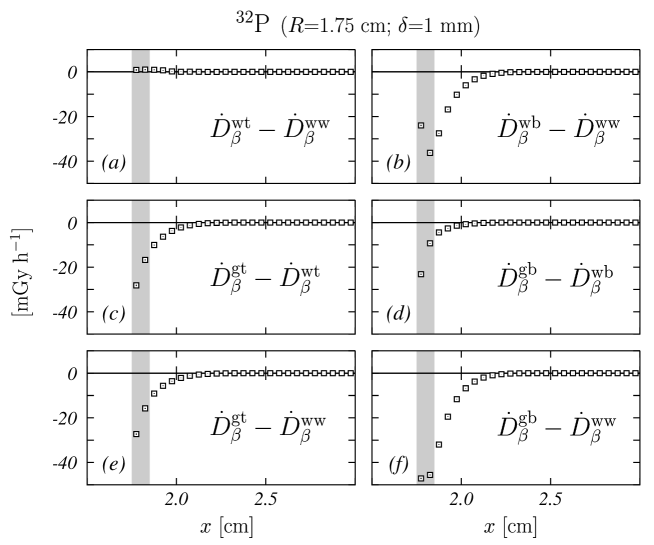
Figure 3: Effect of the materials considered for the spherical shell which represents the cystic wall in our model and for the inner volume. Panels (a) and (b) show the effect of considering the wall of the craniopharyngioma to be done of soft tissue and bone, respectively. Panels (c) and (d) show the effect due to the substitution of the water by the gel in the inner volume. Finally, panels (e) and (f) show the full effect due to the presence of these materials with respect to the reference dose rate $\dot{D}_{\beta}^{\rm ww}(x)$. The shadow region shows the cystic wall which has been considered to have a thickness $\delta=1$ mm. Error bars correspond to 1$\sigma$ and are smaller than the size of the symbol used.

In the treatment procedure, the radionuclide is introduced in the craniopharyngioma inner volume, embedded in a certain type of colloid. In our simulations we have considered the gel with the composition given in Table 1. In panels (c) and (d) of Fig. 3 we show the differences in the dose rates obtained when the water is substituted by the gel in the inner volume. As we can see, the gel produces a noticeable reduction of the dose delivered to the cyst wall. This reduction reaches 20.7% in the case of soft tissue and 20.6% in the case of the bone. Besides, also the dose delivered to the surrounding outer volume reduces.

The net effect due to the presence of both gel in the inner volume and soft tissue or bone in the craniopharyngioma, in relation to the case in which only water is considered, is shown in panels (e) and (f) of Fig. 3. The dose rate delivered to the cyst wall reduces in 20.0%, in the case of the soft tissue, and 42.9% in the case of bone. Even if we can expect that the craniopharyngioma is composed of a material with an intermediate density, the dose rate delivered to both, the cyst wall and the outer volume nearby it, would be strongly reduced in relation to what it is obtained using the Loevinger approach.

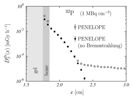
Figure 4: Effect of the Bremsstrahlung radiation for the case in which gel and bone are present in the inner volume and the wall of the craniopharyngioma, respectively. Black squares give the dose rate obtained when Bremsstrahlung mechanism is switched off. Open squares correspond to the full calculation.

The presence of materials with densities larger than that of water, could make the Bremsstrahlung effect more important. As before, we have carried out a new simulation (for the case in which gel and bone are present in the inner volume and in the wall of the craniopharyngioma, respectively), but we switched off the Bremsstrahlung mechanism. In Fig. 4 the results obtained (black squares) are compared to those of the full calculation (open squares). These results are rather similar to those found for the case of a unique medium (see lower panel in Fig. 2), except for two details. First, the Bremsstrahlung effect begins to be observed in the radiation queue at a slightly shorter distance, $\sim 2.2$ cm. Second, the inclusion of Bremsstrahlung effects produces an increase of the dose delivered to the cyst wall which reaches the non negligible value of $\sim 45$%. If we compare the simulation without Bremsstrahlung with the analytical approaches which, as mentioned previously, do not treat this effect in an adequate way, the reduction observed for the dose delivered to the cyst wall would be even larger.

At this point, it is necessary to clarify how the previous conclusions are related to the choice of the geometry. For this reason we have performed a set of calculations similar to the previous ones but assuming different thicknesses for the tumor wall and different sizes for the inner volume.

First we have analyzed the effect of the wall thickness and we have considered $\delta=2$ and 3 mm. The relative differences $\Delta^{\rm v^{\prime}s^{\prime}-vs}_{\beta}({\rm cyst})$ obtained are shown in Table 3 for different materials and configurations. As we can see, the effect of the presence of the soft tissue is rather small, increasing the dose delivered to the cyst by $\sim 1$% (see third column). On the contrary, the fact that the wall is made of bone produces a considerable reduction of the dose rate in it. Besides, this reduction grows with the thickness of the cyst wall (see fourth column).

The effect of the presence of the gel in the inner volume seems to be almost independent of the thickness of the wall producing a reduction of $\sim 20$% in all cases (see fifth and sixth columns).

Finally, the combined effect of soft tissue in the wall and of the gel in the inner volume (seventh column) is practically equal to that of the gel alone, while in the case of bone (eight column), the reduction increases with the wall thickness, following the behavior observed when no gel was considered. It is worth to point out that the dose rate delivered to the cyst can be diminished by more than 50%.

To study the influence of the inner volume of the craniopharyngioma we have considered two different values of its radius: $R=1$ and 2.5 cm. In both calculations we have maintained the activity concentration of 1 MBq cm^-3. The results obtained in the simulations are shown in the two last rows of Table 3. As we can see, the values of the relative differences are very similar to those found for the former calculation ($R=1.75$ cm, $\delta=1$ mm). This indicates that the important parameter is the thickness of the cyst wall. The reduction of the dose delivered to it becomes bigger with the increase of the thickness.

III.2 $\beta\gamma$ sources

After having analyzed the case of pure $\beta$ sources, we studied $\beta\gamma$ sources. To perform the calculations we have considered the ¹⁸⁶Re radionuclide which has the decay scheme shown in Fig. 5 Chu99 . Following Ref. Ann98 , in order to simplify the simulation, we considered only the most relevant transitions, whose properties are given in Table 4. In this table, we show for X-rays, internal conversion (IC) and Auger electrons (these last two have been grouped) the average values of the energies and the intensities. The two $\beta$ decays considered are first forbidden (not unique). However, the sampling procedure Gar85 is the same as for allowed transitions.

Figure 5: Decay scheme of the ¹⁸⁶Re radionuclide. In actual simulations, only the $\beta$ decays populating the ground and the first excited state of the ¹⁸⁶Os, the $\gamma$ decays shown with solid lines as well as the X-rays and IC and Auger electrons mentioned in the text have been considered.

Type	Energy [keV]	Absolute intensity [%]
$\beta^{-}$	1069.50	70.99
$\beta^{-}$	932.34	21.54
$\gamma$	767.50	0.03
$\gamma$	630.34	0.03
$\gamma$	137.16	9.42
$\gamma$	122.30	0.60
W K X-rays	$\sim$65.00	6.00
Os K X-rays	$\sim$65.00	3.50
IC+Auger	$\sim$14.00	22.00

Table 4: Characteristic radiations considered in this paper for the decay of the ¹⁸⁶Re. The energies given for the $\beta^{-}$ are the endpoint energies. Data have been obtained from Refs. Chu99 ; Ann98 .

As in the previous case, we assumed a source of $R=1.75$ cm with $\delta=1$ mm and an activity concentration of 1 MBq cm^-3 introduced in the inner volume of the craniopharyngioma.

We began by comparing to the theoretical predictions based on the Loevinger and Berger approaches, our MC simulations, done by assuming a unique medium (water).

For the $\beta$ decay with $E_{\beta}^{\rm max}=1.069$ MeV, the mean energy is $\overline{E}_{\beta}=0.362$ MeV and the parameters entering in the Loevinger formula are $c=1.5$ and $\nu=17.78$ cm² g^-1. For that with $E_{\beta}^{\rm max}=0.932$ MeV, we used $\overline{E}_{\beta}=0.309$ MeV, $c=1.5$ and $\nu=21.61$ cm² g^-1. The results corresponding to $\dot{D}_{\beta}^{\rm ww}(x)$ are shown in Fig. 6. The calculations have been done by using the absolute intensities given in Table 4. As we can see, the simulation (dots) and the analytical calculation (solid lines) show a good agreement, as it happened in the case of ³²P.

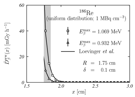
Figure 6: Same as Fig. 2 but for the two main $\beta$ decays of ¹⁸⁶Re. Only the Loevinger approach results are shown. The absolute intensities of both emissions are included.

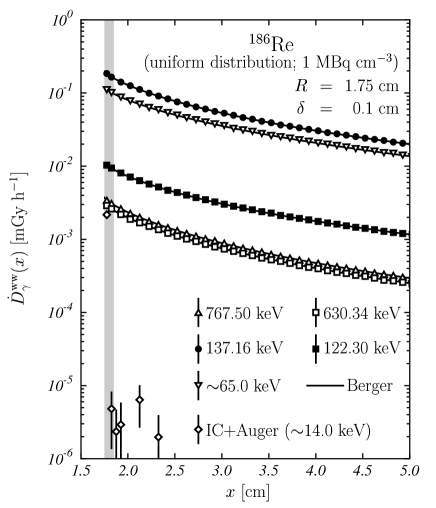
Figure 7: Same as Fig. 2 but for the main $\gamma$ and X-ray radiations of ¹⁸⁶Re. Solid curves show the result obtained from the Berger approach. The absolute intensities of the different emissions are included.

The results obtained for the remaining radiations in Table 4 are shown in Fig. 7. Also in these results, the absolute intensities of each radiation are included. For photons (these are the four $\gamma$ emissions and the X-rays), the results of the simulations (dots) are compared with those provided by the analytical approach of Berger (solid lines). The parameters entering in Eq. (22), and given in Table 5, have been obtained by performing cubic interpolations of the values quoted in Ref. Ber68 . It is remarkable the excellent agreement between the analytical approach and the MC simulation. It is also worth to notice that the $\gamma$ emissions with $E_{\gamma}=137.16$ keV and the X-ray of W and Os are the most important contributions here, while the other emissions are more than one order of magnitude smaller.

$E_{\gamma}$ [keV]	65	122.30	137.16	630.34	767.50
$\mu$ [cm]	0.191	0.158	0.153	0.087	0.080
$\mu_{\rm en}$ [cm]	0.0292	0.02613	0.02691	0.0328	0.0322
$b_{1}$	2.50964594E+00	1.77904308E+00	1.6780888E+00	9.16518331E-01	8.59057903E-01
$b_{2}$	1.42232013E+00	1.10754991E+00	9.9470758E-01	3.82239223E-01	3.56937379E-01
$b_{3}$	1.86807606E-02	1.91051394E-01	1.8541029E-01	4.75710258E-02	-1.91028565E-02
$b_{4}$	1.71705126E-03	-5.35412366E-03	-6.1609102E-03	-4.75984300E-03	-4.22946505E-05
$b_{5}$	-9.58392775E-06	6.26657449E-04	7.3442928E-04	9.06498346E-04	3.30697017E-04
$b_{6}$	3.01566342E-06	-1.99327806E-05	-3.3124285E-05	-8.57197738E-05	-4.32139241E-05
$b_{7}$	-2.95050882E-07	1.93571609E-07	1.0333482E-06	4.61301079E-06	2.68527947E-06
$b_{8}$	1.26480826E-08	1.07387210E-08	-1.9661881E-08	-1.42838076E-07	-9.03993893E-08
$b_{9}$	-2.53243121E-10	-3.77658183E-10	1.9686815E-10	2.36108977E-09	1.57900648E-09
$b_{10}$	1.96279971E-12	3.65828331E-12	-7.2484147E-13	-1.60724663E-11	-1.11767913E-11

Table 5: Parameters to be used in the analytical approach based on the Berger formula discussed in this paper. The medium considered is water. The different radiations correspond to the $\gamma$ and X-ray emissions taken into account for ¹⁸⁶Re. The value of the parameter $b_{0}$ is fixed to 1 for all energies.

		$\Delta^{\rm v^{\prime}s^{\prime}-vs}_{\beta,\gamma}({\rm cyst})$ [%]
Type	Energy [keV]	gw-ww	gb-ww
$\beta^{-}$	1069.50	-20.37	-52.21
$\beta^{-}$	932.34	-20.90	-54.34
$\gamma$	767.50	-0.33	-3.26
$\gamma$	630.34	-1.86	-4.30
$\gamma$	137.16	-0.97	31.55
$\gamma$	122.30	-1.51	47.30
X-rays	$\sim 65.0$	-0.24	217.38
IC+Auger	$\sim 14.0$	-20.25	-57.89
Full spectrum		-20.26	-51.19

Table 6: Relative differences in %, as given by Eq. (10), for the different radiations of ¹⁸⁶Re. Here $R=1.75$ cm and $\delta=1$ mm. Last row gives the results for the full spectrum of ¹⁸⁶Re considered in this paper. The energies given for the $\beta^{-}$ are the endpoint energies.

In Fig. 7 we also show the results the IC and Auger electrons (diamonds). These phenomena cannot be described by the analytical approaches considered here but, in any case, their contribution seems to be negligible.

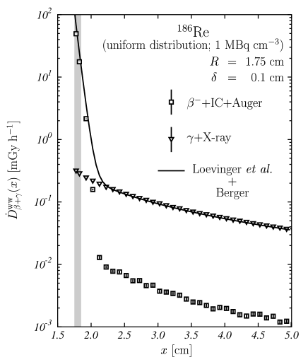
Figure 8: Same as Fig. 2 but for the full spectrum emission of ¹⁸⁶Re. The separate contribution of the $\beta$ emission plus IC and Auger electrons (squares) and that of $\gamma$ plus X-rays (triangles) are shown. Solid curve shows the analytical result obtained from the Loevinger and Berger approaches.

In Fig. 8 we show the separate contributions of the electrons, say $\beta$ emissions, IC and Auger electrons (squares), and of the photons, $\gamma$ emissions and X-rays (triangles). The solid curve corresponds to the analytical calculation performed by summing the contributions obtained with the Loevinger approach for the two $\beta$ emissions and with the Berger approach for the $\gamma$ emissions and the X-rays. As we can see it provides a rather good description of the simulated results. Besides, it is worth to point out that the dose delivered to the craniopharyngioma is mainly due to the $\beta$ radiation, the photon contribution being two orders of magnitude smaller. On the contrary, the dose due to electrons becomes more than one order of magnitude smaller than the one delivered by $\gamma$ emissions and X-rays for $x>2$ cm, that is at distances above 2 mm far from the outside surface of the craniopharyngioma.

Finally, we have tested the effect of the different materials and interfaces in the dosimetry. First, we have evaluated the dose rate by assuming gel in the inner volume of the craniopharyngioma. The results corresponding to the relative differences, as given by Eq. (10), are those in the third column of Table 6. In this table we also show the values for each of the radiations considered in the spectrum of the ¹⁸⁶Re and, in the last row, for the full spectrum (by including the proper absolute intensities). As we can see, the presence of the gel produces a reduction of the dose delivered to the cyst wall. This reduction is of $\sim 20$% for the $\beta$ emissions and for the IC and Auger electrons. The reduction, no greater than 2%, is very small for $\gamma$ and X-ray radiations. The full effect of the gel is 20.3% reduction, as expected due to the dominance of the $\beta$ radiations previously discussed.

In a second step we have studied the effect of the material forming the cyst wall. We have checked that, as it happened for the ³²P radionuclide, the presence of soft tissue, instead of water, produces negligible modifications. In the last column of Table 6 we show the results obtained when compact bone is assumed to constitute the cyst wall. As we can see, the reduction of the dose delivered to the cyst reaches more than 50% for the $\beta$, IC and Auger electron emissions. However, the behavior for $\gamma$ radiations is different. While for the more energetic photons the dose reduces (less than 5%), it increases considerably for the less energetic ones, with an enormous enhancement (more than 200%) for X-rays. In any case, the dominance of the $\beta$ emissions on the full spectrum is again remarkable.

The average energies of the $\beta$ emissions in this radionuclide are smaller than these of ³²P. This implies that Bremsstrahlung effect is less important in this case. On the other hand, we have check that the Bremsstrahlung effect for the $\gamma$ emissions is negligible, the dose rates obtained without Bremsstrahlung overlapping with those found in the full calculation.

To finish, we compare the integral dose rates (see Eq. (11)) delivered by the two radionuclides here considered inside the cyst wall. In the case of a unique medium (water) and assuming the same radionuclide concentration injected in the inner volume of the cyst, the dose rate deposited in the wall by the ¹⁹⁸Re is 33% smaller than the one due to ³²P. When we consider the cyst filled with gel and the cyst shell made of bone, the dose rate of ¹⁹⁸Re is 25% smaller than that of ³²P.

IV Conclusions

In this paper we have investigated the dosimetry for radiocolloid therapy of cystic craniopharyngiomas. The craniopharyngioma has been described as a spherical shell with given internal radius and thickness. Different materials have been considered to form the colloid introduced in the craniopharyngioma and the shell representing the cyst wall. Explicit analytical expressions for the dose rate due to $\beta$ and $\gamma$ emitters have been obtained on the base of the well known Loevinger and Berger formulae for point sources. Results for ³²P and ¹⁸⁶Re are quoted.

The results obtained with these analytical expressions, valid under the assumption of a unique medium, have been compared with calculations performed with the Monte Carlo simulation code PENELOPE. These calculations show a nice agreement for both $\beta$ and $\gamma$ emissions in the two radionuclides studied.

By using the Monte Carlo simulation, the role of the different materials and of the interfaces present in the problem, has been investigated. The main conclusions we draw are the following ones.

1. The effect of the material forming the colloid (gel in our case) produces a reduction of $\sim 20$% of the dose delivered to the cyst wall by $\beta$ and IC and Auger electron emissions. This reduction is smaller than 2% for $\gamma$ and X-ray emissions.

2. There are no noticeable differences between the results obtained when soft tissue or water are considered to form the cyst wall.

3. The consideration of compact bone as the material forming the cyst wall gives rise to relevant effects. For $\beta$ and IC and Auger electron emissions, the dose delivered to the cyst wall reduces by a factor larger than 25%. This effect together with that produced by the colloid makes this dose to be reduced by more than 40%. For $\gamma$ and X-ray emissions, the presence of the bone in the cyst wall appears to be very important for energies below 200 keV. In this situation, the dose delivered to the cyst wall increases by more than 200% in the case of the X-rays of 65 keV we have considered. For the ¹⁸⁶Re the dominant emissions are $\beta$ radiations, and they obscure this enormous effect.

4. All the effects quoted above, do not change with the size (inner radius) of the craniopharyngioma, but increase with its thickness, which appear to be the relevant parameter to consider in the dosimetry.

Appendix A Formulae for spherical uniform sources

In this appendix we discuss the procedure to calculate analytically the integral in Eq. (1) for the point dose rates corresponding to the Loevinger and Berger approaches.

In the first case, and taking into account Eq. (2), the dose rate per activity unit at a distance $x$ from the center of the distribution can be written as

$$\frac{1}{A}\,\dot{D}_{\beta}(x)\,=\,I_{1}(x)\,+\,I_{2}(x)\,,$$ (12)

where

$$I_{i}(x)\,=\,\int_{\rm V}\,{\rm d}\textbf{r}\,T_{i}(\left|\textbf{x}-\textbf{r}\right|)\,.$$ (13)

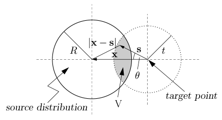
Figure 9: Geometrical scheme to calculate the integrals of the Loevinger and Berger formulae for an extended spherical source uniformly distributed.

The key point to evaluate the corresponding integrals is to fix the center of the coordinate system on the target point. The scheme is represented in Fig. 9. In the case of the integral $I_{1}(x)$, one has to consider that $T_{1}(x)$ has a range $t$ (see Eq. (3)). Thus, the only contribution to the integral comes from points inside the source distribution and sited at a distance $s\leq t$ from the target point. Therefore, only the shadowed volume shown in Fig. 9 contributes to $I_{1}(x)$ and we have

$$I_{1}(x) = \int_{\rm V}\,{\rm d}\textbf{s}\,T_{1}(s)\,=\,\int_{x-R}^{t}\,{\rm d}s\,s^{2}\,T_{1}(s)\,\int_{0}^{\theta_{\rm max}}\,{\rm d}\theta\sin\theta\,\int_{0}^{2\pi}\,d\phi$$ (14)

$$= 2\pi\,\int_{x-R}^{t}\,{\rm d}s\,s^{2}\,T_{1}(s)\,\int_{0}^{\cos\theta_{\rm max}}\,{\rm d}(-\cos\theta)$$

$$= 2\pi\,\int_{x-R}^{t}\,{\rm d}s\,s^{2}\,\left(1-\cos\theta_{\rm max}\right)\,T_{1}(s)\,.$$

The angle $\theta_{\rm max}$ is the value reached by $\theta$ when $|\textbf{x}-\textbf{s}|=R$ and then

$$\cos\theta_{\rm max}\,=\,\displaystyle\frac{x^{2}+s^{2}-R^{2}}{2xs}\,.$$ (15)

Considering the above equations, the integral (14) becomes

$$I_{1}(x)\,=\,\displaystyle-\frac{\pi}{x}\,\Theta(x-R)\,\Theta(R+t-x)\,\int_{x-R}^{t}{\rm d}s\,s\,\left[(x-s)^{2}-R^{2}\right]\,T_{1}(s)\,.$$ (16)

Here, the $\Theta(x-R)$ factor indicates that the calculation is valid for points outside the distribution, while the $\Theta(R+t-x)$ factor points out the fact that this contribution cancels for $x$ values larger than $R+t$. The result of the integration is

$$I_{1}(x) = \displaystyle\frac{\pi Bt}{2x}\left\{t\,\left[12x-11t+4(t-R)\exp\left(\displaystyle\frac{t+R-x}{t}\right)\right]\,+\,3R^{2}+2Rx-5x^{2}\right.$$ (17)

$$\left.~{}~{}~{}~{}~{}~{}~{}~{}+2(R^{2}-x^{2})\ln\left(\displaystyle\frac{t}{x-R}\right)\right\}\,\Theta(x-R)\,\Theta(R+t-x)\,.$$

Note that, in the limit $x=R$ this contribution is

$$I_{1}(R)\,=\,\displaystyle\frac{\pi Bt^{2}}{2R}\left\{4R\left[3-\exp(1)\right]-t\left[11-4\exp(1)\right]\right\}\,.$$ (18)

To calculate the contribution $I_{2}(x)$, a similar procedure is followed. Now, the full source distribution contributes and this implies that in Eq. (16) we must change the upper limit in the integral to $x+R$. Thus one has

$$I_{2}(x) = \displaystyle-\frac{\pi}{x}\,\int_{x-R}^{x+R}{\rm d}s\,s\,\left[(x-s)^{2}-R^{2}\right]\,T_{2}(s)$$ (19)

$$= \displaystyle\frac{2\pi Bz^{2}}{x}\exp\left(\frac{z-R-x}{z}\right)\left[(R+z)+(R-z)\exp\left(\frac{2R}{z}\right)\right]\,.$$

By substituting Eqs. (17) and (19) into Eq. (12) we have finally

$$\frac{1}{A}\,\dot{D}_{\beta}(x) = \left\{\displaystyle\frac{\pi Bt}{2x}\left(t\left[12x-11t+4(t-R)\exp\left(\displaystyle\frac{t+R-x}{t}\right)\right]\right.\right.$$

$$\left.~{}~{}~{}~{}~{}~{}~{}~{}~{}~{}+\,3R^{2}+2Rx-5x^{2}+2(R^{2}-x^{2})\ln\left(\displaystyle\frac{t}{x-R}\right)\right)\,\Theta(R+t-x)$$

$$\left.+\displaystyle\frac{2\pi Bz^{2}}{x}\exp\left(\frac{z-R-x}{z}\right)\left[(R+z)+(R-z)\exp\left(\frac{2R}{z}\right)\right]\right\}\,\Theta(x-R)\,.$$

For $\gamma$ emitters, the integral in Eq. (1) is evaluated for the point dose rate given by the Berger approach (6). In this case, $J_{\gamma}(x)$ has no range and the calculation follows the same steps as those for the $T_{2}$ term of the Loevinger formula. Thus one can write

$$\frac{1}{A}\,\dot{D}_{\gamma}(x)\,=\,\int_{\rm V}\,{\rm d}\textbf{r}\,J_{\gamma}(\left|\textbf{x}-\textbf{r}\right|)\,=\,\displaystyle-\frac{\pi}{x}\,\int_{x-R}^{x+R}{\rm d}s\,s\,\left[(x-s)^{2}-R^{2}\right]\,J_{\gamma}(s).$$ (21)

Substituting Eqs. (6) and (7) here one has

$$\frac{1}{A}\,\dot{D}_{\gamma}(x)\,=\,-\frac{\mu_{\rm en}}{\rho}\,\frac{1}{4x}\,E_{\gamma}\,\sum_{j=0}^{N+3}\,r_{j}(x)\,K_{j}(x)\,,$$ (22)

where

$$r_{j}(x)\,=\,\sum_{i={\rm max}(0,j-N-1)}^{{\rm min}(j,2)}\,a_{i}(x)\,b_{j-i}\,\mu^{j-i}\,,$$ (23)

with

$$a_{i}(x)\,=\,\left\{\begin{array}[]{ll}x^{2}\,-\,R^{2}\,,&i=0\,,\\ -2x\,,&i=1\,,\\ 1\,,&i=2\,,\end{array}\right.$$ (24)

and

$$K_{j}(x)\,=\,\int_{x-R}^{x+R}\,{\rm d}s\,s^{j-1}\,\exp(-\mu s)\,,$$ (25)

If $j=0$ the integral $K_{0}(x)$ is given by Abr72

$$K_{0}(x) = E_{1}\left(\mu(x-R)\right)\,-\,E_{1}\left(\mu(x+R)\right)$$

$$= \ln\displaystyle\frac{x+R}{x-R}\,+\,\sum_{n=1}^{\infty}\,\frac{(-1)^{n}\,\mu^{n}}{n\,n!}\,\left[(x+R)^{n}\,-\,(x-R)^{n}\right]\,,$$

where $E_{1}(x)$ is the exponential integral Abr72 . For $j\not=0$ we have Abr72

$$K_{j}(x)\,=\,\displaystyle\frac{1}{\mu^{j}}\,\left[\gamma\left(j,\mu(x+R)\right)\,-\,\gamma\left(j,\mu(x-R)\right)\right]\,,\,\,\,j\not=0\,,$$ (27)

with

$$\gamma(n,z)\,=\,(n-1)!\,P(n,z)\,=\,(n-1)!\,\left\{1\,-\,\exp(-z)\,\sum_{k=0}^{n-1}\,\frac{z^{k}}{k!}\,.\right\}$$ (28)

- (1) L.J. Rubinstein, Tumors on the central nervous system (Armed Forces Institute of Pathology, Washington DC, 1972).
- (2) K. Shapiro, K. Till and N. Grant, “Craniopharyngiomas in childhood,” J. Neurosurg. 50, 617-623 (1979).
- (3) L. Leksell and L.A. Liden, “A therapeutic trial with radioactive isotopes in cystic brain tumor,” in Radioisotope Techniques. Vol. 1: Medical and Physiological Applications (Her Majesty’s Stationery Office, London, 1953) p. 76.
- (4) H.T. Wycis, R. Robbins, M. Spiegel-Adolph, J. Meszaros and E.A. Spiegel, “Treatment of a cystic craniopharyngioma by injection of radioactive P-32,” Confin. Neurol. 14, 193-202 (1954).
- (5) R. Loevinger, E.M. Japha and G.L. Brownell, “Discrete radioisotope sources,” in Radiation Dosimetry, edited by G.J. Hine and G.L. Brownell (Academic Press, New York, 1956) pp. 694-799.
- (6) J.C. Harbert, J.S. Robertson and K.D. Held, Nuclear medicine therapy (Thieme Medical Publishers, New York, 1987).
- (7) M.J. Berger, “Distribution of absorbed dose around point sources of electrons and beta particles in water and other media,” MIRD Pamphlet No. 7, J. Nucl. Med. Suppl. 5, 7-23 (1971).
- (8) E.L. McGuire, S. Balachandran and C.M. Boyd, “Radiation dosimetry considerations in the treatment of cystic suprasellar neoplasms,” Br. J. Radiol. 59, 779-785 (1986).
- (9) M.J. Berger, “Energy deposition in water by photons from point isotropic sources,” MIRD Pamphlet No. 2, J. Nucl. Med. Suppl. 1, 17-25 (1968).
- (10) M. Abramowitz and I.A. Stegun, Handbook of mathematical functions (Dover Publ. Inc., New York, 1972).
- (11) F. Salvat, J.M. Fernández-Varea, E. Acosta and J. Sempau, PENELOPE, a code system for Monte Carlo simulation of electron and photon transport (NEA-OECD, Paris, 2001).
- (12) A. Sánchez-Reyes, J.J. Tello, B. Guix and F. Salvat, “Monte Carlo calculation of the dose distributions of two 106Ru eye applicators,” Radiother. Oncol. 49, 191-196 (1998).
- (13) J. Sempau, A. Sánchez-Reyes, F. Salvat, H. Oulad ben Tahar, S.B. Jiang and J.M. Fernández-Varea, “Monte Carlo simulation of electron beams from an accelerator head using PENELOPE,” Phys. Med. Biol. 46, 1163-1186 (2001).
- (14) J. Asenjo, J.M. Fernández-Varea and A. Sánchez-Reyes, “Characterization of a high-dose-rate 90Sr-90Y source for intravascular brachytherapy by using the Monte Carlo code PENELOPE,” Phys. Med. Biol. 47, 697-711 (2002).
- (15) International Commision on Radiation Units and Measurements, ICRU Report No. 46, Photon, electron, proton and neutron interaction data for body tissues (ICRU, Bethesda, 1992).
- (16) E. García-Toraño and A. Grau Malonda, “EFFY, a new program to compute the counting efficiency of beta particles in liquid scintillators,” Comput. Phys. Commun. 36, 307-312 (1985).
- (17) S. Vynckier and A. Wambersie, “Dosimetry of beta sources in radiotherapy I. The beta point source dose function,” Phys. Med. Biol. 27, 1339-1347 (1982).
- (18) S.Y.F. Chu, L.P. Ekstr m and R.B. Firestone, “WWW Table of Radioactive Isotopes, database version 2/28/99,” from URL http://nucleardata.nuclear.lu.se/nucleardata/toi/
- (19) M.F. L’Annunziata (ed.), Handbook of radioactivity analysis (Academic Press, San Diego, 1998).