Event Selection Using an Extended Fisher Discriminant Method

Abstract

This note discusses the problem of choosing between hypotheses in a situation with many, correlated non-normal variables. A new method is introduced to shrink the many variables into a smaller subset of variables with zero mean, unit variance, and zero correlation coefficient between variables. These new variables are well suited to use in a neural net.

I Introduction

At the Durham Statistics in Physics Conference (2002), S. Towers1 noted some of the problems that occur when one uses many, correlated variables in a multivariate analysis and proposed a heuristic method to shrink the number. In this note a semi-automatic method is suggested help with this problem. The MiniBooNE experiment is faced with just such a problem, distinguishing $\nu_{e}$ events from background events given a large number of variables obtained from the event reconstructions.

II Fisher Discriminant Method and its Extension

The Fisher discriminant method is a standard method for obtaining a single variable to distinguish hypotheses starting from a large number of variables. If the initial variables come from a multi-normal distribution, the Fisher variable encapsulates all of the discrimination information. However, in many problems the variables are not of this form and the Fisher variable, although useful, is not sufficient.

The Fisher discriminant method 2 finds the linear combination $y$ of the initial variables $x$ which maximizes

$$(\overline{y}_{\rm sig}-\overline{y}_{\rm bkg})^{2}/[{\rm var_{sig}+var_{bkg}}],$$

where $\overline{y}$ is the mean value of the variable and var is the variance. If $S$ is the correlation matrix for the original variables corresponding to the denominator, then the inverse of $S$ dotted into $(\overline{x}_{\rm sig}-\overline{x}_{\rm bkg})$, gives the combination which maximizes the preceding expression.

If the distribution is not multi-normal, there is information still to be obtained after finding the Fisher variable. It is then useful to apply this method successively, firstly to the original variables and, afterwards, to several non-linear transformations of the variables. Presently, three transformations are chosen: the logarithms of the original variables, the exponentials of the original variables and the cube of the original variables. Together with the original variables, this is then four choices. The present note describes a work in progress. It is highly likely that these are not optimum and that better choices can and will be found. Indeed, it is likely that the optimum choice depends on the problem.

The method is also used with the original denominator, $[{\rm var_{sig}+var_{bkg}}]$ and then with each individual variance in turn. This is done since some of the variables may be quite narrow for signal and wide for background or vice versa. (See Figure 1) There are then $4\times 3=12$ variables obtained with this method.

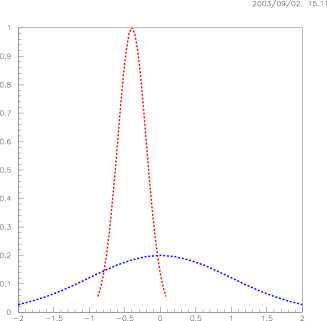
Figure 1: Figure 1: Different Width Normal Distributions

The procedure follows the following steps:

• 1. Start with equal Monte Carlo samples of signal and background events

• 2. Multiply and translate each variable to have an overall mean of zero and unit variance. It is useful to fold variables if necessary to maximize the difference in means. A few events, very far out on the tails of the distribution are clipped ($x>6\sigma$).

• 3. Order the variables according to $|\overline{x}_{\rm sig}-\overline{x}_{\rm bkg}|$ divided by the smallest of the signal and background variances. At present, the ordering of variables is done only once.

• 4. Apply this extended Fisher method to the appropriate transformation of the variables.

• 5. Use the Gram-Schmidt procedure to make the other variables have zero correlation coefficient with the chosen linear combination.

• 6. The new variable is a linear combination of the original $n$ variables. One variable must be discrded to have an independent set. Discard the least significant (by the criterion of step 3) of the original variables. Using the $n-1$ non-Fisher variables, go back to step 2 to get the next variable.

For MiniBooNE the roefitter reconstruction started with 49 particle identification variables. Using the steps outlined, these were reduced to 12 variables. When $\nu_{e}$ quasi-elastic events were compared with background neutral current $\pi^{0}$ events, the use of this procedure with a neural net kept 46% of the $\nu_{e}$ and reduced the $\pi^{0}/\nu_{e}$ ratio to 1.1% of its original value. The neural net was not hard to tune. The reconstruction–particle identification package is still being improved, so these numbers will improve further. The results obtained here are similar to those obtained using a more elaborate neural net on a subsample of 26 of the original 49 variables.

These 12 variables have zero correlation coefficients. Use of the neural net is simplified and it is convenient to look at the effect of cuts using these variables.

Plots of the first nine of the twelve variables are shown in Figure 2.

Figure 2: Figure 2: Plots of the first nine of the variables obtained. The solid lines are the $\nu_{e}$ signal and the dashed lines are the $\pi^{0}$ background.

References

- (1) S. Tower, Benefits of Minimizing the Number of Discriminators Used in a Multivariate Analysis, Durham Conference on Statistics (2002).
- (2) Glen Cowan Statistical Data Analysis, Clarendon Press, Oxford (1998).