Quantum mechanical cumulant dynamics near stable periodic orbits in phase space: Application to the classical-like dynamics of quantum accelerator modes

Abstract

We formulate a general method for the study of semiclassical-like dynamics in stable regions of a mixed phase-space, in order to theoretically study the dynamics of quantum accelerator modes. In the simplest case, this involves determining solutions, which are stable when constrained to remain pure-state Gaussian wavepackets, and then propagating them using a cumulant-based formalism. Using this methodology, we study the relative longevity, under different parameter regimes, of quantum accelerator modes. Within this attractively simple formalism, we are able to obtain good qualitative agreement with exact wavefunction dynamics.

I Introduction

Since their initial discovery Oberthaler1999 , quantum accelerator modes Oberthaler1999 ; Godun2000 ; dArcy2001 ; Schlunk2003a ; Schlunk2003b ; dArcy2003 ; Ma2004 ; Buchleitner2004 have proved to be a fascinating example of a robust quantum resonance effect, and an exciting development in atom-optical studies Oberthaler1999 ; Godun2000 ; dArcy2001 ; Schlunk2003a ; Schlunk2003b ; dArcy2003 ; Ma2004 ; Buchleitner2004 ; Moore1994 ; Klappauf1998 ; Bharucha1999 ; Ammann1998 ; Milner2001 ; Truscott2000 of quantum-nonlinear phenomena Gutzwiller1990 . The demonstrated coherence of their formation Schlunk2003a promises important applications in coherent atom optics Godun2000 ; Truscott2000 ; Berman1997 . The experimental configuration in which they have been observed is closely equivalent to those used by the group of Raizen Moore1994 ; Klappauf1998 ; Bharucha1999 , and subsequently by others Ammann1998 in the study of quantum $\delta$-kicked rotor dynamics, in particular in observing the prediction of dynamical localization Fishman1993 . In a configuration consisting of a laser cooled cloud of freely falling cesium atoms subjected to periodic $\delta$-like kicks from a vertically oriented off-resonant laser standing wave Oberthaler1999 ; Godun2000 ; dArcy2001 ; Schlunk2003a ; Schlunk2003b ; dArcy2003 ; Ma2004 ; Buchleitner2004 , quantum accelerator modes are characterized experimentally by a momentum transfer, linear with kick number, to a substantial fraction (up to $\sim 20$%) of the initial cloud of atoms. The dynamical system, including the explicit presence of gravity, we term the $\delta$-kicked accelerator dArcy2001 . The experimental observation of quantum accelerator modes lead to the pioneering formulation by Fishman, Guarneri and Rebuzzini Fishman2002 of the strongly quantum-mechanical dynamics in terms of an effective classical map. This is justified by the closeness of the kicking periodicity to particular resonant times. The resulting limiting dynamics are termed $\epsilon$-classical Fishman2002 ; Wimberger2003 , and have been used to great effect in the interpretation and prediction of experimentally observable quantum accelerator modes Schlunk2003a ; Schlunk2003b ; Ma2004 ; Buchleitner2004 .

The $\delta$-kicked accelerator is therefore also attractive in that it is possible to tune its effective classicality in an accessible regime far from the true semiclassical limit, making it an ideal testing ground for semiclassical theories. Semiclassical approaches in quantum chaotic dynamics have proved very successful in forging conceptual links between classically chaotic systems and their quantum mechanical counterparts Gutzwiller1990 . When trying to include quantum mechanical effects, an obvious step beyond point-particle dynamics is to consider the evolution of Gaussian wavepackets. Straightforward semiclassical Gaussian wavepacket dynamics are limited in that, e.g., the wavepacket is unrealistically forced to maintain its Gaussian form. Pioneering work by Huber, Heller, and Littlejohn Huber1987 proposed remedying this by allowing complex classical trajectories. These also permit the study of a wider range of classically forbidden processes, and the propagation of superpositions of Gaussians. We propose an alternative approach, which, most simply, is to follow the dynamics of the cumulants of initially Gaussian wavepackets. When taken to second order, the dynamics are described purely in terms of means and variances, as in a Gaussian wavepacket, but evolution into non-Gaussian wavepackets is not prevented. In this paper we develop an appropriate general formalism, and apply it to the phenomenon of quantum accelerator modes, thus reaching beyond an $\epsilon$-classical description of the dynamics.

The Paper is organized as follows: Section II details in a general way the necessary essential formalism on Gaussian wavepackets and non-commutative cumulant hierarchies, as well as specifying important differences between Gaussian wavepacket dynamics and second-order truncations of the cumulant hierarchy. Section III introduces quantum accelerator modes, as appearing in an atom-optical $\delta$-kicked accelerator. This is followed by a comprehensive derivation of the kick-to-kick operator dynamics, crucial for the second-order treatments that follow. The section culminates with the derivation of the relevant $\epsilon$-classical dynamics, along the lines of Fishman, Guarneri, and Rebuzzini Fishman2002 . Section IV builds on the operator dynamics derived in the previous section to produce an approximate second-order cumulant description, in which the $\epsilon$-classical theory is a first-order expansion within the cumulant hierarchy. There follows a worked example of the necessary methodology to determine approximate periodic orbits within the resultant second-order kick-to-kick map, considering the most significant quantum accelerator modes Oberthaler1999 . These approximate solutions are propagated with the second-order mapping equations and with the exact time-evolution operator, which yields useful insight into the experimentally observed finite lifetimes of quantum accelerator modes, demonstrably showing the utility of our second-order approach. Section V consists of the conclusions, which are followed by four technical appendices, which serve to make the Paper entirely self-contained.

II Overview of the essential general formalism

II.1 Gaussian wavepackets

We consider two conjugate self-adjoint operators: $\hat{\xi}$ and $\hat{\zeta}$, such that $[\hat{\xi},\hat{\zeta}]=i\eta$, and a Hamiltonian described in terms of these operators $\hat{H}(\hat{\xi},\hat{\zeta})$. The dynamics of these operators can be fully described by the expectation values $\mu_{\xi}=\langle\hat{\xi}\rangle$ and $\mu_{\zeta}=\langle\hat{\zeta}\rangle$ only as $\eta\rightarrow 0$. In this limit there is a well-defined $\xi$, $\zeta$ phase space, which generally consists of a mixture of stable islands based around stable periodic orbits, and a chaotic sea. This is the case for the specific system we consider, the $\delta$-kicked accelerator (see Fig. 1) dArcy2001 .

When considering dynamics near a stable periodic orbit in phase space, we note the facts that: local dynamics approximate those of a harmonic oscillator Lichtenberg1992 , and Gaussian wavepackets remain Gaussian when experiencing harmonic dynamics. This can be used as a motivation for the initial use of a Gaussian ansatz of the form Huber1987 ; CommentGaussian

$$\begin{split}\psi(\xi)=&(2\pi\sigma_{\xi}^{2})^{-1/4}\\ &\times\exp\left(-\frac{[1-i2\sigma_{\xi\zeta}^{2}/\eta][\xi-\mu_{\xi}]^{2}}{4\sigma_{\xi}^{2}}+\frac{i\mu_{\zeta}[\xi-\mu_{\xi}]}{\eta}\right),\end{split}$$ (1)

where $\sigma_{\xi}^{2}=\langle\hat{\xi}^{2}\rangle-\langle\hat{\xi}\rangle^{2}$ is the variance in $\hat{\xi}$, and $\sigma_{\xi\zeta}^{2}=\langle\hat{\xi}\hat{\zeta}+\hat{\zeta}\hat{\xi}\rangle/2-\langle\hat{\xi}\rangle\langle\hat{\zeta}\rangle$ is the symmetrized covariance in $\hat{\xi}$ and $\hat{\zeta}$. As Eq. (1) describes a minimum uncertainty wavepacket, the $\hat{\zeta}$ variance, $\sigma_{\zeta}^{2}=\langle\hat{\zeta}^{2}\rangle-\langle\hat{\zeta}\rangle^{2}$, can be deduced from the general uncertainty relation

$$\sigma_{\xi}^{2}\sigma_{\zeta}^{2}-(\sigma_{\xi\zeta}^{2})^{2}=\frac{\eta^{2}}{4}.$$ (2)

This can be seen from Eq. (1), using $-i\eta\partial/\partial\xi$ as the $\xi$ representation of $\hat{\zeta}$. If the stable islands around the periodic orbits of interest are significant compared to the size of a minumum uncertainty wavepacket, we may find stable periodic orbits in $\mu_{\xi}$, $\mu_{\zeta}$, $\sigma_{\xi}^{2}$, and $\sigma_{\xi\zeta}^{2}\}$ when such a Gaussian ansatz is enforced. In general this stability can only be approximate, but we will nevertheless utilize such solutions, as they are good estimates to maximally stable Gaussian wavepackets. We note that it is possible to significantly extend semiclassical techniques to obtain good error estimates for Guassian evolutions, including for classically chaotic situations Combescure1997 . Such calculations require substantial sophistication, and our intent here is somewhat different, in that we wish to determine useful information within a very simple description.

II.2 Non-commutative cumulants

A complete picture of the observable dynamics can only be determined from the time-evolution of all possible expectation values of products of the dynamical variables. Except for very simple systems, this produces a complicated hierarchy of coupled equations.

In order to gain any insight we must determine a truncation scheme to reduce this to a managable description. This is in a sense achieved by the Gaussian ansatz, which considers only means and variances. Means and variances are the first two orders of an infinite hierarchy of cumulants Gardiner1996 , which we denote by double angle brackets to distinguish them from expectation values. The non-commutative cumulants can be obtained directly in terms of operator expectation values through Fricke1996

$$\langle\langle\hat{q}_{1}\cdots\hat{q}_{n}\rangle\rangle=\left.\frac{\partial}{\partial\tau_{1}}\cdots\frac{\partial}{\partial\tau_{n}}\ln\langle e^{\tau_{1}\hat{q}_{1}}\cdots e^{\tau_{n}\hat{q}_{n}}\rangle\right|_{\tau_{1}=0,\ldots,\tau_{n}=0},$$ (3)

where $\hat{q}_{i}\in\{\hat{\xi},\hat{\mathcal{\zeta}}\}$. More conveniently, the expectation values can be expressed in terms of cumulants:

$$\begin{split}\langle\hat{q_{1}}\rangle=&\langle\langle\hat{q}_{1}\rangle\rangle,\\ \langle\hat{q}_{1}\hat{q}_{2}\rangle=&\langle\langle\hat{q}_{1}\hat{q}_{2}\rangle\rangle+\langle\langle\hat{q}_{1}\rangle\rangle\langle\langle\hat{q}_{2}\rangle\rangle,\\ \langle\hat{q}_{1}\hat{q}_{2}\hat{q}_{3}\rangle=&\langle\langle\hat{q}_{1}\hat{q}_{2}\hat{q}_{3}\rangle\rangle+\langle\langle\hat{q}_{1}\rangle\rangle\langle\langle\hat{q}_{2}\hat{q}_{3}\rangle\rangle+\langle\langle\hat{q}_{2}\rangle\rangle\langle\langle\hat{q}_{1}\hat{q}_{3}\rangle\rangle\\ &+\langle\langle\hat{q}_{3}\rangle\rangle\langle\langle\hat{q}_{1}\hat{q}_{2}\rangle\rangle+\langle\langle\hat{q}_{1}\rangle\rangle\langle\langle\hat{q}_{2}\rangle\rangle\langle\langle\hat{q}_{3}\rangle\rangle,\\ \vdots,\end{split}$$ (4)

where the ordered observables have been partitioned in all possible ways into products of cumulants.

Cumulants tend to become smaller with increasing order, unlike expectation values or moments, which always increase. Intuitively, higher-order cumulants encode only an “extra bit” of information that lower-order cumulants have not yet provided. It is therefore often possible to provide a good description by systematically truncating, expressing moments of all orders in terms of cumulants up to some finite order Fricke1996 ; Marcienkiewicz1939 . Truncating at first order is equivalent to considering only mean values, and thus reproduces the corresponding Hamilton’s equations of motion.

It is tempting to think that truncating at second order is equivalent to enforcing a Gaussian ansatz. As will be shown explicitly in our model system, the $\delta$-kicked accelerator, this does not in general reproduce the dynamics given by enforcing a Gaussian ansatz. Gaussian wavepacket dynamics are unitary, meaning that the uncertainty relation of Eq. (2) is always exactly observed, and that one need consider only two of $\sigma_{\xi}^{2}$, $\sigma_{\zeta}^{2}$, and $\sigma_{\xi\zeta}^{2}$. This is only true when no terms in the Hamiltonian are of greater than quadratic order in $\hat{\xi}$ and $\hat{\zeta}$ Huber1987 . Furthermore, finding a fixed point of $\mu_{\xi}$, $\mu_{\zeta}$, $\sigma_{\xi}^{2}$, and $\sigma_{\xi\zeta}^{2}$ is equivalent to finding a perfectly Gaussian eigenstate of the system, which can only be true for the harmonic oscillator.

When propagating the second-order truncated equations of motion for the first and second order cumulants, it is necessary to consider the dynamics of each of $\sigma_{\xi}^{2}$, $\sigma_{\zeta}^{2}$, and $\sigma_{\xi\zeta}^{2}$ explicitly, as the uncertainty relation is not explicitly hard-wired into the formalism. This implies that the evolution described solely in terms of the first and second order cumulants is not unitary. This feature of this approach more accurately reflects the fact that truncating generally leaves us with an incomplete description of the dynamics, with a correspondingly inevitable loss of information about the state of the system. We are not, in principle, restricted to initially pure states, although this flexibility is not exploited in this paper.

Nonetheless, when situated inside a stable island in $\xi$, $\zeta$ phase space, such a “stable” Gaussian wavepacket should be long-lived due to the harmonic nature of the local dynamics Tomsovic1991 . We can then use the equations of motion appropriate to second-order cumulant dynamics to get an idea of how long-lived the initial wavepacket actually is, as physically sensible imperfections are included in the dynamics in a straightforward manner.

The approach we have outlined is most obviously applicable in the standard semiclassical regime, but is not restricted to it. We will illustrate our method by applying it to a very interesting and experimentally relevant system, the quantum $\delta$-kicked accelerator dArcy2001 , outside the semiclassical regime (see, also, Appendix A). Our approach provides useful insights on the longevity of quantum accelerator modes in this system, essential for their possible application in coherent atom optics Godun2000 ; Berman1997 .

III Quantum accelerator modes

III.1 Introduction to the $\delta$-kicked accelerator

III.1.1 Experiment

In the Oxford experimental realization of the quantum $\delta$-kicked accelerator, $\sim 10^{7}$ cesium atoms are trapped and cooled in a MOT (magneto-optical trap) to a temperature of $5\mu$K, yielding a Gaussian momentum distribution with a full width half maximum of 12 photon recoils NoteRecoil . The atoms are then released and exposed to a sequence of equally spaced pulses from a standing wave of higher intensity light $15$ GHz red-detuned from the $6^{2}S_{1/2}\rightarrow 6^{2}P_{1/2}$, ($F=4\rightarrow F^{\prime}=3$) D1 transition.

In this parameter regime, the spatial period of the standing wave is $\lambda_{\mbox{\scriptsize spat}}=447$ nm, and the half-Talbot time $T_{1/2}=66.7$ $\mu$s. The half-Talbot time is equal to the pulse periodicity at which a quantum antiresonance would be observed if the initial condition were a zero-momentum plane wave dArcy2001 ; Bharucha1999 , and is so-named in analogy to the Talbot length in classical optics Godun2000 ; Longhurst1962 . This quantity is of central importance, as it is when the pulse periodicity approaches integer multiples of $T_{1/2}$ that quantum accelerator modes are observed experimentally Oberthaler1999 ; Godun2000 ; dArcy2001 ; Schlunk2003a ; Schlunk2003b ; dArcy2003 ; Ma2004 . The peak intensity in the standing wave is $\simeq 5\times 10^{4}$ mW/cm², and the pulse duration is $t_{p}=500$ ns. This is sufficiently short that the atoms are in the Raman-Nath regime for the observed momentum scales, and hence each pulse is a good approximation to a $\delta$-function kick. The potential depth is quantified by $\phi_{d}=\Omega^{2}t_{p}/8\delta_{L}$, where $\Omega$ is the Rabi frequency and $\delta_{L}$ the detuning from the D1 transition.

In the Oxford experiment, the widths of both the beam and the initial laser-cooled atomic cloud are $\sim 1$ mm, and situations exist where the consequent inhomogeneity of the driving strength must be taken explicitly into account Schlunk2003a . It is frequently sufficient to consider an averaged value only, however dArcy2001 , which is the approach we adopt in this Paper. This is also appropriate for a configuration where the initial atomic cloud is much smaller than the laser beam profile.

After the pulsing sequence, the atoms fall through a sheet of laser light resonant with the $6^{2}S_{1/2}\rightarrow 6^{2}P_{3/2}$, $(F=4\rightarrow F^{\prime\prime}=5)$ D2 transition, $0.5$ m below the MOT. By monitoring the absorption, the atoms’ momentum distribution can then be measured by a time-of-flight method, with a resolution of 2 photon recoils. For more complete details of the Oxford experimental configuration, see Refs. dArcy2001 ; Godun2000 .

III.1.2 Model Hamiltonian

The dynamics of the atoms in the Oxford quantum accelerator modes experiment Oberthaler1999 ; Godun2000 ; dArcy2001 ; Schlunk2003a ; Schlunk2003b ; dArcy2003 ; Ma2004 are well modelled by the one-dimensional $\delta$-kicked accelerator Hamiltonian:

$$\hat{H}=\frac{\hat{p}^{2}}{2m}+mg\hat{z}-\hbar\phi_{d}[1+\cos(G\hat{z})]\sum_{n=-\infty}^{\infty}\delta\left(t-nT\right).$$ (5)

Here $\hat{z}$ is the position, $\hat{p}$ the momentum, $m$ the particle mass, $g$ the gravitational acceleration, $t$ the time, $T$ denotes the pulse period, $G=2\pi/\lambda_{\mbox{\scriptsize spat}}$ where $\lambda_{\mbox{\scriptsize spat}}$ is the spatial period of the potential applied to the atoms, and $\hbar\phi_{d}$ quantifies the depth of this potential.

As this Hamiltonian is periodic in time, the time evolution of the system can be described by repeated application of the Floquet operator

$$\hat{F}=\exp\left(-\frac{i}{\hbar}\left[\frac{\hat{p}^{2}}{2m}+mg\hat{z}\right]T\right)\exp\left(i\phi_{d}\left[1+\cos(G\hat{z})\right]\right),$$ (6)

which describes the time evolution from immediately before the application of one kick to immediately before the application of the next.

III.1.3 Resonance condition

The near-fulfilment of the quantum resonance condition (closeness to particular resonant pulse periodicities Godun2000 ; Fishman2002 ; Berry1999 ) means the free evolution of a wavefunction, e.g. initially well localized in momentum and (periodic) position space immediately after it experiences a kick, causes it to rephase to close to its initial condition just before each subsequent kick.

The innovative treatment due to Fishman, Guarneri, and Rebuzzini accounts for this in terms of a so-called $\epsilon$-classical limit Fishman2002 ; Wimberger2003 ; Berry1999 , where a kind of kick-to-kick classical point dynamics is regained in the limit of the pulse periodicity approaching integer multiples of the half-Talbot time $T_{1/2}=2\pi m/\hbar G^{2}$ Godun2000 , i.e., as $\epsilon=2\pi(T/T_{1/2}-\ell)\rightarrow 0$, where $\ell\in\mathbb{Z}$. This accurately accounts for the observed acceleration for up to $\sim 100$ kicks, as well as predicting numerous experimentally observed high-order accelerator modes Schlunk2003b . It is this $\epsilon$, whose smallness indicates nearness to special resonant kicking frequencies, leading to the production of quantum accelerator modes Fishman2002 , and not $\hbar$ (or equivalently the commonly used dimensionless rescaled Planck constant  $\textstyle k$ Klappauf1998 , as defined in Appendix A), which takes the place of $\eta$ in our cumulant-based approach.

We now describe the treatment of Ref. Fishman2002 to justify the appropriate phase-space which is the starting point of our analysis, in a somewhat different, more operator-oriented form, which turns out to be more convenient for our purposes. We provide enough detail for the explanation to be self-contained, as well as setting notation and a conceptual basis for our second-order cumulant treatment, as applied to quantum accelerator mode dynamics.

III.2 Derivation of the Heisenberg map

III.2.1 Gauge transformation

Moving to a frame comoving with the gravitational acceleration [$\hat{U}(t)=\exp(img\hat{z}t/\hbar)$], the Hamiltonian of Eq. (5) transforms to $\hat{U}(t)\hat{H}\hat{U}^{\dagger}(t)-mg\hat{z}$. We write the resulting gauge-transformed Hamiltonian as

$$\hat{H}=\frac{(\hat{p}-mgt)^{2}}{2m}-\hbar\phi_{d}[1+\cos(G\hat{z})]\sum_{n=-\infty}^{\infty}\delta(t-nT).$$ (7)

Due to the explicit time-dependence in the free-evolution part of the Hamiltonian, it is no longer periodic in time. The Floquet operator of Eq. (6), which transforms to $\hat{U}(nT)\hat{F}\hat{U}^{\dagger}([n-1]T)$, consequently also has an explicit time dependence, and it becomes necessary to specify which kick, and subsequent free evolution, it is describing.

We therefore write the gauge-transformed kick-to-kick time-evolution operator, from $t=(n-1)T$ to $t=nT$, as

$$\begin{split}\hat{F}_{n}=&\exp\left(-\frac{i}{\hbar}\left[\frac{\hat{p}^{2}}{2m}T-\frac{\hat{p}g}{2}(2n-1)T^{2}\right]\right)\\ &\times\exp\left(i\phi_{d}\left[1+\cos(G\hat{z})\right]\right),\end{split}$$ (8)

where we have neglected an irrelevant global phase equal to $\exp(-img^{2}[3n^{2}-3n+1]T^{3}/6\hbar)$.

The time-evolution operator from $t=0$ to $t=nT$ is then given by

$$\hat{\mathcal{F}}_{n}=\hat{F}_{n}\hat{F}_{n-1}\ldots\hat{F}_{1}=\hat{\mathcal{T}}\left(\prod_{n^{\prime}=1}^{n}\hat{F}_{n^{\prime}}\right),$$ (9)

where $\hat{\mathcal{T}}$ is a time-ordering operator.

III.2.2 Bloch theory

In this gauge the Hamiltonian is spatially periodic, and we can therefore invoke Bloch theory Fishman2002 ; Ashcroft1976 . Specifically, we parametrize the momentum eigenstates as $|(\hbar G)^{-1}p=k+\beta\rangle$, where $k\in\mathbb{Z}$, $\beta\in[0,1)$, and $\beta$ is termed the quasimomentum. The Hamiltonian’s spatial periodicity implies that only momentum eigenstates differing by integer multiple of $\hbar G$ will couple together, i.e., the quasimomentum is conserved.

Correspondingly, the position eigenstates are parametrized as $|Gz=2\pi l+\theta\rangle$, where $l\in\mathbb{Z}$, $\theta\in[0,2\pi)$. The position and momentum operators can be similarly parametrized as

$$G\hat{z}=2\pi\hat{l}+\hat{\theta},$$ (10)

$$(\hbar G)^{-1}\hat{p}=\hat{k}+\hat{\beta},$$ (11)

defined such that

$$\hat{l}|Gz=2\pi l+\theta\rangle =l|Gz=2\pi l+\theta\rangle,$$ (12)

$$\hat{\theta}|Gz=2\pi l+\theta\rangle =\theta|Gz=2\pi l+\theta\rangle,$$ (13)

$$\hat{k}|(\hbar G)^{-1}p=k+\beta\rangle =k|(\hbar G)^{-1}p=k+\beta\rangle,$$ (14)

$$\hat{\beta}|(\hbar G)^{-1}p=k+\beta\rangle =\beta|(\hbar G)^{-1}p=k+\beta\rangle.$$ (15)

Substituting Eqs. (10) and (11) into Eq. (7) the Hamiltonian in the frame accelerating with gravity can therefore be written as

$$\hat{H}=\frac{[\hbar G(\hat{k}+\hat{\beta})-mgt]^{2}}{2m}-\hbar\phi_{d}[1+\cos(\hat{\theta})]\sum_{n=-\infty}^{\infty}\delta(t-nT),$$ (16)

where from the commutation relations (see Appendix B for derivations) $[\hat{\beta},\hat{\theta}]=[\hat{\beta},\hat{k}]=0$, we deduce that $[\hat{\beta},\hat{H}]=0$, and thus confirm that the quasimomentum is a conserved quantity in the accelerating frame.

III.2.3 Time-evolution operator

Substituting Eqs. (10) and (11) into Eq. (8), we get

$$\begin{split}\hat{F}_{n}=&\exp\left(-i\left[(\hat{k}^{2}+2\hat{k}\hat{\beta})\frac{\hbar G^{2}T}{2m}-\hat{k}(2n-1)\frac{gGT^{2}}{2}\right]\right)\\ &\times\exp\left(-i\left[\hat{\beta}^{2}\frac{\hbar G^{2}T}{2m}-\hat{\beta}(2n-1)\frac{gGT^{2}}{2}\right]\right)\\ &\times\exp\left(i\phi_{d}\left[1+\cos(\hat{\theta})\right]\right),\end{split}$$ (17)

where the middle, quasimomentum-dependent term commutes with the the other terms of the kick-to-kick time-evolution operator, and with all subsequently applied such operators. After $n$ kicks, the result is a phase determined entirely by the initial quasimomentum $\beta$, equal to $\exp(-in[\beta^{2}\hbar G^{2}T/2m-\beta ngGT^{2}/2])$.

Removing this relatively trivial time evolution from explicit consideration, recall that we are interested in the case whre $T$ is close to integer multiples of the half-Talbot time $T_{1/2}=2\pi m/\hbar G^{2}$. Thus, substituting in $T=(2\pi\ell+\epsilon)m/\hbar G^{2}$, and using that $e^{-ik^{2}\pi\ell}=e^{-ik\pi\ell}$

$$\begin{split}\hat{F}_{n}=&\exp\left(-i\left\{\frac{\hat{k}^{2}}{2}\epsilon+2\pi\hat{k}\left[\frac{\ell}{2}+\hat{\beta}\frac{T}{T_{1/2}}-\left(n-\frac{1}{2}\right)\Omega\right]\right\}\right)\\ &\times\exp\left(i\phi_{d}\left[1+\cos(\hat{\theta})\right]\right),\end{split}$$ (18)

where we have inserted $2\pi\Omega=gGT^{2}$, a dimensionless parameter accounting for the effect of the gravitational acceleration, also known as the unperturbed winding number Buchleitner2004 .

The total time-evolution operator from $t=0$ to $t=nT$ is then given by

$$\begin{split}\hat{\mathcal{F}}_{n}&=\hat{\mathcal{T}}\left(\prod_{n^{\prime}=1}^{n}\hat{F}_{n^{\prime}}\right)\exp\left(-i\pi n\left[\hat{\beta}^{2}\frac{T}{T_{1/2}}-\hat{\beta}n\Omega\right]\right)\\ &=\exp\left(-i\pi n\left[\hat{\beta}^{2}\frac{T}{T_{1/2}}-\hat{\beta}n\Omega\right]\right)\hat{\mathcal{T}}\left(\prod_{n^{\prime}=1}^{n}\hat{F}_{n^{\prime}}\right).\end{split}$$ (19)

III.2.4 Effective Hamiltonian

The dynamics governed by the time-evolution operator of Eq. (18) are, just prior to each kick, exactly equivalent to those determined by the effective Hamiltonian

$$\begin{split}\hat{H}=&\sum_{n=-\infty}^{\infty}\Theta(nT-t)\hat{H}_{n}\Theta(t-[n-1]T)\\ &-\hbar\phi_{d}[1+\cos(\hat{\theta})]\sum_{n=-\infty}^{\infty}\delta(t-nT)\end{split}$$ (20)

where $\Theta$ is a step function. Essentially this means that the free evolution Hamiltonian

$$\hat{H}_{n}=\frac{\hbar}{T}\left\{\frac{\hat{k}^{2}}{2}\epsilon+2\pi\hat{k}\left[\frac{\ell}{2}-\left(n-\frac{1}{2}\right)\Omega+\hat{\beta}\frac{T}{T_{1/2}}\right]\right\},$$ (21)

can be considered time-independent between two successive kicks, but from before to after application of each kick, there is a stepwise change to the term linear in $\hat{k}$.

III.2.5 Heisenberg map

Using the commutation relations (see Appendix B for a derivation)

$$[\hat{\theta},\hat{k}]=i,$$ (22)

$$[\hat{k},\hat{l}]=[\hat{l},\hat{\beta}]=\frac{i}{2\pi},$$ (23)

$$[\hat{\theta},\hat{\beta}]=[\hat{\theta},\hat{l}]=[\hat{k},\hat{\beta}]=0,$$ (24)

the Heisenberg equations of motion for the dynamical variables can be readily determined from the effective Hamiltonian given in Eq. (20), and solved to give a discrete kick-to-kick Heisenberg map:

$$\hat{\theta}_{n+1} =\hat{\theta}_{n}+\epsilon\hat{k}_{n+1}+2\pi\left[\frac{\ell}{2}-\left(n+\frac{1}{2}\right)\Omega+\hat{\beta}_{n}\frac{T}{T_{1/2}}\right],$$ (25a)

$$\hat{k}_{n+1} =\hat{k}_{n}-\phi_{d}\sin(\hat{\theta}_{n}),$$ (25b)

$$\hat{l}_{n+1} =\hat{l}_{n}+\ell\hat{k}_{n+1}-\left[\frac{\ell}{2}-\left(n+\frac{1}{2}\right)\Omega+\hat{\beta}_{n}\frac{T}{T_{1/2}}\right],$$ (25c)

$$\hat{\beta}_{n+1} =\hat{\beta}_{n}.$$ (25d)

Using this procedure to determine Eq. (25) is exactly equivalent to determining the kick-to-kick time-evolution directly from the time-evolution operator of Eq. (18) by $\hat{\theta}_{n+1}=\hat{F}_{n+1}^{\dagger}\hat{\theta}_{n}\hat{F}_{n+1}$. Equation (25d) is simply a confirmation that the quasimomentum is a conserved quantity, and from Eqs. (25a) and (25b) we see that the evolution of the conjugate pair $\hat{\theta}$ and $\hat{k}$ is completely decoupled from that of the discrete position variable $\hat{l}$. Both of these properties are a direct consequence of the spatial periodicity of the gauge-transformed Hamiltonian, combined with the (typical) chosen parametrization of $\hat{z}$ and $\hat{p}$ into discrete and continuous components.

III.2.6 Partial trace

Corresponding to what in Ref. Fishman2002 is termed a Bloch-Wannier fibration, it is convenient to exploit the fact that subspaces associated with distinct values of the quasimomentum $\beta$ are decoupled, by considering the evolution of the relevant dynamical variables $\hat{\theta}$ and $\hat{k}$, conditional to a specific value of the quasimomentum $\beta$, separately.

Starting from a general density operator

$$\begin{split}\rho=&\iint d\beta d\beta^{\prime}\sum_{k,k^{\prime}=-\infty}^{\infty}d_{kk^{\prime}}(\beta,\beta^{\prime})\\ &\times|(\hbar G)^{-1}p=k+\beta\rangle\langle(\hbar G)^{-1}p=k^{\prime}+\beta^{\prime}|\end{split}$$ (26)

we consider expectation values determined by a form of partial trace, over the density operator multiplied by the dynamical observable. In general, we define

$$\langle\hat{\theta}^{a}\hat{k}^{b}\hat{\beta}^{c}\rangle(\beta)=\frac{1}{\mathcal{N}(\beta)}\sum_{k=-\infty}^{\infty}\langle(\hbar G)^{-1}p=k+\beta|\rho\hat{\theta}^{a}\hat{k}^{b}|(\hbar G)^{-1}p=k+\beta\rangle\beta^{c},$$ (27)

where $\mathcal{N}(\beta)=\sum_{k=-\infty}^{\infty}d_{kk}(\beta,\beta)$ is a normalizing constant, causing the expectation value to be independent of the proportion of the population occupying any given $\beta$ subspace.

If we define the projection operator

$$\hat{\mathcal{P}}(\beta)=\sum_{k=-\infty}^{\infty}|(\hbar G)^{-1}p=k+\beta\rangle\langle(\hbar G)^{-1}p=k+\beta|,$$ (28)

which is that component of the identity specific to a particular quasimomentum subspace, then we can define the expectation values of interest by taking the full trace over the density operator multiplied by the operator of interest and a projector:

$$\langle\hat{\theta}^{a}\hat{k}^{b}\hat{\beta}^{c}\rangle(\beta)=\frac{\mbox{Tr}\{\rho\hat{\theta}^{a}\hat{k}^{b}\hat{\mathcal{P}}(\beta)\}}{\mbox{Tr}\{\rho\hat{\mathcal{P}}(\beta)\}}\beta^{c},$$ (29)

where $\mbox{Tr}\{\rho\hat{\mathcal{P}}(\beta)\}\equiv\mathcal{N}(\beta)$.

III.2.7 Projected Heisenberg map

Equation (29) shows that expectation values, which are in general time-dependent, of the operator-valued observables $\hat{\theta}$ and $\hat{k}$, multiplied by the projection operator $\hat{\mathcal{P}}(\beta)$, are exactly equal to the values determined by taking the $\beta$-dependent partial traces of $\hat{\theta}$ and $\hat{k}$, considered on their own (i.e., without a projection operator).

It is therefore clear that the dynamics of $\hat{\theta}$ and $\hat{k}$, conditional to a particular value of the quasimomentum $\beta$, can be equivalently described by the evolution of the projected operators $\hat{\theta}(\beta)=\hat{\theta}\hat{\mathcal{P}}(\beta)$ and $\hat{k}(\beta)=\hat{k}\hat{\mathcal{P}}(\beta)$.

We can thus speak of a projected Heisenberg map:

$$\begin{split}\hat{\theta}_{n+1}(\beta)=&\hat{\theta}_{n}(\beta)+\mbox{sgn}(\epsilon)\hat{\mathcal{I}}_{n+1}(\beta)\\ &+2\pi\left[\frac{\ell}{2}-\left(n+\frac{1}{2}\right)\Omega+\beta\frac{T}{T_{1/2}}\right]\hat{\mathcal{P}}(\beta),\end{split}$$ (30a)

$$\hat{\mathcal{I}}_{n+1}(\beta)= \hat{\mathcal{I}}_{n}(\beta)-\tilde{k}\sin(\hat{\theta}_{n})\hat{\mathcal{P}}(\beta),$$ (30b)

where we have introduced $\mathcal{I}=|\epsilon|\hat{k}$ and $\tilde{k}=|\epsilon|\phi_{d}$. This rescaling implies the following commutators:

$$[\hat{\theta},\hat{\mathcal{I}}]= i|\epsilon|,$$ (31)

$$[\hat{\theta}(\beta),\hat{\mathcal{I}}(\beta^{\prime})]= i|\epsilon|\delta(\beta-\beta^{\prime})\hat{\mathcal{P}}(\beta)$$ (32)

which will therefore vanish as $\epsilon\rightarrow 0$, i.e., as $T$ approaches rational multiples of the half-Talbot time $T_{1/2}$.

If, furthermore, we introduce

$$\hat{\mathcal{J}}_{n}(\beta)=\hat{\mathcal{I}}_{n}(\beta)+\mbox{sgn}(\epsilon)2\pi\left[\frac{\ell}{2}-\left(n-\frac{1}{2}\right)\Omega+\beta\frac{T}{T_{1/2}}\right]\hat{\mathcal{P}}(\beta),$$ (33)

we remove the explicit time-dependence and $\beta$-dependence of the free evolution, to arrive at

$$\hat{\theta}_{n+1}(\beta)= \hat{\theta}_{n}(\beta)+{\mbox{sgn}}(\epsilon)\hat{\cal{J}}_{n+1}(\beta),$$ (34a)

$$\hat{\cal{J}}_{n+1}(\beta)= \hat{\cal{J}}_{n}(\beta)-\tilde{k}\sin(\hat{\theta}_{n})\hat{\mathcal{P}}(\beta)-{\mbox{sgn}}(\epsilon)2\pi\Omega\hat{\mathcal{P}}(\beta).$$ (34b)

With an appropriate definition of of the inner product, the dynamics can be mapped onto those for a rotor, the so-called $\beta$-rotors of Ref. Fishman2002 (see Appendix D).

III.3 $\epsilon$-classical dynamics

III.3.1 Derivation of the $\epsilon$-classical map

To determine the dynamics of the mean values (conditioned to a particular value of the quasimomentum $\beta$), one simply takes the appropriately normalized expectation values of both sides of Eq. (34).

Due to the presence of $\sin(\hat{\theta_{n}})\hat{\mathcal{P}}(\beta)$, this generally couples to an infinite hierarchy of higher-order moments or cumulants. However, in the limit $\epsilon\rightarrow 0$, we can make the substitution

$$\frac{\mbox{Tr}\{\rho\hat{\theta}^{a}{\hat{\mathcal{P}}(\beta)}\}}{\mbox{Tr}\{\rho\hat{\mathcal{P}}(\beta)\}}=\left[\frac{\mbox{Tr}\{\rho\hat{\theta}\hat{\mathcal{P}}(\beta)\}}{\mbox{Tr}\{\rho\hat{\mathcal{P}}(\beta)\}}\right]^{a}=\theta(\beta)^{a}.$$ (35)

Essentially the limit $\epsilon\rightarrow 0$ allows us to treat the $\hat{\theta}(\beta)$, $\hat{\mathcal{J}}(\beta)$ dynamics as those of a point particle, and higher order correlations can be discarded. This truncation is discussed more comprehensively in Section IV.1.

The result is that the dynamics reduce to the kick-to-kick evolution of a pair of coupled scalar quantities:

$$\theta_{n+1}(\beta)= \theta_{n}(\beta)+{\mbox{sgn}}(\epsilon)\mathcal{J}_{n+1}(\beta),$$ (36a)

$$\mathcal{J}_{n+1}(\beta)= \mathcal{J}_{n}(\beta)-\tilde{k}\sin\theta_{n}(\beta)-{\mbox{sgn}}(\epsilon)2\pi\Omega,$$ (36b)

where $\theta(\beta)$ and $\mathcal{J}(\beta)$ can be considered a pair of canonically conjugate classical action-angle variables.

Quantum accelerator modes are explained by stable periodic orbits in the $\theta(\beta)$ $\mathcal{J}(\beta)$ phase space Fishman2002 . It is important to note that the dynamics described by Eq. (36) are independent of the value of $\beta$, and that this is the reason we only need consider one phase space. We retain the $\beta$ argument due to the fact that if one begins with an initial cloud of atoms where all $\beta$ subspaces are populated, then in general the inital conditions propagated by Eq. (36) are different, in a $\beta$-dependent way. It is therefore necessary to distinguish these parallel evolutions if one wishes to finally produce a physically meaningful answer.

The true dependence of the dynamics on the value of $\beta$ has been removed by Eq. (33), which changes the frame in which the dynamics are observed from one falling freely with gravity, to one which is explicitly dependent on the quasimomentum $\beta$. To determine the dynamics of a cloud of falling atoms, it is therefore necessary tranform back the results of Eq. (36) using Eq. (33), so that all quasimomentum subspaces are once again on an equal footing, i.e., simply falling freely with gravity.

Measurements in the Oxford experiment are thus more closely related to the $\mathcal{I}(\beta)$ distributions, the evolutions of which are explicitly $\beta$-dependent [see Eq. (30)], than the $\mathcal{J}(\beta)$ distributions, as will be explained in more detail in Section III.3.3 Fishman2002 .

III.3.2 Periodic orbits in the $\epsilon$-classical phase space

The $\theta(\beta)$, $\mathcal{J}(\beta)$ phase space structure described by Eq. (36) is $2\pi$ periodic in $\mathcal{J}(\beta)$, meaning that although the phase space is cylindrical [cyclic in the $\theta(\beta)$ angle variable and infinite in the $\mathcal{J}(\beta)$ action variable], it can be divided up into structurally equivalent phase-space cells, $2\pi$ long in the $\mathcal{J}(\beta)$ direction.

We now consider an initial condition $\mathcal{J}(\beta)=\tilde{\mathcal{J}}$, $\theta(\beta)=\tilde{\theta}$, that lies exactly on a periodic orbit in phase-space. By definition the momentum of such an initial condition evolves as

$$\mathcal{J}_{n\mathfrak{p}}(\beta)=\tilde{\mathcal{J}}+2\pi n\mathfrak{j},$$ (37)

where $\mathfrak{p}$ is the order of the periodic orbit (the number of points belonging to the periodic orbit contained within a single phase-space cell), and $\mathfrak{j}$ is the jumping index [the number of phase-space cells traversed after $\mathfrak{p}$ iterations of Eq. (36)] Note:Winding .

If the periodic orbit is stable or elliptic in nature Lichtenberg1992 , then there is a finite area of phase-space surrounding the periodic orbit with very similar dynamics, i.e., an equivalent predictable, periodic motion through phase-space, modulated by an approximately harmonic oscillation around the actual periodic orbit. The parameter regimes under which such dynamics occur can readily be determined by examining stroboscopic Poincaré sections, produced by plotting the solutions of Eq. (36) [modulo $2\pi$ in $\mathcal{J}(\beta)$], for a large number of initial conditions and values of $n$, on the same axes. If, as in Fig. 1, noticable island structures, centered on the points making up a stable periodic orbit, are apparent, then the action dynamics experienced by a significant fraction of the phase-space are approximately described by Eq. (37).

III.3.3 Prediction of quantum accelerator modes in atom optics

With Eqs. (33) and (35), Eq. (37) can be transformed into an equivalent expression for $\mathcal{I}_{n\mathfrak{p}}(\beta)$.

$$\mathcal{I}_{n\mathfrak{p}}(\beta)=\tilde{\mathcal{I}}(\beta)+2\pi n[\mathfrak{j}+\mbox{sgn}(\epsilon)\mathfrak{p}\Omega].$$ (38)

As each of the $\beta$ subspaces is now in an equivalent, freely falling with gravity, $\beta$-independent frame, the value of $\tilde{\mathcal{I}}(\beta)$ is, unlike $\tilde{\mathcal{J}}$, explicitly dependent on the value of the quasimomentum $\beta$.

If the initial phase-space distribution covers at least one phase-space cell [$2\pi\times 2\pi$ in $\theta(\beta)\times\mathcal{J}(\beta)$ space], then each of the islands surrounding a given stable periodic orbit are populated. We can then describe an averaged evolution of $\mathcal{I}_{n}(\beta)$. Furthermore, if the initial phase-space distribution is centered around $\mathcal{I}(\beta)=0$ and has a finite width in $\mathcal{I}(\beta)$, with increasing $n$, the value of $\tilde{\mathcal{I}}(\beta)$ can be considered progressively more negligible.

Under these conditions, which are generally applicable to the atom-optics experiments carried out at Oxford Oberthaler1999 ; Godun2000 ; dArcy2001 ; Schlunk2003a ; Schlunk2003b ; dArcy2003 ; Ma2004 , the momentum evolution of those initial conditions located within the island structures centered on a particular $(\mathfrak{p},\mathfrak{j})$ periodic orbit is given approximately by

$$\mathcal{I}_{n}(\beta)\simeq 2\pi n\left[\frac{\mathfrak{j}}{\mathfrak{p}}+\mbox{sgn}(\epsilon)\Omega\right].$$ (39)

As in this approximate formulation all $\beta$-dependence of the evolution has been removed, it is a straightforward matter to produce an equivalent expression for the mean change in momentum of cold atoms (in a freely falling frame)

$$p_{n}\simeq 2\pi n\left[\frac{\mathfrak{j}}{\mathfrak{p}}+\mbox{sgn}(\epsilon)\Omega\right]\frac{\hbar G}{|\epsilon|}.$$ (40)

It is enhancements of the population of the observed momentum distributions of cold cesium atoms, near these particular values, that constitute quantum accelerator modes, as seen in the Oxford atom-optical experiments Oberthaler1999 ; Godun2000 ; dArcy2001 ; Schlunk2003a ; Schlunk2003b ; dArcy2003 ; Ma2004 .

\psfrag{JJ}{$\mathcal{J}$}\includegraphics[width=245.71754pt,clip]{cumulantsfig1arxiv}

Figure 1: (color online). Poincaré sections determined by Eq. (36) (white dots), superimposed on Wigner functions NoteWigner corresponding to single wavepackets of the form given in Eq. (1) (color density plots). Means and variances determined by Eq. (60), for $\tilde{k}=2$ and (a) $\epsilon=-0.2$, (b) $\epsilon=0.2$. Units are dimensionless.

IV Second-order cumulant analysis of quantum accelerator modes

IV.1 Derivation of the second-order cumulant map

IV.1.1 Overview

The quantities we consider are the mean angle $\theta(\beta)=\langle\hat{\theta}\rangle(\beta)$, the mean action $\mathcal{J}(\beta)=\langle\hat{\mathcal{J}}\rangle(\beta)$, the angle variance $\sigma^{2}(\beta)=\langle\hat{\theta}^{2}\rangle(\beta)-\theta(\beta)^{2}$, the action variance $S^{2}(\beta)=\langle\hat{\mathcal{J}}^{2}\rangle(\beta)-\mathcal{J}(\beta)^{2}$, and the symmetrized action-angle covariance $\Upsilon(\beta)=\langle\hat{\theta}\hat{\mathcal{J}}+\hat{\mathcal{J}}\hat{\theta}\rangle(\beta)/2-\theta(\beta)\mathcal{J}(\beta)$, corresponding to the general quantities $\mu_{\xi}$, $\mu_{\zeta}$, $\sigma_{\xi}^{2}$, $\sigma_{\zeta}^{2}$, and $\sigma_{\xi\zeta}^{2}$, as described in Section II.1, respectively.

IV.1.2 Mean angle

Taking the expectation value of Eq. (34a), we trivially deduce

$$\theta_{n+1}(\beta)=\theta_{n}(\beta)+{\mbox{sgn}}(\epsilon)\mathcal{J}_{n+1}(\beta).$$ (41)

IV.1.3 Mean action

Using Eq. (112) to determine $\langle\sin\hat{\theta_{n}}\rangle(\beta)=e^{-\sigma_{n}^{2}(\beta)/2}\sin\theta_{n}(\beta)$ (derivations for this and a number of other useful identities are in Appendix C), it is straightforward to deduce from the expectation value of Eq. (34b) the corresponding equation for the action variable:

$$\mathcal{J}_{n+1}(\beta)=\mathcal{J}_{n}(\beta)-\tilde{k}e^{-\sigma_{n}^{2}(\beta)/2}\sin\theta_{n}(\beta)-{\mbox{sgn}}(\epsilon)2\pi\Omega,$$ (42)

which couples to the angle variance $\sigma^{2}(\beta)$.

IV.1.4 Angle variance

From Eqs. (34a) and (41), the corresponding mapping equation for $\sigma^{2}(\beta)$ is given by

$$\begin{split}\sigma_{n+1}^{2}(\beta)=&\langle\hat{\theta}_{n}^{2}+{\mbox{sgn}}(\epsilon)(\hat{\mathcal{J}}_{n+1}\hat{\theta}_{n}+\hat{\mathcal{J}}_{n+1}\hat{\theta}_{n})+\hat{\mathcal{J}}_{n+1}^{2}\rangle(\beta)\\ &-\theta_{n}(\beta)^{2}-2{\mbox{sgn}}(\epsilon)\theta_{n}(\beta)\mathcal{J}_{n+1}(\beta)-\mathcal{J}_{n+1}(\beta)^{2}.\end{split}$$ (43)

Substituting in Eqs. (34b) and (42), we get

$$\begin{split}\sigma_{n+1}^{2}(\beta)=&\sigma_{n}^{2}(\beta)+S_{n+1}^{2}(\beta)\\ &+{\mbox{sgn}}(\epsilon)\langle\hat{\theta}_{n}\hat{\mathcal{J}}_{n}+\hat{\mathcal{J}}_{n}\hat{\theta}_{n}-2\tilde{k}\hat{\theta}_{n}\sin\hat{\theta}_{n}\rangle(\beta)\\ &-2\theta_{n}(\beta)[{\mbox{sgn}}(\epsilon)\mathcal{J}_{n}(\beta)-\tilde{k}e^{-\sigma_{n}^{2}(\beta)}\sin\theta_{n}(\beta)].\end{split}$$ (44)

Finally, making use of Eq. (116) to determine $\langle\hat{\theta}_{n}\sin\hat{\theta}_{n}\rangle(\beta)-e^{-\sigma_{n}^{2}(\beta)/2}\theta_{n}(\beta)\sin\theta_{n}(\beta)=\sigma_{n}^{2}(\beta)e^{-\sigma_{n}^{2}(\beta)/2}\cos\theta_{n}(\beta)$, we deduce

$$\begin{split}\sigma_{n+1}^{2}(\beta)=&\sigma_{n}^{2}(\beta)+S_{n+1}^{2}(\beta)\\ &+2{\mbox{sgn}}(\epsilon)[\Upsilon_{n}(\beta)-\tilde{k}\sigma_{n}^{2}(\beta)e^{-\sigma_{n}^{2}(\beta)/2}\cos\theta_{n}(\beta)],\end{split}$$ (45)

which couples to the action variance $S^{2}(\beta)$, and to the symmetrized action-angle covariance $\Upsilon(\beta)$.

IV.1.5 Symmetrized action-angle covariance

We first examine the covariance dynamics. From Eqs. (34a) and (41), we deduce the mapping equation for the covariance to be

$$\begin{split}\Upsilon_{n+1}(\beta)=&\frac{1}{2}\langle[\hat{\theta}_{n}+{\mbox{sgn}}(\epsilon)\hat{\mathcal{J}}_{n+1}]\hat{\mathcal{J}}_{n+1}\rangle(\beta)\\ &+\frac{1}{2}\langle\hat{\mathcal{J}}_{n+1}[\hat{\theta}_{n}+{\mbox{sgn}}(\epsilon)\hat{\mathcal{J}}_{n+1}]\rangle(\beta)\\ &-[\theta_{n}(\beta)+{\mbox{sgn}}(\epsilon)\mathcal{J}_{n+1}(\beta)]\mathcal{J}_{n+1}(\beta).\end{split}$$ (46)

Substituting in Eqs. (34b) and (42), we get

$$\begin{split}\Upsilon_{n+1}(\beta)=&\frac{1}{2}\langle\hat{\theta}_{n}[\hat{\mathcal{J}}_{n}-\tilde{k}\sin\hat{\theta}_{n}]+[\hat{\mathcal{J}}_{n}-\tilde{k}\sin\hat{\theta}_{n}]\hat{\theta}_{n}\rangle(\beta)\\ &-\theta_{n}(\beta)[\mathcal{J}_{n}(\beta)-\tilde{k}e^{-\sigma_{n}^{2}(\beta)/2}\sin\theta_{n}(\beta)]\\ &+{\mbox{sgn}}(\epsilon)S_{n+1}^{2}(\beta).\end{split}$$ (47)

We once again use Eq. (116) to evaluate $\langle\hat{\theta}_{n}\sin\hat{\theta}_{n}\rangle(\beta)$, finally arriving at

$$\begin{split}\Upsilon_{n+1}(\beta)=&\Upsilon_{n}(\beta)-\tilde{k}\sigma_{n}^{2}(\beta)e^{-\sigma_{n}^{2}(\beta)/2}\cos\theta_{n}(\beta)\\ &+{\mbox{sgn}}(\epsilon)S_{n+1}^{2}(\beta).\end{split}$$ (48)

IV.1.6 Action variance

From Eqs. (34b) and (42), we deduce the mapping equation for the action variance to be

$$\begin{split}S_{n+1}^{2}(\beta)=&\langle\hat{\mathcal{J}}_{n}^{2}+\tilde{k}^{2}\sin^{2}\hat{\theta}-\tilde{k}(\hat{\mathcal{J}}_{n}\sin\hat{\theta}+\sin\hat{\theta}\hat{\mathcal{J}}_{n})\rangle(\beta)\\ &-\mathcal{J}_{n}(\beta)^{2}-\tilde{k}^{2}e^{-\sigma_{n}^{2}(\beta)}\sin^{2}\theta_{n}(\beta)\\ &+2\tilde{k}\mathcal{J}_{n}(\beta)e^{-\sigma_{n}^{2}(\beta)/2}\sin\theta_{n}(\beta).\end{split}$$ (49)

We make use of Eq. (114) to determine $\langle\sin^{2}\hat{\theta}(\beta)\rangle-e^{-\sigma_{n}^{2}}\sin^{2}\theta_{n}\beta=\{[1-e^{-\sigma_{n}^{2}}][1+e^{-\sigma_{n}^{2}}\cos 2\theta(\beta)]\}/2$, and Eq. (115) to determine $\langle\hat{\mathcal{J}}_{n}(\beta)\sin\hat{\theta}(\beta)+\sin\hat{\theta}(\beta)\hat{\mathcal{J}}_{n}(\beta)\rangle-\mathcal{J}_{n}(\beta)e^{-\sigma_{n}^{2}(\beta)/2}\sin\theta_{n}(\beta)=e^{-\sigma_{n}^{2}(\beta)/2}\Upsilon_{n}(\beta)\cos\theta_{n}(\beta)$. Substituting these results in, we finally produce

$$\begin{split}S_{n+1}^{2}(\beta)=&S_{n}^{2}(\beta)-2\tilde{k}e^{-\sigma_{n}^{2}(\beta)/2}\Upsilon_{n}(\beta)\cos\theta_{n}(\beta)\\ &+\frac{\tilde{k}^{2}}{2}[1-e^{-\sigma_{n}^{2}(\beta)}][1+e^{-\sigma_{n}^{2}(\beta)}\cos 2\theta_{n}(\beta)].\end{split}$$ (50)

IV.1.7 Coupled mapping equations

We thus conclude with five independent coupled mapping equations, approximately describing the $\hat{\theta}(\beta)$, $\hat{\mathcal{J}}(\beta)$ kick-to-kick operator dynamics in terms of means and variances:

$$\theta_{n+1}(\beta)= \theta_{n}(\beta)+{\mbox{sgn}}(\epsilon)\mathcal{J}_{n+1}(\beta),$$ (51a)

$$\mathcal{J}_{n+1}(\beta)= \mathcal{J}_{n}(\beta)-\tilde{k}e^{-\sigma_{n}^{2}(\beta)/2}\sin\theta_{n}(\beta)-{\mbox{sgn}}(\epsilon)2\pi\Omega,$$ (51b)

$$\begin{split}\sigma_{n+1}^{2}(\beta)=&\sigma_{n}^{2}(\beta)+S_{n+1}^{2}(\beta)\\ &+2{\mbox{sgn}}(\epsilon)[\Upsilon_{n}(\beta)-\tilde{k}\sigma_{n}^{2}(\beta)e^{-\sigma_{n}^{2}(\beta)/2}\cos\theta_{n}(\beta)],\end{split}$$ (51c)

$$\begin{split}\Upsilon_{n+1}(\beta)=&\Upsilon_{n}(\beta)-\tilde{k}\sigma_{n}^{2}(\beta)e^{-\sigma_{n}^{2}(\beta)/2}\cos\theta_{n}(\beta)\\ &+{\mbox{sgn}}(\epsilon)S_{n+1}^{2}(\beta),\end{split}$$ (51d)

$$\begin{split}S_{n+1}^{2}(\beta)=&S_{n}^{2}(\beta)-2\tilde{k}e^{-\sigma_{n}^{2}(\beta)/2}\Upsilon_{n}(\beta)\cos\theta_{n}(\beta)\\ &+\frac{\tilde{k}^{2}}{2}[1-e^{-\sigma_{n}^{2}(\beta)}][1+e^{-\sigma_{n}^{2}(\beta)}\cos 2\theta_{n}(\beta)].\end{split}$$ (51e)

We note that setting all the second-order cumulants, $\sigma^{2}(\beta)$, $S^{2}(\beta)$, and $\Upsilon(\beta)$, to zero causes Eqs. (51a) and (51b) to revert to the effective classical mapping described by Eqs. (36a) and (36b). In the context of cumulant hierarchies, Eq. (36) can be logically ordered as a first-order cumulant expansion of the dynamics of the underlying operator-valued variables, as described by Eq. (34). The term “$\epsilon$-classical” is seen to be appropriate, as it is only in the limit of the commutators (proportional to $\epsilon$) tending to zero, that all quantum fluctuations can be summarily neglected. The second-order cumulant map described by Eq. (51) is thus a lowest-order description that is still able to account for some of these effects.

IV.2 Periodic orbits in the second-order cumulant map

IV.2.1 Validity of the second-order cumulant map

When considering under what circumstances we expect the second-order cumulant map of Eq. (51) to be a reasonably complete description of the dynamics, we note that Gaussian wavepackets, which are described completely by their means and variances, are stable when undergoing simple harmonic oscillator dynamics, and that in the vicinity of elliptic periodic orbits, the local dynamics are approximately harmonic Lichtenberg1992 . We thus expect Eq. (51) to be most useful when describing the dynamics of quantum accelerator modes, which is of course the situation of most interest to us!

We are thus most interested in what occurs when the initial condition is located on top of an elliptic periodic orbit, largely inside a stable island of the $\epsilon$-classical phase space described by Eq. (36). If the initial condition is located in the chaotic sea of the $\epsilon$-classical phase space, Eq. (51) is unlikely to have much predictive power, due to the more complicated underlying dynamics.

We note that if the angle variance remains constant from kick to kick, i.e., $\sigma_{n+1}^{2}(\beta)=\sigma_{n}^{2}(\beta)=\tilde{\sigma}^{2}$, then Eqs. (51a) and (51b) again effectively revert to the $\epsilon$-classical map of Eq. (36). The only difference is that the kick strength is scaled by a Gaussian function of the angle variance, i.e., $\tilde{k}$ is replaced by $e^{-\tilde{\sigma}^{2}/2}\tilde{k}$. A stable solution to Eq. (51) would therefore explain the experimentally observed presence of highly populated quantum accelerator modes, seemingly well explained in the $\epsilon$-classical picture of Eq. (36), at relatively large values of $\epsilon$. Note also that although the $\epsilon$-classical phase-space structure determined by Eq. (36) is clearly dependent on the value of $\tilde{k}$ (or $e^{-\tilde{\sigma}^{2}/2}\tilde{k}$), the prediction of the momentum evolution of those atoms occupying quantum accelerator modes [Eq. (40)] is not. The area of the relevant island structure dictates the proportion of atoms to be accelerated, but not their averaged momentum evolution. This is further confirmation of the robustness of quantum accelerator modes as an experimentally observable effect.

IV.2.2 Example: $(\mathfrak{p},\mathfrak{j})=(1,0)$ quantum accelerator modes

Notable among these are the originally discovered $(\mathfrak{p},\mathfrak{j})=(1,0)$ quantum accelerator modes around $T=T_{1/2}$ Oberthaler1999 , corresponding to a periodic orbit of order 1 and jumping index 0, i.e., a fixed point, clearly observable at values of $|\epsilon|$ up to $\sim 0.8$ Schlunk2003a . We extend the usual procedure of determining solutions of this kind in the $\epsilon$-classical map, where one sets $\theta_{n+1}(\beta)=\theta_{n}(\beta)=\tilde{\theta}$, and $\mathcal{J}_{n+1}(\beta)=\mathcal{J}_{n}(\beta)=\tilde{\mathcal{J}}$, to imposing these conditions, as well as $\sigma_{n+1}^{2}(\beta)=\sigma_{n}^{2}(\beta)=\tilde{\sigma}^{2}$, $\Upsilon_{n+1}(\beta)=\Upsilon_{n}(\beta)=\tilde{\Upsilon}$, and $S_{n+1}^{2}(\beta)=S_{n}^{2}(\beta)=\tilde{S}^{2}$ on Eq. (51). This immediately produces

$$\tilde{\mathcal{J}}= 0,$$ (52a)

$$\sin\tilde{\theta}= -{\mbox{sgn}}(\epsilon)\frac{2\pi\Omega}{\tilde{k}e^{-\tilde{\sigma}^{2}/2}},$$ (52b)

$$\begin{split}\tilde{S}^{2}=&-2{\mbox{sgn}}(\epsilon)(\Upsilon-\tilde{k}\tilde{\sigma}^{2}e^{-\tilde{\sigma}^{2}/2}\cos\tilde{\theta}),\end{split}$$ (52c)

$$\tilde{S}^{2}= {\mbox{sgn}}(\epsilon)\tilde{k}\tilde{\sigma}^{2}e^{-\tilde{\sigma}^{2}/2}\cos\tilde{\theta},$$ (52d)

$$2\tilde{k}e^{-\tilde{\sigma}^{2}/2}\tilde{\Upsilon}\cos\tilde{\theta}= \frac{\tilde{k}^{2}}{2}(1-e^{-\tilde{\sigma}^{2}})(1+e^{-\tilde{\sigma}^{2}}\cos 2\tilde{\theta}).$$ (52e)

We note that Eqs. (52a) and (52b) can be considered identical to the equivalent equations which would be produced when trying to determine fixed points in the $\epsilon$-classical map, with $\tilde{k}$ replaced by $e^{-\tilde{\sigma}^{2}/2}\tilde{k}$. This follows directly from the similar result in the second-order cumulant mapping [Eqs. (51a) and (51b)].

It is now desirable to reduce these coupled equations [apart from Eq. the fully reduced (52a)] to closed form for the individual variables. We begin by equating Eqs. (52c) and (52d), to determine that

$$\tilde{\Upsilon}=\frac{\tilde{k}}{2}\tilde{\sigma}^{2}e^{-\tilde{\sigma}^{2}/2}\cos\tilde{\theta}.$$ (53)

Substituting this result into Eq. (52e) we get

$$\tilde{\sigma}^{2}e^{-\tilde{\sigma}^{2}}(1-\sin^{2}\tilde{\theta})=\frac{1}{2}(1-e^{-\tilde{\sigma}^{2}})[1+e^{-\tilde{\sigma}^{2}}(1-2\sin^{2}\tilde{\theta})].$$ (54)

We now substitute Eq. (52b) into this, and order the result by powers of $e^{-\tilde{\sigma}^{2}}$. We arrive at

$$\begin{split}0=&e^{-2\tilde{\sigma}^{2}}+2\left[\tilde{\sigma}^{2}-\left(\frac{2\pi\Omega}{\tilde{k}}\right)^{2}\right]e^{-\tilde{\sigma}^{2}}\\ &-\left[2(\tilde{\sigma}^{2}-1)\left(\frac{2\pi\Omega}{\tilde{k}}\right)^{2}+1\right],\end{split}$$ (55)

a closed equation for the desired fixed-point angle variance $\tilde{\sigma}^{2}$. With the aid of the quadratic formula, this can be factorized to

$$\begin{split}0=&\left\{e^{-\tilde{\sigma}^{2}}+\tilde{\sigma}^{2}-\left(\frac{2\pi\Omega}{\tilde{k}}\right)^{2}+\sqrt{(\tilde{\sigma}^{2})^{2}+\left[\left(\frac{2\pi\Omega}{\tilde{k}}\right)^{2}-1\right]^{2}}\right\}\\ &\times\left\{e^{-\tilde{\sigma}^{2}}+\tilde{\sigma}^{2}-\left(\frac{2\pi\Omega}{\tilde{k}}\right)^{2}-\sqrt{(\tilde{\sigma}^{2})^{2}+\left[\left(\frac{2\pi\Omega}{\tilde{k}}\right)^{2}-1\right]^{2}}\right\}.\end{split}$$ (56)

Thus, one of the this product of two terms must equal zero for there to be a fixed point involving the variances as well as the mean values. That this can in fact never occur for finite $\tilde{\sigma}^{2}$ is most easily shown graphically.

The quantity $(2\pi\Omega/\tilde{k})^{2}$ can be considered a freely varying parameter. However, from Eq. (52b), we can see that for there to be a hypothetical fixed point, then it is constrained by

$$0\leq\left(\frac{2\pi\Omega}{\tilde{k}}\right)^{2}=e^{-\tilde{\sigma}^{2}}\sin^{2}\tilde{\theta}\leq 1,$$ (57)

as is clearly also true in the $\epsilon$-classical limit ($e^{-\tilde{\sigma}^{2}}\rightarrow 1$).

The quantity $e^{-\tilde{\sigma}^{2}}$ is compared with $f_{-}(\tilde{\sigma}^{2})=(2\pi\Omega/\tilde{k})^{2}-\tilde{\sigma}^{2}-\sqrt{(\tilde{\sigma}^{2})^{2}+[(2\pi\Omega/\tilde{k})^{2}-1]^{2}}$ for various values of $0\leq(2\pi\Omega/\tilde{k})^{2}\leq 1$ by plotting both as functions of $\tilde{\sigma}^{2}$ in Fig. 2(a). In Fig. 2(b) the same is done for $f_{+}(\tilde{\sigma}^{2})=(2\pi\Omega/\tilde{k})^{2}-\tilde{\sigma}^{2}+\sqrt{(\tilde{\sigma}^{2})^{2}+[(2\pi\Omega/\tilde{k})^{2}-1]^{2}}$. It can be clearly seen that both $f_{-}(\tilde{\sigma}^{2})$ and $f_{+}(\tilde{\sigma}^{2})$ only ever intersect with $e^{-\tilde{\sigma}^{2}}$ at $\tilde{\sigma}^{2}=0$, which, as an extended solution cannot be considered reasonable in this context, is exactly the pointlike $\epsilon$-classical limit.

The function $e^{-\tilde{\sigma}^{2}}$ is more generally approximated by $f_{-}(\tilde{\sigma}^{2})$ than $f_{+}(\tilde{\sigma}^{2})$, where additionally $(2\pi\Omega/\tilde{k})^{2}$ must equal 1, however. This can be seen by expanding $f_{-}(\tilde{\sigma}^{2})$ as a McLaurin series:

$$\begin{split}f_{-}(\tilde{\sigma}^{2})=&1-\tilde{\sigma}^{2}+\frac{(\tilde{\sigma}^{2})^{2}}{2[(2\pi\Omega/\tilde{k})^{2}-1]}\\ &-\frac{(\tilde{\sigma}^{2})^{4}}{3[(2\pi\Omega/\tilde{k})^{2}-1]^{3}}+\cdots,\end{split}$$ (58)

which is equal to $e^{-\tilde{\sigma}^{2}}$ to first order in $\tilde{\sigma}^{2}$, and to second order in $\tilde{\sigma}^{2}$ if $2\pi\Omega/\tilde{k}=0$. Thus, as shown in Fig. 2(a), the best matching of $f_{-}(\tilde{\sigma}^{2})$ to $e^{-\tilde{\sigma}^{2}}$ occurs near $\tilde{\sigma}^{2}=0$, and when the effect of gravity is relatively small.

\psfrag{ssquare}{$\tilde{\sigma}^{2}$}\includegraphics[width=245.71754pt,clip]{cumulantsfig2}

Figure 2: Comparison of $e^{-\tilde{\sigma}^{2}}$ (solid line), with (a) $f_{-}(\tilde{\sigma}^{2})=(2\pi\Omega/\tilde{k})^{2}-\tilde{\sigma}^{2}-\sqrt{(\tilde{\sigma}^{2})^{2}+[(2\pi\Omega/\tilde{k})^{2}-1]^{2}}$, and (b) $f_{+}(\tilde{\sigma}^{2})=(2\pi\Omega/\tilde{k})^{2}-\tilde{\sigma}^{2}+\sqrt{(\tilde{\sigma}^{2})^{2}+[(2\pi\Omega/\tilde{k})^{2}-1]^{2}}$, for values of $(2\pi\Omega/\tilde{k})^{2}$ equal to $0$ (points), $0.2$ (circles), $0.4$ (crosses), $0.6$ (plusses), $0.8$ (asterisks), and $1$ (squares). Note that $f_{-}=e^{-\tilde{\sigma}^{2}}$ only when $\tilde{\sigma}^{2}=0$, and that $f_{+}=e^{-\tilde{\sigma}^{2}}$ only when $\tilde{\sigma}^{2}=0$ and $(2\pi\Omega/\tilde{k})^{2}=1$.

IV.3 Constraining the second-order cumulant map to be uncertainty conserving

IV.3.1 Motivation

Our result on the impossibility of fixed points in the second-order cumulant map [Eq. (51)], can be understood with the aid of some simple considerations. Recall that finding a fixed point of $\theta(\beta)$, $\mathcal{J}(\beta)$, $\sigma^{2}(\beta)$, $\Upsilon(\beta)$, and $S^{2}(\beta)$, is equivalent to finding a perfectly Gaussian kick-to-kick eigenstate of the system. Even if one has an initially perfect Gaussian wavepacket, fully described in terms of its means and variances, it is not possible for it to remain Gaussian unless no terms in the Hamiltonian are of greater than quadratic order in the observables, or equivalently, that no terms in the corresponding Heisenberg equations of motion are of greater than linear order. An actual Gaussian eigenstate can only occur for the harmonic oscillator.

Although the local dynamics in the vicinity of an elliptic periodic orbit can be considered approximately harmonic, the global dynamics described by both the $\epsilon$-classical map [Eq. (36)] and the underlying Heisenberg map [Eq. (34)] are in fact highly nonlinear in the observables. Already at second order, the cumulant dynamics accurately reflect this fact, and this will be true for dynamics occuring near any $\epsilon$-classical stable periodic orbit.

IV.3.2 Enforcing uncertainty conservation

Clearly to find solutions which are approximately stable fixed points in terms of the first- and second-order cumulants, we need a way of constraining the dynamics such that an initial perfectly Gaussian wavepacket remains Gaussian after every iteration.

Recalling the generalized relation for Gaussian wavepackets given in Eq. (2), we can state that for a Gaussian wavepacket $\sigma_{n+1}^{2}(\beta)S_{n+1}^{2}(\beta)-\Upsilon_{n+1}(\beta)^{2}=\epsilon^{2}/4$. Replacing Eq. (51e) with this constraint forcibly slaves the dynamics of the action variance to those of the position variance and the symmetrized action-angle covariance. In the present context, this appears to be the simplest way to enforce genuinely Gaussian dynamics.

We substitute Eqs. (51c) and (51d) into $\sigma_{n+1}^{2}(\beta)S_{n+1}^{2}(\beta)-\Upsilon_{n+1}(\beta)^{2}=\epsilon^{2}/4$, and produce, after some straightforward manipulation:

$$S_{n+1}^{2}(\beta)=\frac{[\Upsilon_{n}(\beta)-\tilde{k}\sigma_{n}^{2}(\beta)e^{-\sigma_{n}^{2}(\beta)/2}\cos\theta_{n}(\beta)]^{2}+\epsilon^{2}/4}{\sigma_{n}^{2}(\beta)}.$$ (59)

Equation (59) can in turn be substituted back into Eqs. (51c) and (51d), and we end up with a closed set of four coupled mapping equations:

$$\theta_{n+1}(\beta)= \theta_{n}(\beta)+{\mbox{sgn}}(\epsilon)\mathcal{J}_{n+1}(\beta),$$ (60a)

$${\cal{J}}_{n+1}(\beta)= {\cal{J}}_{n}(\beta)-\tilde{k}e^{-\sigma_{n}^{2}(\beta)/2}\sin\theta_{n}(\beta)-{\mbox{sgn}}(\epsilon)2\pi\Omega,$$ (60b)

$$\sigma_{n+1}^{2}(\beta)= \sigma_{n}^{2}(\beta)+2{\mbox{sgn}}(\epsilon)[\Upsilon_{n}(\beta)-\tilde{k}e^{-\sigma_{n}^{2}(\beta)/2}\sigma_{n}^{2}(\beta)\cos\theta_{n}(\beta)]+\frac{[\Upsilon_{n}(\beta)-\tilde{k}e^{-\sigma_{n}^{2}(\beta)/2}\sigma_{n}^{2}(\beta)\cos\theta_{n}(\beta)]^{2}+\epsilon^{2}/4}{\sigma_{n}^{2}(\beta)},$$ (60c)

$$\Upsilon_{n+1}(\beta)= \Upsilon_{n}(\beta)-\tilde{k}e^{-\sigma_{n}^{2}(\beta)/2}\sigma_{n}^{2}(\beta)\cos\theta_{n}(\beta)+{\mbox{sgn}}(\epsilon)\frac{[\Upsilon_{n}(\beta)-\tilde{k}e^{-\sigma_{n}^{2}(\beta)/2}\sigma_{n}^{2}(\beta)\cos\theta_{n}(\beta)]^{2}+\epsilon^{2}/4}{\sigma_{n}^{2}(\beta)},$$ (60d)

where $S_{n+1}^{2}(\beta)$, if desired, can be deduced from $\sigma_{n+1}^{2}(\beta)S_{n+1}^{2}(\beta)-\Upsilon_{n+1}(\beta)^{2}=\epsilon^{2}/4$. We have reduced to four independent equations in Eq. (60) from the five of Eq. (51), due to the fact that the evolution of the action variance $S^{2}(\beta)$ is no longer independent.

IV.3.3 Fixed points

We once again impose the conditions $\theta_{n+1}(\beta)=\theta_{n}(\beta)=\tilde{\theta}$, $\mathcal{J}_{n+1}(\beta)=\mathcal{J}_{n}(\beta)=\tilde{\mathcal{J}}$, $\sigma_{n+1}^{2}(\beta)=\sigma_{n}^{2}(\beta)=\tilde{\sigma}^{2}$, and $\Upsilon_{n+1}(\beta)=\Upsilon_{n}(\beta)=\tilde{\Upsilon}$, this time on Eq. (60), in order to determine any fixed points. The condition $S_{n+1}^{2}(\beta)=S_{n}^{2}(\beta)=\tilde{S}^{2}$ is thus fulfilled automatically.

The result of imposing these conditions is given by:

$$\tilde{\mathcal{J}}= 0,$$ (61a)

$$\sin\tilde{\theta}= -{\mbox{sgn}}(\epsilon)\frac{2\pi\Omega}{e^{-\tilde{\sigma}^{2}/2}\tilde{k}},$$ (61b)

$$\begin{split}2\tilde{\Upsilon}=&2\tilde{k}e^{-\tilde{\sigma}^{2}/2}\tilde{\sigma}^{2}\cos\tilde{\theta}\\ &-{\mbox{sgn}}(\epsilon)\frac{[\tilde{\Upsilon}-\tilde{k}e^{-\tilde{\sigma}^{2}/2}\tilde{\sigma}^{2}\cos\tilde{\theta}]^{2}+\epsilon^{2}/4}{\tilde{\sigma}^{2}},\end{split}$$ (61c)

$$\tilde{k}e^{-\tilde{\sigma}^{2}/2}\tilde{\sigma}^{2}\cos\tilde{\theta}= {\mbox{sgn}}(\epsilon)\frac{[\tilde{\Upsilon}-\tilde{k}e^{-\tilde{\sigma}^{2}/2}\tilde{\sigma}^{2}\cos\tilde{\theta}]^{2}+\epsilon^{2}/4}{\tilde{\sigma}^{2}},$$ (61d)

where we note that the conditions for the mean values [Eqs. (61a) and (61b)] are exactly the same as those produced in the case of the full second-order cumulant map [Eqs. (52a) and (52b)], and thus the corresponding equations in the $\epsilon$-classical limit, with $\tilde{k}$ replaced by $e^{-\tilde{\sigma}^{2}/2}\tilde{k}$.

When reducing the equations for the variances to closed form, we expect differences to occur in the equations for the variances, however, although adding Eqs. (61c) and (61d) together yields $\tilde{\Upsilon}=\tilde{k}e^{-\tilde{\sigma}^{2}/2}\tilde{\sigma}^{2}\cos\tilde{\theta}/2$, an identical result to Eq. (54).

Substituting this back into Eq. (61d) yields

$${\mbox{sgn}}(\epsilon)\tilde{\Upsilon}=\frac{\tilde{\Upsilon}^{2}+\epsilon^{2}/4}{2\tilde{\sigma}^{2}},$$ (62)

which reveals that ${\mbox{sgn}}(\epsilon)\tilde{\Upsilon}$ must be positive.

Combining the squares of Eqs. (61b) and (54), along with the positivity of ${\mbox{sgn}}(\epsilon)\tilde{\Upsilon}$, yields a second independent equation dependent only on $\tilde{\sigma}^{2}$ and $\tilde{\Upsilon}$:

$${\mbox{sgn}}(\epsilon)\tilde{\Upsilon}=\sqrt{\left(\frac{\tilde{k}\tilde{\sigma}^{2}e^{-\tilde{\sigma}^{2}/2}}{2}\right)^{2}-(\pi\Omega\tilde{\sigma}^{2})^{2}}.$$ (63)

Substituting this back into Eq. (62) produces

$$\begin{split}2\tilde{\sigma}^{2}\sqrt{\left(\frac{\tilde{k}\tilde{\sigma}^{2}e^{-\tilde{\sigma}^{2}/2}}{2}\right)^{2}-(\pi\Omega\tilde{\sigma}^{2})^{2}}=&\left(\frac{\tilde{k}\tilde{\sigma}^{2}e^{-\tilde{\sigma}^{2}/2}}{2}\right)^{2}\\ &-(\pi\Omega\tilde{\sigma}^{2})^{2}+\frac{\epsilon^{2}}{4},\end{split}$$ (64)

a closed equation of $\tilde{\sigma}^{2}$, for which, depending on the values of $\tilde{k}$, $2\pi\Omega$, and $\epsilon$, solutions do in fact exist. Such a Gaussian solution is thus dependent on $\epsilon$ as well as $\tilde{k}$ and $2\pi\Omega$.

This equation can therefore be used as a starting point to determine fixed points, for the effectively Gaussian mapping of Eq. (60), numerically. For the fixed points studied in this Paper, we consider situations which correspond experimentally to freely varying the kicking periodicity and the laser intensity, with $2\pi\Omega=gGT^{2}$ determined by $T=(\epsilon+2\pi)T_{1/2}/2\pi$, $g=9.8$ ms^-2, and $G=2\pi/(447$ nm). For illustrative purposes, Wigner representations [ $W(\theta,\mathcal{J})=(2\pi|\epsilon|)^{-1}\int d\tau e^{-i\mathcal{J}\tau/|\epsilon|}\psi^{*}(\theta-\tau/2)\psi(\theta+\tau/2)$ ] Gardiner2000 of such “stable” Gaussian wavepackets, overlaid by Poincaré sections of the $\epsilon$-classical phase space Fishman2002 , are shown in Fig. 1. We see that the Wigner functions closely match the shape of the stable island NoteWigner .

It should be noted that this same general procedure for finding approximate fixed points can be applied, with slight modifications, to general periodic orbits. A simple transformation of the action, i.e, defining $\hat{\mathcal{L}}_{n}(\beta)=\hat{\mathcal{J}}_{n}(\beta)-2\pi n\mathfrak{j}/\mathfrak{p}$, causes a periodic orbit, of order $\mathfrak{p}$ and jumping index $\mathfrak{j}$ in $\theta(\beta)$, $\mathcal{J}(\beta)$ space, to have jumping index $0$ in $\theta(\beta)$, $\mathcal{L}(\beta)$ space. One can then search for solutions of the resulting map, iterated $\mathfrak{p}$ times, in an analogous manner.

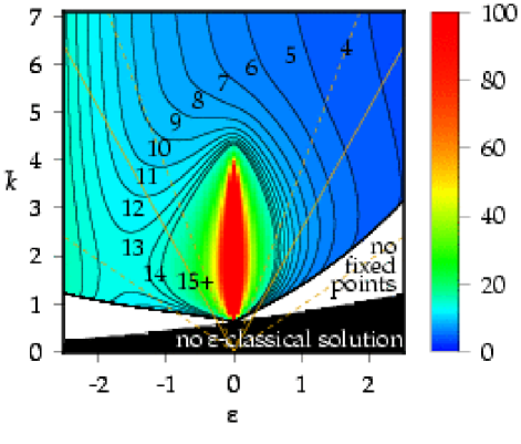
Figure 3: (color online). Number of iterations of Eq. (51) evolved by a Gaussian stable fixed point such that $|\mathcal{J}|<\pi$. Black indicates absence of $\epsilon$-classical stable solutions Fishman2002 , white absence of Gaussian stable solutions. Numbers label the contours where $|\mathcal{J}|<\pi$ for that number of iterations (the number of iterations is capped at 100). The solid line marks the average experimental laser intensity $\phi_{d}=0.8\pi$, dashes demarcate its experimental range ($0.3\pi$–$1.2\pi$) Schlunk2003a . Units are dimensionless.

IV.4 Exact wavepacket dynamics: Comparison

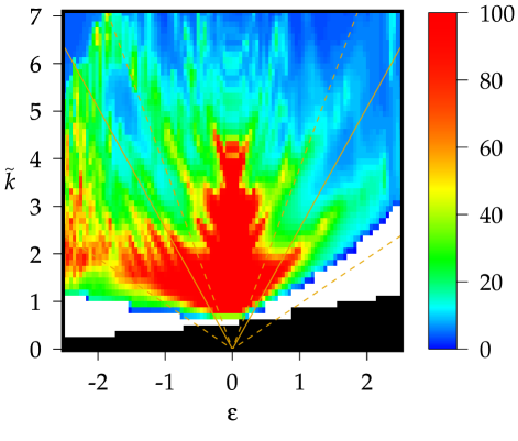
Figure 4: (color online). As in Fig. 3, but for exact wavepacket evolutions, propagating initial conditions from Eq. (67) with the time-evolution operator of Eq. (8) ($\beta=0$). Units are dimensionless.

We now come to the final point of our analysis, propagating Gaussian fixed point solutions using the full second-order cumulant mapping, where all variances must be considered explicitly.

In Fig. 3, we display the time for which the center of mass momentum remains inside its initial phase space cell ($|\mathcal{J}_{n}(\beta)|<\pi$), using this as a rule-of-thumb measure of relative longevity (for a genuine fixed point this would be forever). We see that there is a sizable region where there there are no stable Gaussian fixed points, in addition to the region where there are no $\epsilon$-classical solutions, and that quantum accelerator modes for $\epsilon<0$ are generally more long-lived. These observations are broadly born out by experiment Oberthaler1999 .

We have also computed for how long $|\mathcal{J}_{n}|<\pi$ when integrating the exact evolution described by Eq. (8) dArcy2001 . Due to the fact that we restrict ourselves to a single $\beta$ subspace, the wavefunction we propagate must be a Bloch state, of the form

$$\langle Gz=2\pi l+\theta|\psi\rangle=e^{i\beta(2\pi l+\theta)}\psi(\theta),$$ (65)

which has a discrete momentum spectrum. As we wish to carry out the numerics in the momentum basis, we are therefore obliged for practical reasons to work in the $\hat{\mathcal{I}}(\beta)$ basis rather than that of $\hat{\mathcal{J}}$. The reason is that the spectrum of $\hat{\mathcal{I}}=|\epsilon|\hat{k}$ is fixed, wheras that of $\hat{\mathcal{I}}$ moves with time [see Eq. (33)]. As the discreteness scale is $|\epsilon|$, this issue vanishes in the $\epsilon$-classical limit, but it is unavoidable for any finite value of $\epsilon$ in the fully quantum-mechanical dynamics.

Determining the appropriate initial value for $\tilde{I}(\beta)$ from a predetermined value of $\tilde{\mathcal{J}}$ is, with the aid of the expectation value of Eq. (33), a straightforward matter. The values of $\tilde{\theta}$ and the variances $\tilde{\sigma}^{2}$, $\tilde{\Upsilon}$, and $\tilde{S}^{2}$, are unaffected by this transformation, and so we can set the initial $\psi(\theta)$ to be

$$\begin{split}\psi(\theta,\beta)\propto&[2\pi\tilde{\sigma}^{2}]^{-1/4}\\ &\times\exp\left(-\frac{[1-i2\tilde{\Upsilon}/|\epsilon|][\theta-\tilde{\theta}]^{2}}{4\tilde{\sigma}^{2}}+\frac{i\tilde{\mathcal{I}}(\beta)[\theta-\tilde{\theta}]}{|\epsilon|}\right).\end{split}$$ (66)

The computationally more convenient $\mathcal{I}$ representation of the initial state determined by Eq. (61) is then the discrete Fourier transform of Eq. (66), given by $|\psi\rangle\propto\sum_{n=-\infty}^{\infty}c_{n}|\mathcal{I}=n|\epsilon|\rangle$, where

$$\begin{split}c_{n}=&\left[\frac{\tilde{\sigma}^{2}}{2\pi(\epsilon^{2}/4+\tilde{\Upsilon}^{2})}\right]^{1/4}\\ &\times\exp\left(-\frac{\tilde{\sigma}^{2}/\epsilon^{2}[n|\epsilon|-\tilde{\mathcal{I}}(\beta)]^{2}}{1-i2\tilde{\Upsilon}/|\epsilon|}-\frac{i\tilde{\theta}[n|\epsilon|-\tilde{\mathcal{I}}(\beta)]}{|\epsilon|}\right).\end{split}$$ (67)

This must in principle be normalized numerically, although for a Gaussian state which is well localized in $\theta$, i.e., one where $\sqrt{\sigma^{2}}\ll 2\pi$, the effect of this will be negligible.

Figure 4 shows the results of these integrations. We see that Fig. 3 reproduces its qualitative features quite well, especially for smaller values of $\epsilon$ and $\tilde{k}$. More surprising is the replication of a saddle-point feature at around $\{\epsilon=-1.5,\tilde{k}=2\}$, indicating a resurgence of stability for large $\epsilon$ that is clearly not an artefact of our approximations.

V Conclusions

In conclusion, we have developed a general method for using second order cumulants to study semiclassical-like dynamics near stable periodic orbits in phase space. We have successfully applied this method to quantum accelerator mode dynamics, which operate in an unusual $\epsilon$-semiclassical regime, thus gaining insight into the longevity of quantum accelerator modes in different parameter regimes. We have explictly determined the second-order cumulant mapping for the dynamics of the quantum $\delta$-kicked accelerator, taking place near integer multiples of the the half-Talbot time. In the process, we have shown the $\epsilon$-classical dynamics derived by Fishman, Guarneri, and Rebuzzini, to be the first order approximation within the relevant cumulant hierarchy, we have explained why this description remains effective even for non-negligible values of $\epsilon$, when describing quantum accelerator mode dynamics, and we have shown why, as quantum accelerator modes are traced back to stable periodic orbits in the relevant phase space, our methodology is particularly well suited for analyzing quantum acclerator mode dynamics.

Appendix A Connection between $\epsilon\rightarrow 0$ and the conventional semiclassical limit

From Eq. (5), the Heisenberg equations of motion for $\hat{z}$ and $\hat{p}$ can be determined directly, and integrated to produce the following operator-valued kick-to-kick map:

$$\hat{z}_{n+1}= \hat{z}_{n}+\frac{T}{m}\hat{p}_{n+1}-\frac{gGT^{2}}{2},$$ (68a)

$$\hat{p}_{n+1}= \hat{p}_{n}-G\hbar\phi_{d}\sin(G\hat{z}_{n})+mgT.$$ (68b)

In order to reduce the number of free parameters to a minimum, we rescale the dynamical variables to be dimensionless, such that $\hat{\chi}=G\hat{z}$ and $\hat{\rho}=GT\hat{p}/m$. This produces, from Eq. (68) dArcy2001 ; NoteMap ,

$$\hat{\chi}_{n+1}= \hat{\chi}_{n}+\hat{\rho}_{n+1}+\pi\Omega,$$ (69a)

$$\hat{\rho}_{n+1}= \hat{\rho}_{n}-\kappa\sin\hat{\chi}_{n}-2\pi\Omega,$$ (69b)

where $\kappa=G^{2}T\hbar\phi_{d}/m$ is the usual dimensionless stochasticity parameter associated with the (gravity-free) classical $\delta$-kicked rotor Lichtenberg1992 , and, as elsewhere in this paper, $2\pi\Omega=gG^{2}T$ is a dimensionless parameter quantifying the effect of gravity.

The conventional semiclassical limit of these equations can be achieved by replacing the operator-valued dynamical variables, $\hat{\chi}$ and $\hat{\rho}$, with their expectation values, $\chi=\langle\hat{\chi}\rangle$ and $\rho=\langle\hat{\rho}\rangle$. As explained in Section IV.1, this must coincide with the vanishing of the commutator

$$-i[\hat{\chi},\hat{\rho}]={\mathchoice{\hbox{\raise 5.06941pt\hbox to0.0pt{\kern 1.3802pt\vrule width=2.76042pt,height=0.1pt,depth=0.1pt\hss}\hbox{$\displaystyle k$}}}{\hbox{\raise 5.06941pt\hbox to0.0pt{\kern 1.3802pt\vrule width=2.76042pt,height=0.1pt,depth=0.1pt\hss}\hbox{$\textstyle k$}}}{\hbox{\raise 3.54857pt\hbox to0.0pt{\kern 0.96614pt\vrule width=1.93228pt,height=0.1pt,depth=0.1pt\hss}\hbox{$\scriptstyle k$}}}{\hbox{\raise 2.5347pt\hbox to0.0pt{\kern 0.6901pt\vrule width=1.3802pt,height=0.1pt,depth=0.1pt\hss}\hbox{$\scriptscriptstyle k$}}}}=\frac{\hbar G^{2}T}{m}=\frac{2\pi T}{T_{1/2}},$$ (70)

where $T_{1/2}=2\pi m/\hbar G^{2}$ is the half-Talbot time.

The scaled Planck constant  $\textstyle k$ is that conventionally used in studies of $\delta$-kicked rotor/particle dynamics, particularly when investigating the semiclassical limit, defined as ${\mathchoice{\hbox{\raise 5.06941pt\hbox to0.0pt{\kern 1.3802pt\vrule width=2.76042pt,height=0.1pt,depth=0.1pt\hss}\hbox{$\displaystyle k$}}}{\hbox{\raise 5.06941pt\hbox to0.0pt{\kern 1.3802pt\vrule width=2.76042pt,height=0.1pt,depth=0.1pt\hss}\hbox{$\textstyle k$}}}{\hbox{\raise 3.54857pt\hbox to0.0pt{\kern 0.96614pt\vrule width=1.93228pt,height=0.1pt,depth=0.1pt\hss}\hbox{$\scriptstyle k$}}}{\hbox{\raise 2.5347pt\hbox to0.0pt{\kern 0.6901pt\vrule width=1.3802pt,height=0.1pt,depth=0.1pt\hss}\hbox{$\scriptscriptstyle k$}}}}\rightarrow 0$ Klappauf1998 . We recall that the smallness parameter $\epsilon$ upon which the concept of $\epsilon$ classics and semiclassics in this Paper is based, is defined within

$$T=(2\pi\ell+\epsilon)\frac{m}{\hbar G^{2}}=T_{1/2}\left(\ell+\frac{\epsilon}{2\pi}\right),$$ (71)

where $\ell\in\mathbb{Z}$. Substituting Eq. (71) into Eq. (70), we therefore get

$${\mathchoice{\hbox{\raise 5.06941pt\hbox to0.0pt{\kern 1.3802pt\vrule width=2.76042pt,height=0.1pt,depth=0.1pt\hss}\hbox{$\displaystyle k$}}}{\hbox{\raise 5.06941pt\hbox to0.0pt{\kern 1.3802pt\vrule width=2.76042pt,height=0.1pt,depth=0.1pt\hss}\hbox{$\textstyle k$}}}{\hbox{\raise 3.54857pt\hbox to0.0pt{\kern 0.96614pt\vrule width=1.93228pt,height=0.1pt,depth=0.1pt\hss}\hbox{$\scriptstyle k$}}}{\hbox{\raise 2.5347pt\hbox to0.0pt{\kern 0.6901pt\vrule width=1.3802pt,height=0.1pt,depth=0.1pt\hss}\hbox{$\scriptscriptstyle k$}}}}=2\pi\ell+\epsilon,$$ (72)

and we see that taking the $\epsilon$-classical limit is equivalent to the conventional rescaled Planck constant  $\textstyle k$ being equal to an integer multiple of $2\pi$.

Appendix B Bloch parametrization of the dynamical variables

B.1 Overview

We will now explore some relevant details of our chosen parametrization of the position and momentum variables, formulating inner products, operators, and commutation relations in terms of the angle $\theta$, the quasimomentum $\beta$, the discrete position $l$, and the discrete momentum $k$.

B.2 Inner products

We define

$$\langle Gz=2\pi l+\theta|(\hbar G)^{-1}p=k+\beta\rangle=\frac{1}{\sqrt{2\pi}}e^{i(\beta\theta+\beta 2\pi l+k\theta)}$$ (73)

and, bearing in mind the limited ranges of $\theta\in[0,2\pi)$ and $\beta\in[0,1)$, note the following identities:

$$\sum_{k=-\infty}^{\infty}e^{-ik(\theta-\theta^{\prime})}= 2\pi\delta(\theta-\theta^{\prime}),$$ (74)

$$\int d\theta e^{i\theta(k-k^{\prime})}= 2\pi\delta_{kk^{\prime}},$$ (75)

$$\sum_{l=-\infty}^{\infty}e^{-i2\pi l(\beta-\beta^{\prime})}= \delta(\beta-\beta^{\prime}),$$ (76)

$$\int d\beta e^{i\beta 2\pi(l-l^{\prime})}= \delta_{ll^{\prime}}.$$ (77)

Inserting the position representation of the identity operator into the inner product $\langle Gz=2\pi l+\theta|Gz=2\pi l^{\prime}+\theta^{\prime}\rangle$ we find, using Eq. (73), that

$$\begin{split}\langle Gz=2\pi l+\theta|Gz=2\pi l^{\prime}+\theta^{\prime}\rangle=&\int d\beta e^{i\beta 2\pi(l-l^{\prime})}e^{i\beta(\theta-\theta^{\prime})}\\ &\times\frac{1}{2\pi}\sum_{k=-\infty}^{\infty}e^{ik(\theta-\theta^{\prime})}.\end{split}$$ (78)

Substituting Eq. (74) into Eq. (78), it simplifies to

$$\langle Gz=2\pi l+\theta|Gz=2\pi l^{\prime}+\theta^{\prime}\rangle=\int d\beta e^{i\beta 2\pi(l-l^{\prime})}\delta(\theta-\theta^{\prime}),$$ (79)

which, with the aid of Eq. (75), results in the following general form for the inner product of two rescaled position eigenstates, in terms of the angle $\theta$ and the discrete position variable $l$:

$$\langle Gz=2\pi l+\theta|Gz=2\pi l^{\prime}+\theta^{\prime}\rangle=\delta_{ll^{\prime}}\delta(\theta-\theta^{\prime}).$$ (80)

Similarly, using Eqs. (76) and (77), one can straightforwardly determine a corresponding expression for the inner product of two rescaled momentum eigenstates, in terms of the quasimomentum $\beta$ and the discrete momentum $k$:

$$\langle(\hbar G)^{-1}p=k+\beta|(\hbar G)^{-1}p=k^{\prime}+\beta^{\prime}\rangle=\delta_{kk^{\prime}}\delta(\beta-\beta^{\prime}).$$ (81)

B.3 Operators

Having determined all the relevant inner products in terms of $\theta$, $l$, $\beta$, and $k$, we set

$$\hat{l}= \int d\theta\sum_{l=-\infty}^{\infty}|Gz=2\pi l+\theta\rangle l\langle Gz=2\pi l+\theta|,$$ (82)

$$\hat{\theta}= \int d\theta\sum_{l=-\infty}^{\infty}|Gz=2\pi l+\theta\rangle\theta\langle Gz=2\pi l+\theta|,$$ (83)

$$\hat{k}= \int d\beta\sum_{k=-\infty}^{\infty}|(\hbar G)^{-1}p=k+\beta\rangle k\langle(\hbar G)^{-1}p=k+\beta|,$$ (84)

$$\hat{\beta}= \int d\beta\sum_{k=-\infty}^{\infty}|(\hbar G)^{-1}p=k+\beta\rangle\beta\langle(\hbar G)^{-1}p=k+\beta|.$$ (85)

These operators are defined such that $\hat{l}|Gz=2\pi l+\theta\rangle=l|Gz=2\pi l+\theta\rangle$, $\hat{\theta}|Gz=2\pi l+\theta\rangle=\theta|Gz=2\pi l+\theta\rangle$, $\hat{k}|(\hbar G)^{-1}p=k+\beta\rangle=k|(\hbar G)^{-1}p=k+\beta\rangle$, and $\hat{\beta}|(\hbar G)^{-1}p=k+\beta\rangle=\beta|(\hbar G)^{-1}p=k+\beta\rangle$, as can readily be confirmed with the aid of Eqs. (80) and (81). In addition, clearly

$$\hat{\theta}+2\pi\hat{l}= G\hat{z},$$ (86)

$$\hat{\beta}+\hat{k}= \frac{\hat{p}}{\hbar G}.$$ (87)

B.4 Commutators

We now determine the commutators of the various parametrized position and momentum dynamical variables.

We begin by considering the angle $\hat{\theta}$, and the quasimomentum $\hat{\beta}$. Using Eqs. (83), (85), and (73), we readily determine that

$$\begin{split}\hat{\beta}\hat{\theta}=&\frac{1}{\sqrt{2\pi}}\iint d\beta d\theta\beta\theta e^{-i\theta\beta}\\ &\times\sum_{k,l=-\infty}^{\infty}|(\hbar G)^{-1}p=k+\beta\rangle e^{-i(\theta k+2\pi l\beta)}\langle Gz=2\pi l+\theta|.\end{split}$$ (88)

Sandwiching this expression between identity operators, in the position and momentum representations, respectively, produces, with the aid of Eqs. (73), (74), and (76),

$$\begin{split}\hat{\beta}\hat{\theta}=&\frac{1}{\sqrt{2\pi}}\iint d\beta d\theta\beta\theta e^{i\theta\beta}\\ &\times\sum_{k^{\prime},l^{\prime}=-\infty}^{\infty}|(\hbar G)^{-1}p=k+\beta\rangle e^{i\theta k^{\prime}}e^{i2\pi l^{\prime}\beta}\langle Gz=2\pi l+\theta|\\ =&(\hat{\beta}\hat{\theta})^{\dagger}\\ =&\hat{\theta}\hat{\beta}.\end{split}$$ (89)

It therefore follows that the quasimomentum and angle operators commute, i.e.,

$$[\hat{\theta},\hat{\beta}]=0.$$ (90)

Considering now the discrete momentum $\hat{k}$ and the angle $\hat{\theta}$, we determine, from Eqs.  (73), (83), and (84), that

$$\begin{split}\hat{k}\hat{\theta}=&\frac{1}{\sqrt{2\pi}}\int d\theta\sum_{k=-\infty}^{\infty}k\theta e^{-i\theta k}\\ &\times\int d\beta\sum_{l=-\infty}^{\infty}|(\hbar G)^{-1}p=k+\beta\rangle e^{-i(\theta k+2\pi l\beta)}\langle Gz=2\pi l+\theta|.\end{split}$$ (91)

In analogous fashion to what was carried out for the $\hat{\beta}\hat{\theta}$ product, we sandwich this expression between identity operators in the position and momentum representations, respectively, producing with the aid of Eq. (73):

$$\begin{split}\hat{k}\hat{\theta}=&\frac{1}{\sqrt{2\pi}}\iint d\beta^{\prime}d\theta^{\prime}\sum_{k^{\prime},l^{\prime}=-\infty}^{\infty}|(\hbar G)^{-1}p=k^{\prime}+\beta^{\prime}\rangle\\ &\times\frac{1}{2\pi}e^{i[\beta^{\prime}(\theta^{\prime}+2\pi l^{\prime})]}\int d\theta\theta e^{ik^{\prime}\theta}\sum_{k=-\infty}^{\infty}ke^{ik(\theta^{\prime}-\theta)}\\ &\times\langle Gz=2\pi l^{\prime}+\theta^{\prime}|.\end{split}$$ (92)

We now use the identity Cohen1977

$$\int d\theta f(\theta)\frac{\partial}{\partial\theta^{\prime}}\delta(\theta-\theta^{\prime})=\frac{\partial}{\partial\theta^{\prime}}f(\theta^{\prime})$$ (93)

along with Eq. (74) to determine that

$$\begin{split}\int d\theta\theta e^{ik^{\prime}\theta}\sum_{k=-\infty}^{\infty}ke^{ik(\theta^{\prime}-\theta)}=&\int d\theta\theta e^{ik^{\prime}\theta}\left[-i\frac{\partial}{\partial\theta^{\prime}}\sum_{k=-\infty}^{\infty}e^{ik(\theta^{\prime}-\theta)}\right]\\ =&-i2\pi\int d\theta\theta e^{ik^{\prime}\theta}\frac{\partial}{\partial\theta^{\prime}}\delta(\theta-\theta^{\prime})\\ =&2\pi(\theta^{\prime}k^{\prime}-i)e^{ik^{\prime}\theta^{\prime}},\end{split}$$ (94)

and insert this expression back into Eq. (92), to reveal

$$\hat{k}\hat{\theta}=(\hat{k}\hat{\theta})^{\dagger}-i=\hat{\theta}\hat{k}-i,$$ (95)

which result is more conveniently phrased within the commutator

$$[\hat{\theta},\hat{k}]=i.$$ (96)

In a very similar manner, using Eq. (76) and inserting a partial derivative with respect to the quasimomentum $\beta$, it can be shown that $2\pi\hat{l}\hat{\beta}=(2\pi\hat{l}\hat{\beta})^{\dagger}+i$, and therefore that

$$[\hat{l},\hat{\beta}]=\frac{i}{2\pi}.$$ (97)

Referring to Eqs. (86) and (87), we can now deduce from $[\hat{z},\hat{p}]/\hbar=[\hat{\theta},\hat{\beta}]+[\hat{\theta},\hat{k}]+2\pi([\hat{l},\hat{\beta}]+[\hat{l},\hat{k}])=i$ that

$$[\hat{k},\hat{l}]=\frac{i}{2\pi}.$$ (98)

Trivially, $[\hat{\theta},\hat{l}]=[\hat{k},\hat{\beta}]=0$, and so, to summarize:

$$[\hat{\theta},\hat{k}]=i,$$ (99)

$$[\hat{k},\hat{l}]=[\hat{l},\hat{\beta}]=\frac{i}{2\pi},$$ (100)

$$[\hat{\theta},\hat{\beta}]=[\hat{\theta},\hat{l}]=[\hat{k},\hat{\beta}]=0.$$ (101)

Appendix C Second-order cumulants

C.1 Counting statistics

We choose to approximately express a given order $2n$ moment $\langle\hat{q}_{1}\hat{q}_{2}\ldots\hat{q}_{2n}\rangle$ in terms of first and second order cumulants only, i.e., means and variances, setting third- and higher-order cumulants to zero [see Eq. (4)]. The moment can be expressed as a sum of $n$ terms, each consisting of a product of $k$ variances and $2(n-k)$ means.

Taking one such term, when considering how many ways there are to produce a product of $k$ variances and $2(n-k)$ means, this is equivalent to determining how many ways there are to partition the $\hat{q}_{i}$ terms into two subsets, one with $2k$ elements which pairwise form variances, and the other with $2(n-k)$ elements individually forming means.

Our starting point is to consider all possible permutations (i.e., orderings) of the $\hat{q}_{i}$ terms. For $n=3$ one possible permutation is

$$\hat{q}_{3}\hat{q}_{1}\hat{q}_{6}\hat{q}_{2}\hat{q}_{4}\hat{q}_{5}.$$ (102)

The first $2k$ terms in the permutation are partitioned into unique neighbouring pairs, and all subsequent terms are are partitioned into individual units, e.g. for $n=4$, $k=2$ and this permutation

$$\langle\langle\hat{q}_{3}\hat{q}_{1}\rangle\rangle\langle\langle\hat{q}_{6}\hat{q}_{2}\rangle\rangle\langle\langle\hat{q}_{4}\rangle\rangle\langle\langle\hat{q}_{5}\rangle\rangle.$$ (103)

We thus have $k$ pairs, identified with variances, and $2(n-k)$ individual terms, identified with means. There are $(2n)!$ such permutations.

As there is only one “correct” ordering, set by the ordering of the operators in the original moment, we must correct for overcounting. In particular the “correct” ordering of the operators making up the variances is in ascending order of the value of the subscript. The ordering of the individual means and variances with respect to each other is obviously unimportant. The complete set of equivalent orderings is thus:

$$\begin{split}&\left\{\langle\langle\hat{q}_{1}\hat{q}_{3}\rangle\rangle\langle\langle\hat{q}_{2}\hat{q}_{6}\rangle\rangle\langle\langle\hat{q}_{4}\rangle\rangle\langle\langle\hat{q}_{5}\rangle\rangle,\right.\\ &\langle\langle\hat{q}_{1}\hat{q}_{3}\rangle\rangle\langle\langle\hat{q}_{2}\hat{q}_{6}\rangle\rangle\langle\langle\hat{q}_{5}\rangle\rangle\langle\langle\hat{q}_{4}\rangle\rangle,\\ &\langle\langle\hat{q}_{2}\hat{q}_{6}\rangle\rangle\langle\langle\hat{q}_{1}\hat{q}_{3}\rangle\rangle\langle\langle\hat{q}_{4}\rangle\rangle\langle\langle\hat{q}_{5}\rangle\rangle,\\ &\langle\langle\hat{q}_{2}\hat{q}_{6}\rangle\rangle\langle\langle\hat{q}_{1}\hat{q}_{3}\rangle\rangle\langle\langle\hat{q}_{5}\rangle\rangle\langle\langle\hat{q}_{4}\rangle\rangle,\\ &\langle\langle\hat{q}_{3}\hat{q}_{1}\rangle\rangle\langle\langle\hat{q}_{2}\hat{q}_{6}\rangle\rangle\langle\langle\hat{q}_{4}\rangle\rangle\langle\langle\hat{q}_{5}\rangle\rangle,\\ &\langle\langle\hat{q}_{3}\hat{q}_{1}\rangle\rangle\langle\langle\hat{q}_{2}\hat{q}_{6}\rangle\rangle\langle\langle\hat{q}_{5}\rangle\rangle\langle\langle\hat{q}_{4}\rangle\rangle,\\ &\langle\langle\hat{q}_{2}\hat{q}_{6}\rangle\rangle\langle\langle\hat{q}_{3}\hat{q}_{1}\rangle\rangle\langle\langle\hat{q}_{4}\rangle\rangle\langle\langle\hat{q}_{5}\rangle\rangle,\\ &\langle\langle\hat{q}_{2}\hat{q}_{6}\rangle\rangle\langle\langle\hat{q}_{3}\hat{q}_{1}\rangle\rangle\langle\langle\hat{q}_{5}\rangle\rangle\langle\langle\hat{q}_{4}\rangle\rangle,\\ &\langle\langle\hat{q}_{1}\hat{q}_{3}\rangle\rangle\langle\langle\hat{q}_{6}\hat{q}_{2}\rangle\rangle\langle\langle\hat{q}_{4}\rangle\rangle\langle\langle\hat{q}_{5}\rangle\rangle,\\ &\langle\langle\hat{q}_{1}\hat{q}_{3}\rangle\rangle\langle\langle\hat{q}_{6}\hat{q}_{2}\rangle\rangle\langle\langle\hat{q}_{5}\rangle\rangle\langle\langle\hat{q}_{4}\rangle\rangle,\\ &\langle\langle\hat{q}_{6}\hat{q}_{2}\rangle\rangle\langle\langle\hat{q}_{1}\hat{q}_{3}\rangle\rangle\langle\langle\hat{q}_{4}\rangle\rangle\langle\langle\hat{q}_{5}\rangle\rangle,\\ &\langle\langle\hat{q}_{6}\hat{q}_{2}\rangle\rangle\langle\langle\hat{q}_{1}\hat{q}_{3}\rangle\rangle\langle\langle\hat{q}_{5}\rangle\rangle\langle\langle\hat{q}_{4}\rangle\rangle,\\ &\langle\langle\hat{q}_{3}\hat{q}_{1}\rangle\rangle\langle\langle\hat{q}_{6}\hat{q}_{2}\rangle\rangle\langle\langle\hat{q}_{4}\rangle\rangle\langle\langle\hat{q}_{5}\rangle\rangle,\\ &\langle\langle\hat{q}_{3}\hat{q}_{1}\rangle\rangle\langle\langle\hat{q}_{6}\hat{q}_{2}\rangle\rangle\langle\langle\hat{q}_{5}\rangle\rangle\langle\langle\hat{q}_{4}\rangle\rangle,\\ &\langle\langle\hat{q}_{6}\hat{q}_{6}\rangle\rangle\langle\langle\hat{q}_{3}\hat{q}_{1}\rangle\rangle\langle\langle\hat{q}_{4}\rangle\rangle\langle\langle\hat{q}_{5}\rangle\rangle,\\ &\left.\langle\langle\hat{q}_{6}\hat{q}_{2}\rangle\rangle\langle\langle\hat{q}_{3}\hat{q}_{1}\rangle\rangle\langle\langle\hat{q}_{5}\rangle\rangle\langle\langle\hat{q}_{4}\rangle\rangle\right\}.\end{split}$$ (104)

In general there are $k!$ (all the possible orderings of the variances) multiplied by $2^{k}$ (all the possible operator orderings within the variances to the power of the number of variances) multiplied by $[2(n-k)]!$ (all the possible orderings of the means) equivalent possibilities. Only one should be counted.

C.2 General expansions of moments in means and variances

If the $\hat{q}_{i}$ are identical, then, designating the mean $\langle\langle\hat{q}\rangle\rangle=\langle\hat{q}\rangle=\mu$ and variance $\langle\langle\hat{q}^{2}\rangle\rangle=\langle\hat{q}^{2}\rangle-\langle\hat{q}\rangle^{2}=\sigma^{2}$, we can determine an approximate expression for the moment $\langle\hat{q}^{2n}\rangle$ purely in terms of $\mu_{q}$ and $\sigma_{q}^{2}$:

$$\langle\hat{q}^{2n}\rangle\simeq\sum_{k=0}^{n}\frac{(2n)!}{[2(n-k)]!k!2^{k}}\mu^{2(n-k)}(\sigma^{2})^{k}.$$ (105)

For a general order $2n+1$ moment, the corresponding approximate expression is given by:

$$\langle\hat{q}^{2n+1}\rangle\simeq\sum_{k=0}^{n}\frac{(2n+1)!}{[2(n-k)+1]!k!2^{k}}\mu^{2(n-k)+1}(\sigma^{2})^{k}.$$ (106)

If we consider the expectation value of an averaged symmetrized sum of products of a separately considered operator $\hat{q}_{1}$ with a product of identical operators $\hat{q}_{2}$, i.e., $\langle\hat{q}_{1}\hat{q}_{2}^{2n}+\hat{q}_{2}^{2n}\hat{q}_{1}\rangle/2$, then Eqs. (105) and (106) can be combined to produce a similar approximate expression:

$$\begin{split}\frac{1}{2}\langle\hat{q}_{1}\hat{q}_{2}^{2n}+\hat{q}_{2}^{2n}\hat{q}_{1}\rangle\simeq&\mu_{1}\sum_{k=0}^{n}\frac{(2n)!}{[2(n-k)]!k!2^{k}}\mu_{2}^{2(n-k)}(\sigma_{2}^{2})^{k}\\ &+2n\sigma_{12}^{2}\sum_{k=0}^{n-1}\frac{(2n-1)!}{[2(n-k)-1]!k!2^{k}}\\ &\times\mu_{2}^{2(n-k)-1}(\sigma_{2}^{2})^{k},\end{split}$$ (107)

where $\mu_{1}=\langle\hat{q}_{1}\rangle$ and $\mu_{2}=\langle\hat{q}_{2}\rangle$ are means, $\sigma_{2}=\langle\hat{q}_{2}^{2}\rangle-\langle\hat{q}_{2}\rangle^{2}$ is a variance, and $\sigma_{12}=\langle\hat{q}_{1}\hat{q}_{2}+\hat{q}_{2}\hat{q}_{1}\rangle/2-\langle\hat{q}_{1}\rangle\langle\hat{q}_{2}\rangle$ is a symmetrized covariance. Similarly, for an equivalent symmetrized moment containing odd powers of $\hat{q}_{2}$,

$$\begin{split}\frac{1}{2}\langle\hat{q}_{1}\hat{q}_{2}^{2n+1}+\hat{q}_{2}^{2n+1}\hat{q}_{1}\rangle\simeq&\mu_{1}\sum_{k=0}^{n}\frac{(2n+1)!}{[2(n-k)+1]!k!2^{k}}\\ &\times\mu_{2}^{2(n-k)+1}(\sigma_{2}^{2})^{k}\\ &+(2n+1)\sigma_{12}^{2}\sum_{k=0}^{n}\frac{(2n)!}{[2(n-k)]!k!2^{k}}\\ &\times\mu_{2}^{2(n-k)}(\sigma_{2}^{2})^{k}.\end{split}$$ (108)

Drawing on Eq. (105) it is now straightforward to approximately expand the expectation value of the cosine of an operator in terms of means and variances:

$$\begin{split}\langle\cos\hat{q}\rangle=&\sum_{n=0}^{\infty}\frac{(-1)^{n}}{(2n)!}\langle\hat{q}^{2n}\rangle\\ \simeq&\sum_{n=0}^{\infty}\frac{(-1)^{n}}{(2n)!}\sum_{k=0}^{n}\frac{(2n)!}{[2(n-k)]!k!2^{k}}\mu^{2(n-k)}(\sigma^{2})^{k}\\ =&\sum_{k=0}^{\infty}\sum_{n=k}^{\infty}\frac{(-1)^{n}}{[2(n-k)]!k!}\mu^{2(n-k)}(\sigma^{2}/2)^{k}\\ =&\sum_{k=0}^{\infty}\sum_{l=0}^{\infty}\frac{(-1)^{l+k}}{(2l)!k!}\mu^{2l}(\sigma^{2}/2)^{k}\\ =&\sum_{k=0}^{\infty}\frac{(-\sigma^{2}/2)^{k}}{k!}\sum_{l=0}^{\infty}\frac{(-1)^{l}}{(2l)!}\mu^{2l}\\ =&e^{-\sigma^{2}/2}\cos\mu.\end{split}$$ (109)

One can similarly draw on Eq. (106) to carry out an equivalent expansion for the expectation value of the sine of an operator:

$$\begin{split}\langle\sin\hat{q}\rangle=&\sum_{n=0}^{\infty}\frac{(-1)^{n}}{(2n+1)!}\langle\hat{q}^{2n+1}\rangle\\ \simeq&\sum_{k=0}^{\infty}\sum_{n=k}^{\infty}\frac{(-1)^{n}}{[2(n-k)+1]!k!}\mu^{2(n-k)+1}(\sigma^{2}/2)^{k}\\ =&\sum_{k=0}^{\infty}\sum_{l=0}^{\infty}\frac{(-1)^{l+k}}{(2l+1)!k!}\mu^{2l+1}(\sigma^{2}/2)^{k}\\ =&e^{-\sigma^{2}/2}\sin\mu.\end{split}$$ (110)

Finally, by making use of Eq. (108), one can straightforwardly determine an approximate expansion of the expectation value of an averaged symmetrized sum of products of the the sine of one operator multiplied by a second operator, in terms of means and variances:

$$\begin{split}\frac{1}{2}\langle\hat{q}_{1}\sin\hat{q}_{2}+(\sin\hat{q}_{2})\hat{q}_{1}\rangle=&\sum_{n=0}^{\infty}\frac{(-1)^{n}}{(2n+1)!}\frac{1}{2}\langle\hat{q}_{1}\hat{q}_{2}^{2n+1}+\hat{q}_{2}^{2n+1}\hat{q}_{1}\rangle\\ \simeq&\sum_{n=0}^{\infty}\frac{(-1)^{n}}{(2n+1)!}\sum_{k=0}^{n}\left\{\mu_{1}\frac{(2n+1)!}{[2(n-k)+1]!k!2^{k}}\mu_{2}^{2(n-k)+1}(\sigma_{2}^{2})^{k}+\sigma_{12}^{2}\frac{(2n+1)!}{[2(n-k)]!k!2^{k}}\mu_{2}^{2(n-k)}(\sigma_{2}^{2})^{k}\right\}\\ =&\sum_{k=0}^{\infty}\sum_{k=n}^{\infty}\left\{\mu_{1}\frac{(-1)^{n}}{[2(n-k)+1]!k!}\mu_{2}^{2(n-k)+1}(\sigma_{2}^{2}/2)^{k}+\sigma_{12}^{2}\frac{(-1)^{n}}{[2(n-k)]!k!}\mu_{2}^{2(n-k)}(\sigma_{2}^{2}/2)^{k}\right\}\\ =&\sum_{k=0}^{\infty}\frac{(-1)^{k}}{k!}(\sigma_{2}^{2}/2)^{k}\left\{\mu_{1}\sum_{l=0}^{\infty}\frac{(-1)^{l}}{(2l+1)!}\mu_{2}^{2l+1}+\sigma_{12}^{2}\sum_{l=0}^{\infty}\frac{(-1)^{l}}{(2l)!}\mu_{2}^{2l}\right\}\\ =&e^{-\sigma_{2}^{2}/2}(\mu_{1}\sin\mu_{2}+\sigma_{12}^{2}\cos\mu_{2}).\end{split}$$ (111)

With these identities we now have everything necessary to determine the second-order cumulant dynamics quantum accelerator modes in the $\delta$-kicked accelerator.

C.3 Formulation of expansions relevant to quantum accelerator mode dynamics

The dynamical variables relevant to $\delta$-kicked accelerator and quantum accelerator mode dynamics are $\hat{\theta}$ and $\hat{\mathcal{J}}$. All expectation values are evaluated within a reduced subspace particular to a specific value of the quasimomentum $\beta$, only, as detailed in Section III.2.6.

Bearing this in mind, we determine from Eq. (110) that

$$\langle\sin\hat{\theta}\rangle(\beta)=e^{-\sigma^{2}(\beta)/2}\sin\theta(\beta).$$ (112)

Using Eq. (109), we determine that

$$\langle\cos\hat{\theta}\rangle(\beta)=e^{-\sigma^{2}(\beta)/2}\cos\theta(\beta),$$ (113)

and that

$$\begin{split}\langle\sin^{2}\hat{\theta}\rangle(\beta)=&\frac{1}{2}[1-\langle\cos(2\hat{\theta})\rangle(\beta)]\\ =&\frac{1}{2}\{1-e^{-2\sigma^{2}(\beta)}\cos[2\theta(\beta)]\}.\end{split}$$ (114)

Using Eq. (111), we straightforwardly determine that

$$\begin{split}\frac{1}{2}\langle\hat{\mathcal{J}}\sin\hat{\theta}+(\sin\hat{\theta})\hat{\mathcal{J}}\rangle(\beta)=&e^{-\sigma^{2}(\beta)/2}\mathcal{J}(\beta)\sin\theta(\beta)\\ &+e^{-\sigma^{2}(\beta)/2}\Upsilon(\beta)\cos\theta(\beta),\end{split}$$ (115)

and, again by using Eq. (111), where we set $\hat{q}_{1}=\hat{q}_{2}$, we determine that

$$\langle\hat{\theta}\sin\hat{\theta}\rangle(\beta)=e^{-\sigma^{2}(\beta)/2}[\theta(\beta)\sin\theta(\beta)+\sigma^{2}(\beta)\cos\theta(\beta)].$$ (116)

Appendix D Analogy: $\beta$-rotors

D.1 Overview

Subspaces of different $\beta$ (in an accelerating frame) are decoupled in $\delta$-kicked accelerator dynamics. A wavefunction contained within any such subspace is periodic, multiplied by a quasimomentum and position dependent phase $e^{-i\beta Gx}$, and can be equivalently represented by a rotor wavefunction. We will now discuss the connection in some detail, in particular so as to more explicitly link the operator oriented formalism used in this paper with the $\beta$-rotor picture used originally by Fishman, Guarneri, and Rebuzzini Fishman2002 .

D.2 Density operator

We consider an assumed well defined and unit trace density operator, which, in the momentum representation, has the general form

$$\begin{split}\rho=&\iint d\beta d\beta^{\prime}\sum_{k,k^{\prime}=-\infty}^{\infty}d_{kk^{\prime}}(\beta,\beta^{\prime})\\ &\times|(\hbar G)^{-1}p=k+\beta\rangle\langle(\hbar G)^{-1}p=k^{\prime}+\beta^{\prime}|.\end{split}$$ (117)

We select out that part of the density operator specific to a particular $\beta$ subspace by sandwiching it between $\beta$-specific projection operators $\hat{\mathcal{P}}(\beta)$, as defined in Eq. (28). The resulting expression is given by

$$\begin{split}\hat{\mathcal{P}}(\beta)\rho\hat{\mathcal{P}}(\beta)=&\iint d\beta^{\prime\prime}d\beta^{\prime\prime\prime}\sum_{k,k^{\prime},k^{\prime\prime},k^{\prime\prime\prime}=-\infty}^{\infty}\delta_{k^{\prime}k^{\prime\prime}}\delta(\beta-\beta^{\prime\prime})\\ &\times d_{k^{\prime\prime}k^{\prime\prime\prime}}(\beta^{\prime\prime},\beta^{\prime\prime\prime})\delta_{k^{\prime\prime\prime}k^{\prime}}\delta(\beta^{\prime\prime\prime}-\beta)\\ &\times|(\hbar G)^{-1}p=k+\beta\rangle\langle(\hbar G)^{-1}p=k^{\prime}+\beta|\\ =&\sum_{k,k^{\prime}=-\infty}^{\infty}d_{kk^{\prime}}(\beta,\beta)\\ &\times|(\hbar G)^{-1}p=k+\beta\rangle\langle(\hbar G)^{-1}p=k^{\prime}+\beta|.\end{split}$$ (118)

A general matrix element of this projected out density operator, in the position representation, is then given by the following inner product:

$$\begin{split}\sum_{k,k^{\prime}=-\infty}^{\infty}\langle Gz=2\pi l+\theta|(\hbar G)^{-1}p=k+\beta\rangle d_{kk^{\prime}}(\beta,\beta)\langle(\hbar G)^{-1}p=k^{\prime}+\beta|Gz=2\pi l+\theta\rangle&=\varrho(\theta,\theta^{\prime},\beta)e^{i\beta(\theta-\theta^{\prime})}e^{i2\pi(l-l^{\prime})\beta},\end{split}$$ (119)

where

$$\varrho(\theta,\theta^{\prime},\beta)=\sum_{k,k^{\prime}}d_{kk^{\prime}}(\beta,\beta)\frac{e^{i(k\theta-k^{\prime}\theta^{\prime})}}{2\pi}.$$ (120)

Just as for plane waves, states resulting from the projection $\hat{\mathcal{P}}(\beta)\rho\hat{\mathcal{P}}(\beta)$ are extended in position space, due to the fact that they are, in general, incoherent superpositions of Bloch states for one particular value of the quasimomentum $\beta$.

Bloch states are not normalizable (i.e., they lie outside the Hilbert space) when the inner product is defined in the usual way; the trace of the expression Eq. (119), defined as summing and integrating over all terms where $\theta=\theta^{\prime}$ and $l=l^{\prime}$, can be seen to be similarly problematical.

We note, however, that the normalizing factor $\mathcal{N}(\beta)$ defined in Eq. (27) is given by integrating over the diagonal elements of $\varrho(\theta,\theta^{\prime})$ alone, i.e.,

$$\begin{split}\int d\theta\varrho(\theta,\theta,\beta)=&\sum_{kk^{\prime}=-\infty}^{\infty}d_{kk^{\prime}}(\beta,\beta)\int d\theta\frac{e^{i(k-k^{\prime})\theta}}{2\pi}\\ =&\sum_{k=-\infty}^{\infty}d_{kk}(\beta,\beta)\equiv\mathcal{N}(\beta)\end{split}$$ (121)

This takes advantage of the fact that integrating the diagonal matrix elements of Eq. (119) over any length $2\pi$ interval will give the same answer. This is in turn due to the periodic nature of the state, apart from quasimomentum dependent phases, which are in any case absent on the diagonal.

Effectively, if we are restricted to a single $\beta$ subspace, we can define an inner product as the integral over $\theta$ from $a$ to $a+2\pi$, at a particular value of $l$, which can be chosen arbitrarily. This provides a well-defined norm for Bloch states, which have been mapped from the inifinite, continuous position basis appropriate for a free particle, to the periodic position basis appropriate for a rotor.

D.3 Discrete momentum operator

We consider the action of the discrete momentum operator $\hat{k}$ restricted to a particular $\beta$ subspace, i.e., when acting on a projected density operator as defined in Eq. (118).

In the position representation, we end up with the familiar differential operator form appropriate for dynamics occuring on a circle:

$$\begin{split}\langle Gz=2\pi l+\theta|\hat{k}\hat{\mathcal{P}}(\beta)\rho\hat{\mathcal{P}}(\beta)|Gz=2\pi l^{\prime}+\theta^{\prime}\rangle=&e^{i2\pi(l-l^{\prime})\beta}e^{i(\theta-\theta^{\prime})\beta}\frac{1}{2\pi}\sum_{k,k^{\prime}=-\infty}^{\infty}kd_{kk^{\prime}}(\beta,\beta)\\ =&e^{i2\pi(l-l^{\prime})\beta}e^{i(\theta-\theta^{\prime})\beta}\ \left[-i\frac{\partial}{\partial\theta}\varrho(\theta,\theta^{\prime},\beta)\right].\end{split}$$ (122)

Note that the differential operator $-i\partial/\partial\theta$ needs to be taken inside the quasimomentum dependent phases, and thus it acts directly on $\varrho(\theta,\theta^{\prime})$.

D.4 $\beta$-conditional expectation values

D.4.1 Discrete momentum expectation value

The (normalized) expectation value of the discrete momentum operator $\hat{k}$ conditioned to a single value of $\beta$ is given by taking the normalized partial trace, as defined in Eq. (27), of $\hat{k}$ multiplied by the density operator $\rho$, i.e.,

$$\langle\hat{k}\rangle(\beta)=\frac{1}{\mathcal{N}(\beta)}\sum_{k=-\infty}^{\infty}\langle(\hbar G)^{-1}p=k+\beta|\hat{k}\rho|(\hbar G)^{-1}p=k+\beta\rangle.$$ (123)

Inserting the general density operator defined in Eq. (117) produces

$$\langle\hat{k}\rangle(\beta)=\frac{1}{\mathcal{N}(\beta)}\sum_{k=-\infty}^{\infty}kd_{kk}(\beta,\beta).$$ (124)

With the aid of Eq. (120), some fairly elementary manipulations prove this expression to be fully equivalent to

$$\begin{split}\langle\hat{k}\rangle(\beta)=&\frac{1}{\mathcal{N}(\beta)}\int d\theta\sum_{k,k^{\prime}=-\infty}^{\infty}d_{kk^{\prime}}(\beta,\beta)k\frac{e^{i(k-k^{\prime})\theta^{\prime}}}{2\pi}\\ =&\frac{1}{\mathcal{N}(\beta)}\int d\theta\sum_{k,k^{\prime}=-\infty}^{\infty}d_{kk^{\prime}}(\beta,\beta)\frac{1}{2\pi}\left[\left.-i\frac{\partial}{\partial\theta}e^{i(k\theta-k^{\prime}\theta^{\prime})}\right|_{\theta^{\prime}=\theta}\right]\\ =&\int d\theta\left[\left.-i\frac{\partial}{\partial\theta}\bar{\varrho}(\theta,\theta^{\prime},\beta)\right|_{\theta^{\prime}=\theta}\right],\end{split}$$ (125)

where [taking Eq. (121) into consideration]

$$\bar{\varrho}(\theta,\theta^{\prime},\beta)=\frac{\varrho(\theta,\theta^{\prime},\beta)}{\mathcal{N}(\beta)}=\frac{\varrho(\theta,\theta^{\prime},\beta)}{\int d\theta\varrho(\theta,\theta,\beta)}$$ (126)

is the angle-dependent component of the $\beta$-projected density operator of Eq. (118), normalized to the proportion of population present in that $\beta$-subspace.

D.4.2 Angle expectation value

The corresponding expectation value for $\hat{\theta}$ conditioned to a single value of $\beta$ is, similarly,

$$\langle\hat{\theta}\rangle(\beta)=\frac{1}{\mathcal{N}(\beta)}\sum_{k=-\infty}^{\infty}\langle(\hbar G)^{-1}p=k+\beta|\hat{\theta}\rho|(\hbar G)^{-1}p=k+\beta\rangle,$$ (127)

by definition. Once more we substitute in the density operator of Eq. (117), as well as inserting the position representation form of the identity operator.

This produces

$$\begin{split}\langle\hat{\theta}\rangle(\beta)=&\frac{1}{\mathcal{N}(\beta)}\iint d\beta^{\prime}d\theta\sum_{k,k^{\prime},l=-\infty}^{\infty}\theta d_{k^{\prime}k}(\beta^{\prime},\beta)\\ &\times\langle(\hbar G)^{-1}p=k+\beta|Gz=2\pi l+\theta\rangle\\ &\times\langle Gz=2\pi l+\theta|(\hbar G)^{-1}p=k^{\prime}+\beta^{\prime}\rangle\\ =&\frac{1}{\mathcal{N}(\beta)}\int d\theta\theta\sum_{k,k^{\prime}=-\infty}^{\infty}d_{k^{\prime}k}(\beta,\beta)\frac{e^{i(k-k^{\prime})\theta}}{2\pi}\\ =&\int d\theta\theta\bar{\varrho}(\theta,\theta,\beta).\end{split}$$ (128)

We see that, following some simple manipulations, we have arrived at an equivalent expression to Eq. (125) for the angle variable, written in terms of an integral involving $\bar{\varrho}(\theta,\theta^{\prime},\beta)$, as defined in Eq. (126), only.

D.4.3 General expectation values

In a similar fashion to the derivations given in Eqs. (125) and (128), it is now straightforward to deduce an equivalent general expression for $\beta$-conditional expectation values:

$$\langle\hat{\theta}^{n}\hat{k}^{m}\rangle(\beta)=\int d\theta\theta^{n}\left[\left.(-i)^{m}\frac{\partial^{m}}{\partial\theta^{m}}\bar{\varrho}(\theta,\theta^{\prime},\beta)\right|_{\theta^{\prime}=\theta}\right],$$ (129)

where alternative orderings can be determined with the aid of the commutation relations.

We thus see that for all possible expectation values of interest, $\bar{\varrho}(\theta,\theta^{\prime},\beta)$ is a density operator containing all the information we need. The dynamics of each $\beta$-subspace can thus be mapped onto the dynamics of separate rotors, termed $\beta$-rotors by Fishman, Guarneri, and Rebuzzini Fishman2002 .

References

- (1) M. K. Oberthaler, R. M. Godun, M. B. d’Arcy, G. S. Summy, and K. Burnett, Phys. Rev. Lett. 83, 4447 (1999).
- (2) R. M. Godun, M. B. d’Arcy, M. K. Oberthaler, G. S. Summy, and K. Burnett, Phys. Rev. A 62, 013411 (2000).
- (3) M. B. d’Arcy, R. M. Godun, M. K. Oberthaler, G. S. Summy, K. Burnett, and S. A. Gardiner, Phys. Rev. E 64, 056233 (2001).
- (4) S. Schlunk, M. B. d’Arcy, S. A. Gardiner, D. Cassettari, R. M. Godun, and G. S. Summy, Phys. Rev. Lett. 90, 054101 (2003).
- (5) S. Schlunk, M. B. d’Arcy, S. A. Gardiner, and G. S. Summy, Phys. Rev. Lett. 90, 124102 (2003).
- (6) Z.-Y. Ma, M. B. d’Arcy, and S. A. Gardiner, Phys. Rev. Lett. 93, 164101 (2004).
- (7) M. B. d’Arcy, R. M. Godun, D. Cassettari, and G.S. Summy, Phys. Rev. A 67, 023605 (2003).
- (8) A. Buchleitner, M. B. d’Arcy, S. Fishman, S. A. Gardiner, I. Guarneri, Z.-Y. Ma, L. Rebuzzini, and G. S. Summy, to be submitted to Nature (London) (2004).
- (9) F. L. Moore, J. C. Robinson, C. Bharucha, P. E. Williams, and M. G. Raizen, Phys. Rev. Lett. 73, 2974 (1994); J. C. Robinson, C. Bharucha, F. L. Moore, R. Jahnke, G. A. Georgakis, Q. Niu, M. G. Raizen, and B. Sundaram, ibid. 74, 3963 (1995); F. L. Moore, J. C. Robinson, C. F. Bharucha, B. Sundaram, and M. G. Raizen, ibid. 75, 4598 (1995); J. C. Robinson, C. F. Bharucha, K. W. Madison, F. L. Moore, B. Sundaram, S. R. Wilkinson, and M. G. Raizen, ibid. 76, 3304 (1996); D. A. Steck, V. Milner, W. H. Oskay, and M. G. Raizen, Phys. Rev. E 62, 3461 (2000); W. H. Oskay, D. A. Steck, and M. G. Raizen, Chaos, Solitons & Fractals 16, 409 (2003); W. H. Oskay, D. A. Steck, V. Milner, B. G. Klappauf, and M. G. Raizen, Opt. Comm. 179, 137 (2000).
- (10) B. G. Klappauf, W. H. Oskay, D. A. Steck, and M. G. Raizen, Phys. Rev. Lett. 81, 4044 (1998); B. G. Klappauf, W. H. Oskay, D. A. Steck, and M. G. Raizen, Physica D 131, 78 (1999); V. Milner, D. A. Steck, W. H. Oskay, and M. G. Raizen, Phys. Rev. E 61, 7223 (2000).
- (11) C. F. Bharucha, J. C. Robinson, F. L. Moore, B. Sundaram, Q. Niu, and M. G. Raizen, Phys. Rev. E 60, 3881 (1999).
- (12) H. Ammann, R. Gray, I. Shvarchuck, and N. Christensen, Phys. Rev. Lett. 80, 4111 (1998); P. Szriftgiser, J. Ringot, D. Delande, and J. C. Garreau, ibid. 89, 224101 (2002); H. Ammann and N. Christensen, Phys. Rev. E 57, 354 (1998); K. Vant, G. Ball, H. Ammann, and N. Christensen, ibid. 59, 2846 (1999); K. Vant, G. Ball, and N. Christensen, ibid. 61, 5994 (2000); G. Duffy, S. Parkins, T. Müller, M. Sadgrove, R. Leonhardt, and A. C. Wilson, ibid. 70, 056206 (2004); M. Sadgrove, A. Hilliard, T. Mullins, S. Parkins, and R. Leonhardt, ibid. 70, 036217 (2004); A. C. Doherty, K. M. D. Vant, G. H. Ball, N. Christensen, and R. Leonhardt, J. Opt. B 2, 605 (2000); M. E. K. Williams, M. P. Sadgrove, A. J. Daley, R. N. C. Gray, S. M. Tan, A. S. Parkins, N. Christensen, and R. Leonhardt ibid. 6, 28 (2004).
- (13) V. Milner, J. L. Hanssen, W. C. Campbell, and M. G. Raizen, Phys. Rev. Lett. 86, 1514 (2001); D. A. Steck, W. H. Oskay, and M. G. Raizen, ibid. 88, 120406 (2002); W. K. Hensinger, A. G. Truscott, B. Upcroft, M. Hug, H. M. Wiseman, N. R. Heckenberg, and H. Rubinsztein-Dunlop, Phys. Rev. A 64, 033407 (2001); W. K. Hensinger, B. Upcroft, C. A. Holmes, N. R. Heckenberg, G. J. Milburn, and H. Rubinsztein-Dunlop, ibid. 64, 063408 (2001); W. K. Hensinger, A. Mouchet, P. S. Julienne, D. Delande, N. R. Heckenberg, and H. Rubinsztein-Dunlop, ibid. 70, 013408 (2004); G. J. Duffy, A. S. Mellish, K. J. Challis, and A. C. Wilson ibid. 70, 041602(R) (2004); W. K. Hensinger, A. G. Truscott, B. Upcroft, N. R. Heckenberg, and H. Rubinsztein-Dunlop, J. Opt. B 2, 659 (2000); W. K. Hensinger, N. R. Heckenberg, G. J. Milburn, and H. Rubinsztein-Dunlop, ibid. 5, R83 (2003); W. K. Hensinger, H. Haffer, A. Browaeys, N. R. Heckenberg, K. Helmerson, C. McKenzie, G. J. Milburn, W. D. Phillips, S. L. Rolston, H. Rubinsztein-Dunlop, and B. Upcroft, Nature (London) 412, 52 (2001); D. A. Steck, W. H. Oskay, and M. G. Raizen, Science 293, 274 (2001).
- (14) A. G. Truscott, M. E. J. Friese, W. K. Hensinger, H. M. Wiseman, H. Rubinsztein-Dunlop, and N. R. Heckenberg, Phys. Rev. Lett. 84, 4023 (2000).
- (15) M. C. Gutzwiller, Chaos in Classical and Quantum Mechanics (Springer, New York, 1990); F. Haake, Quantum Signatures of Chaos (Springer, Berlin, 2001), 2nd ed.; L. E. Reichl, The Transition to Chaos: Conservative Classical Systems and Quantum Manifestations (Springer, New York, 2004), 2nd ed.
- (16) P. Berman, Atom Interferometry (Academic, San Diego, 1997).
- (17) S. Fishman in Quantum Chaos, Proceedings of the International School of Physics “Enrico Fermi,” course CXIX, edited by G. Casati, I. Guarneri, and U. Smilansky (IOS Press, Amsterdam, 1993); D. R. Grempel, S. Fishman, and R. E. Prange, Phys. Rev. Lett. 49, 833 (1982); D. R. Grempel, R. E. Prange, and S. Fishman, Phys. Rev. A 29, 1639 (1992). R. Graham, M. Schlautmann, and P. Zoller, ibid. 45, R19 (1992).
- (18) S. Fishman, I. Guarneri, and L. Rebuzzini, Phys. Rev. Lett. 89, 084101 (2002); J. Stat. Phys. 110, 911 (2003).
- (19) S. Wimberger, I. Guarneri, and S. Fishman, Nonlinearity 16, 1381 (2003); Phys. Rev. Lett. 92, 084102 (2004).
- (20) D. Huber and E. J. Heller, J. Chem. Phys. 87, 5302 (1987), and references therein; D. Huber, E. J. Heller, and R. G. Littlejohn, ibid. 89, 2003 (1988).
- (21) A. J. Lichtenberg and M.A. Lieberman, Regular and Chaotic Dynamics (Springer, New York, 1992), 2nd ed.
- (22) This in principle assumes both and to be continuously defined on , although in practice this restriction can frequently be softened.
- (23) M. Combescure and D. Robert, Asymptotic Anal. 14, 377 (1997); G. A. Hagedorn and A. Joye, Commun. Math. Phys. 207, 439 (1999).
- (24) C. W. Gardiner, Handbook of Stochastic Methods (Springer, Berlin, 1996), 2nd ed.
- (25) R. Kubo, J. Phys. Soc. Japan 17, 1100 (1962); J. Fricke, Ann. Phys. (N.Y.) 252, 479 (1996); T. Köhler and K. Burnett, Phys. Rev. A 65, 033601 (2002).
- (26) Although cumulant expansions can be extended indefinitely, note that J. Marcienkiewicz, Math. Z. 44, 612 (1939), determined that there are no well-defined distributions that are completely described by a finite number of greater than 2 cumulants. In this sense the truncation at second order, as used here, is somewhat special. See, also, Ref. Gardiner1996 .
- (27) S. Tomsovic and E. J. Heller, Phys. Rev. Lett. 67, 664 (1991); M.A. Sepulveda, S. Tomsovic, and E.J. Heller, ibid. 69, 402 (1992).
- (28) The quantity , used as the basic unit of momentum in much of this Paper, is equal to two photon recoils.
- (29) R. S. Longhurst, Geometrical and Physical Optics (Longmans, London, 1962).
- (30) Related effects in the context of classical optics are discussed in M. V. Berry and E. Bodenschatz, J. Mod. Opt. 46, 349 (1999). See, also, M. V. Berry and S. Klein, ibid. 43, 2139 (1996).
- (31) N. W. Ashcroft and N. D. Mermin, Solid State Physics (Saunders College Publishing, Fort Worth, 1976).
- (32) A consequence of the -periodicity of the phase-space is that it can be mapped onto a torus, in which case can be considered a winding number.
- (33) C. W. Gardiner and P. Zoller, Quantum Noise (Springer, Berlin, 2000), 2nd ed.
- (34) As the Wigner function is only for illustrative purposes, we have simplified by allowing both dynamical variables to be infinite and continous for its determination.
- (35) C. Cohen-Tannoudji, B. Diu, and F. Laloë, Quantum Mechanics (Wiley-Interscience, New York, 1977), Appendix II.
- (36) Equation (69) has clearly a very similar form to Eq. (34). While this similarity is obviously not coincidental, one should nevertheless bear in mind that the interpretation of these equations is rather different.