Synthetic Turbulence, Fractal Interpolation and Large-Eddy Simulation

Abstract

Fractal Interpolation has been proposed in the literature as an efficient way to construct closure models for the numerical solution of coarse-grained Navier-Stokes equations. It is based on synthetically generating a scale-invariant subgrid-scale field and analytically evaluating its effects on large resolved scales. In this paper, we propose an extension of previous work by developing a multiaffine fractal interpolation scheme and demonstrate that it preserves not only the fractal dimension but also the higher-order structure functions and the non-Gaussian probability density function of the velocity increments. Extensive a-priori analyses of atmospheric boundary layer measurements further reveal that this Multiaffine closure model has the potential for satisfactory performance in large-eddy simulations. The pertinence of this newly proposed methodology in the case of passive scalars is also discussed.

I Introduction

Generation of turbulence-like fields (also known as Synthetic Turbulence) has received considerable attention in recent years. Several schemes have been proposed Vicsek ; Benzi ; Juneja ; Biferale ; Bohr with different degrees of success in reproducing various characteristics of turbulence. Recently, Scotti and Meneveau Scotti97 ; Scotti99 further broadened the scope of synthetic turbulence research by demonstrating its potential in computational modeling. Their innovative turbulence emulation scheme based on the Fractal Interpolation Technique (FIT) Barn86 ; Barn93 was found to be particularly amenable for a specific type of turbulence modeling, known as Large-Eddy Simulation (LES, at present the most efficient technique available for high Reynolds number flow simulations, in which the larger scales of motion are resolved explicitly and the smaller ones are modeled). The underlying idea was to explicitly reconstruct the subgrid (unresolved) scales from given resolved scale values (assuming computation grid-size falls in the inertial range of turbulence) using FIT and subsequently estimate the relevant subgrid-scale (SGS) tensors necessary for LES. Simplicity, straightforward extensibility for multi-dimensional cases, and low computational complexity (appropriate use of Fractal Calculus can even eliminate the computationally expensive explicit reconstruction step, see Section IV for details) makes this FIT-based approach an attractive candidate for SGS modeling in LES.

Although the approach of Scotti97 ; Scotti99 is better suited for LES than any other similar scheme (e.g., Vicsek ; Benzi ; Juneja ; Biferale ; Bohr ), it falls short in preserving the essential small-scale properties of turbulence, such as multiaffinity (will be defined shortly) and non-Gaussian characteristics of the probability density function (pdf) of velocity increments. It is the purpose of this work to extend the approach of Scotti97 ; Scotti99 in terms of realistic turbulence-like signal generation with all the aforementioned desirable characteristics and demonstrate its potential for LES through a-priori analysis (an LES-SGS model evaluation framework). We will also demonstrate the competence of our scheme in the emulation of passive-scalar fields for which the non-Gaussian pdf and multiaffinity are significantly pronounced and cannot be ignored.

II Basics of Fractal Interpolation

The fractal interpolation technique is an iterative affine mapping procedure to construct a synthetic deterministic small-scale field (in general fractal provided certain conditions are met, see below) given a few large-scale interpolating points (anchor points). For an excellent treatise on this subject, the reader is referred to the book by Barnsley Barn93 . In this paper, we will limit our discussion (without loss of generality) only to the case of three interpolating data points: $\left\{{\left({x_{i},\tilde{u}_{i}}\right),\mbox{ }i=0,1,2}\right\}$. For this case, the fractal interpolation iterative function system (IFS) is of the form $\left\{{{\rm R}^{2};w_{n},n=1,2}\right\}$, where, $w_{n}$ have the following affine transformation structure:

$$w_{n}\left({{\begin{array}[]{*{20}c}x\hfill\\ u\hfill\\ \end{array}}}\right)=\left[{{\begin{array}[]{*{20}c}{a_{n}\hfill}&0\hfill\\ {c_{n}\hfill}&{d_{n}\hfill}\\ \end{array}}}\right]\left({{\begin{array}[]{*{20}c}x\hfill\\ u\hfill\\ \end{array}}}\right)+\left({{\begin{array}[]{*{20}c}{e_{n}\hfill}\\ {f_{n}\hfill}\\ \end{array}}}\right),\mbox{ }n=1,2.$$ (1)

To ensure continuity, the transformations are constrained by the given data points as follows: $w_{n}\left({{\begin{array}[]{*{20}c}{x_{0}\hfill}\\ {\tilde{u}_{0}\hfill}\\ \end{array}}}\right)=\left({{\begin{array}[]{*{20}c}{x_{n-1}\hfill}\\ {\tilde{u}_{n-1}\hfill}\\ \end{array}}}\right)$ and $w_{n}\left({{\begin{array}[]{*{20}c}{x_{2}\hfill}\\ {\tilde{u}_{2}\hfill}\\ \end{array}}}\right)=\left({{\begin{array}[]{*{20}c}{x_{n}\hfill}\\ {\tilde{u}_{n}\hfill}\\ \end{array}}}\right),$ for $\mbox{ }n=1,2.$ The parameters $a_{n},c_{n},e_{n}\mbox{ and }f_{n}$ can be easily determined in terms of $d_{n}$ (known as the vertical stretching factors) and the given anchor points $\left({x_{i},\tilde{u}_{i}}\right)$ by solving a linear system of equations. The attractor of the above IFS, $G$, is the graph of a continuous function $u:[x_{0},x_{2}]\to{\rm R}$, which interpolates the data points $\left({x_{i},\tilde{u}_{i}}\right)$, provided the vertical stretching factors $d_{n}$ obey $0\leq\left|{d_{n}}\right|<1$. In other words,

$$\begin{array}[]{l}G=\left\{{\left({x,u\left(x\right)}\right):x\in\left[{x_{0},x_{2}}\right]}\right\},\\ \mbox{where,}\\ u\left({x_{i}}\right)=\tilde{u}_{i},\mbox{ }i=0,1,2.\\ \end{array}$$ (2)

Moreover, if $\left|{d_{1}}\right|+\left|{d_{2}}\right|>1$ and $\left({x_{i},\tilde{u}_{i}}\right)$ are not collinear, then the fractal (box-counting) dimension of $G$ is the unique real solution $D$ of $\left|{d_{1}}\right|a_{1}^{D-1}+\left|{d_{2}}\right|a_{2}^{D-1}=1$ (for rigorous proof see Barn86 ). In the special case of three equally spaced points covering the unit interval [0,1], i.e., $x_{0}=0,\mbox{ }x_{1}=0.5\mbox{ and }x_{2}=1$, the parameters of the affine transformation kernel become: $a_{n}=0.5;\mbox{ }c_{n}=\left({\tilde{u}_{n}-\tilde{u}_{n-1}}\right)-d_{n}\left({\tilde{u}_{2}-\tilde{u}_{0}}\right);\mbox{ }e_{n}=x_{n-1};\mbox{ }f_{n}=\tilde{u}_{n-1}-d_{n}\tilde{u}_{0};\mbox{ }n=1,2.$ In this case, the solution for the fractal dimension $\left(D\right)$ becomes:

$$D=1+\log_{2}\left({\left|{d_{1}}\right|+\left|{d_{2}}\right|}\right)$$ (3)

Notice that the scalings $d_{1}$ and $d_{2}$ are free parameters and cannot be determined using only equation (3); at least one more constraint is necessary. For example, Scotti97 ; Scotti99 chose to use the additional condition: $\left|{d_{1}}\right|=\left|{d_{2}}\right|$.

III Synthetic Turbulence Generation

Not long ago, it was found that turbulent velocity signals at high Reynolds numbers have a fractal dimension of $D\simeq 1.7\pm 0.05$, very close to the value of $D=5/3$ expected for Gaussian processes with a $-5/3$ spectral slope Scotti95 . For $D=5/3$, the assumption of $\left|{d_{1}}\right|=\left|{d_{2}}\right|$ along with Equation 3 yields $\left|{d_{1}}\right|=\left|{d_{2}}\right|=2^{-1\mathord{\left/{\vphantom{13}}\right.\kern-1.2pt}3}$ Scotti97 ; Scotti99 . One contribution of this paper is a robust way of estimating the stretching parameters without any ad-hoc prescription; the resulting synthetic field will not only preserve the fractal dimension $\left(D\right)$ but also other fundamental properties of real turbulence.

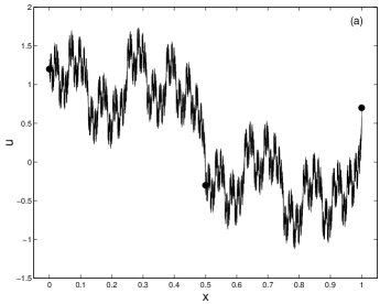
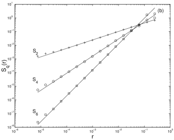
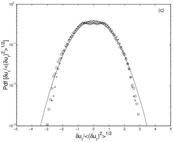
Figure 1: (a) A synthetic turbulence series of fractal dimension $D=5/3$. The black dots denote initial interpolating points. (b) Structure functions of order 2, 4 and 6 (as labeled) computed from the series in Figure 1a. The slopes $(\zeta_{q})$ corresponding to this particular realization are 0.62, 1.25 and 1.89, respectively. (c) Pdfs of the normalized increments of the series in Figure 1a. The plus signs correspond to $r=2^{-14}$, while the circles refer to a distance $r=2^{-6}$. The solid curve designates the Gaussian distribution for reference.

As an exploratory example, using the fractal interpolation IFS (Equation 1), we construct a $2^{17}$ points long synthetic fractal series, $u\left(x\right)$, with given coarse-grained points $\left({0.0,1.2}\right),\left({0.5,-0.3}\right)\mbox{ and }\left({1.0,0.7}\right)$ and the stretching parameters used in Scotti97 ; Scotti99 : $d_{1}=-2^{-1\mathord{\left/{\vphantom{13}}\right.\kern-1.2pt}3},d_{2}=2^{-1\mathord{\left/{\vphantom{13}}\right.\kern-1.2pt}3}$. Clearly, Figure 1a depicts that the synthetic series has fluctuations at all scales and it passes through all three interpolating points.

Next, from this synthetic series we compute higher-order structure functions (see Figure 1b for orders $2,4$ and $6$), where the $q^{th}$-order structure function, $S_{q}\left(r\right)$, is defined as follows:

$$S_{q}\left(r\right)=\left\langle{\left|{u\left({x+r}\right)-u\left(x\right)}\right|^{q}}\right\rangle\sim r^{\zeta_{q}}$$ (4)

where, the angular bracket denotes spatial averaging and $r$ is a separation distance that varies in an appropriate scaling region (known as the inertial range in turbulence). If the scaling exponent $\zeta_{q}$ is a nonlinear function of $q$, then following the convention of Vicsek ; Benzi ; Juneja ; Biferale ; Bohr , the field is called multiaffine, otherwise it is termed as monoaffine. In this context, we would like to mention that, Kolmogorov’s celebrated 1941 hypothesis (a.k.a K41) based on the assumption of global scale invariance in the inertial range predicts that the structure functions of order $q$ scale with an exponent $q/3$ over inertial range separations Ann ; Frisch . Deviations from $\zeta_{q}=q/3$ would suggest inertial range intermittency and invalidate the K41 hypothesis. Inertial range intermittency is still an unresolved issue, although experimental evidence for its existence is overwhelming Ann ; Anselmet . To interpret the curvilinear behavior of the $\zeta_{q}$ function observed in experimental measurements (e.g., Anselmet ), Parisi and Frisch Parisi ; Frisch proposed the multifractal model, by replacing the global scale invariance with the assumption of local scale invariance. They conjectured that at very high Reynolds number, turbulent flows have singularities (almost) everywhere and showed that the singularity spectrum is related to the structure function-based scaling exponents, $\zeta_{q}$ by the Legendre transformation.

Our numerical experiment with the stretching parameters of Scotti97 ; Scotti99 , i.e., $\left|d_{1}\right|=\left|d_{2}\right|=2^{-1\mathord{\left/{\vphantom{13}}\right.\kern-1.2pt}3}$, revealed that the scaling exponents follow the K41 predictions (after ensemble averaging over one hundred realizations corresponding to different initial interpolating points), i.e., $\zeta_{q}=q/3$ (not shown here), a signature of monoaffine fields. Later on, we will give analytical proof that indeed this is the case for $\left|{d_{1}}\right|=\left|{d_{2}}\right|=2^{-1\mathord{\left/{\vphantom{13}}\right.\kern-1.2pt}3}$. Also, in this case, the pdfs of the velocity increments, $\delta u_{r}\left(x\right)=u\left({x+r}\right)-u\left(x\right)$, always portray near-Gaussian (slightly platykurtic) behavior irrespective of $r$ (see Figure 1c). This is contrary to the observations Ann ; Anselmet , where, typically the pdfs of increments are found to be $r$ dependent and become more and more non-Gaussian as $r$ decreases. Theoretically, non-Gaussian characteristics of pdfs correspond to the presence of intermittency in the velocity increments and gradients (hence in the energy dissipation) Frisch ; Ann ; Benzi ; Bohr .

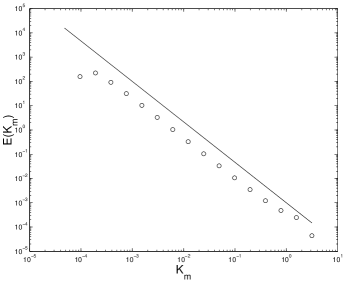
Figure 2: Wavelet power spectrum (cirlces) of the series in Figure 1a. The -5/3 power law is also shown for comparison.

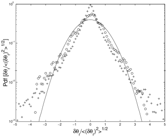
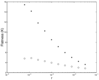
Figure 7: (a) Pdfs of the normalized increments of the passive scalar Multiaffine series. The plus signs refer to distance $r=2^{-14}$, while the circles to a distance $r=2^{-6}$. The solid curve designates the Gaussian distribution for reference. (b) The flatness factors of the pdfs of the increments of the velocity (circles) and passive-scalar field (stars) as a function of distance $r$. Note that both the fields approach the Gaussian value of 3 only at large separation distances. Clearly the passive-scalar field is more non-Gaussian than the velocity field.

In Figure 2, we plot the wavelet spectrum of this synthetic series. Due to the dyadic nature of the fractal interpolation technique, the Fourier spectrum will exhibit periodic modulation (see Figures 7 and 8 of Scotti99 ). To circumvent this issue we make use of the (dyadic) discrete Haar wavelet transform. Following Katul , the wavelet power spectral density function $E(K_{m})$ is defined as:

$$E\left({K_{m}}\right)=\frac{\left\langle{\left({WT^{\left(m\right)}\left[i\right]}\right)^{2}}\right\rangle dx}{2\pi\ln\left(2\right)}\\$$ (5)

where, wavenumber $K_{m}(=\frac{2\pi}{2^{m}dx})$ corresponds to scale $R_{m}(=2^{m}dx)$. The scale index $m$ runs from $1$ (finest scale) to $log_{2}(N)$ (coarsest scale). $WT^{\left(m\right)}\left[i\right]$, $dx$ and $N$ denote the Haar wavelet coefficient at scale $m$ and location $i$, spacing in physical space and length of the spatial series, respectively. The power spectrum displays the inertial range slope of $-5/3$, as anticipated.

At this point, we would like to invoke an interesting mathematical result regarding the scaling exponent spectrum, $\zeta_{q}$, of the fractal interpolation IFS Levy :

$$\zeta_{q}=1-\log_{N}\sum\limits_{n=1}^{N}{\left|{d_{n}}\right|^{q}}$$ (6)

where, $N$ = the number of anchor points $-1$ (in our case $N=2$). The original formulation of Levy was in terms of a more general scaling exponent spectrum, $\tau\left(q\right)$, rather than the structure function based spectrum $\zeta_{q}$. The $\tau\left(q\right)$ spectrum is an exact Legendre tranform of the singularity spectrum in the sense that it is valid for any order of moments (including negative) and any singularities Muzy ; Jaff . $\tau\left(q\right)$ can be reliably estimated from data by the Wavelet-Transform Modulus-Maxima method Muzy ; Jaff . To derive Equation 6 from the original formulation, we made use of the equality: $\tau\left(q\right)=\zeta_{q}-1$, which holds for positive $q$ and for positive singularities of Hölder exponents less than unity Muzy ; Jaff . In turbulence, the most probable Hölder exponent is 0.33 (corresponding to the K41 value) and for all practical purposes the values of Hölder exponents lie between $0$ and $1$ (see Bacry ; Verg ). Hence the use of the above equality is well justified.

Equation 6 could be used to validate our previous claim, that the parameters of Scotti97 ; Scotti99 give rise to a monoaffine field (i.e., $\zeta_{q}$ is a linear function of $q$). If we consider $\left|{d_{1}}\right|=\left|{d_{2}}\right|=d=2^{-1\mathord{\left/{\vphantom{13}}\right.\kern-1.2pt}3}$, then, $\zeta_{q}=1-\log_{2}\left({\left|{d_{1}}\right|^{q}+\left|{d_{2}}\right|^{q}}\right)=1-\log_{2}\left({2d^{q}}\right)=-q\log_{2}\left(d\right)=-q\log_{2}\left({2^{-1\mathord{\left/{\vphantom{13}}\right.\kern-1.2pt}3}}\right)=q/3$ [QED]. Equation 6 could also be used to derive the classic result of Barnsley regarding the fractal dimension of IFS. It is well-known Mando ; Davis that the graph dimension (or box-counting dimension) is related to $\zeta_{1}$ as follows: $D=2-\zeta_{1}.$ Now, using Equation 6 we get, $D=2-\zeta_{1}=1+\log_{N}\sum\limits_{n=1}^{N}{\left|{d_{n}}\right|}$. For $N=2$, we recover Equation 3.

Intuitively, by prescribing several scaling exponents, $\zeta_{q}$ (which are known apriori from observational data), it is possible to solve for $d_{n}$ from the overdetermined system of equations (Equation 6). These solved parameters, $d_{n}$, along with other easily derivable (from the given anchor points and $d_{n}$) parameters ($a_{n},c_{n},e_{n}$ and $f_{n}$) in turn can be used to construct multiaffine signals. For example, solving for the values quoted by Frisch Frisch : $\zeta_{2}=0.70,\zeta_{3}=1,\zeta_{4}=1.28,\zeta_{5}=1.53,\zeta_{6}=1.77,\zeta_{7}=2.01$ and $\zeta_{8}=2.23$, along with $\zeta_{1}=0.33$ (corresponding to $D=5/3$), yields the stretching factors $\left|d_{n}\right|=0.887,0.676$. There are altogether eight possible sign combinations for the above stretching parameter magnitudes and all of them can potentially produce multiaffine fields with the aforementioned scaling exponents. However, all of them might not be the “right” candidate from the LES-performance perspective. Rigorous a-priori and a-posteriori testing of these Multiaffine SGS models is needed to elucidate this issue (see Section V).

We repeated our previous numerical experiment with the stretching parameters $d_{1}=-0.887$ and $d_{2}=0.676$. Figure 3a shows the measured values (ensemble averaged over one hundred realizations) of the scaling exponents $\zeta_{q}$ upto $12^{th}$ order. For comparison we have also shown the theoretical values computed directly from Equation 6 (dashed line). A model proposed by She and Lévêque She based on a hierarchy of fluctuation structures associated with the vortex filaments is also shown for comparison (dotted line). We chose this particular model because of its remarkable agreement with experimental data. The She and Lévêque model predicts: $\zeta_{q}=\frac{q}{9}+2-2(\frac{2}{3})^{q\mathord{\left/{\vphantom{13}}\right.\kern-1.2pt}3}$. Figure 3b shows the pdfs of the increments, which are quite similar to what is observed in real turbulence – for large $r$ the pdf is near Gaussian while for smaller $r$ it becomes more and more peaked at the core with high tails (see also Figure 7b for the variation of flatness factors of the pdfs of increments with distance $r$).

IV Fractal Calculus and Subgrid-Scale Modeling

In the case of an incompressible fluid, the spatially filtered Navier-Stokes equations are:

$$\frac{\partial\tilde{u}_{m}}{\partial x_{m}}=0,$$ (7a)

$$\frac{\partial\tilde{u}_{m}}{\partial t}+\tilde{u}_{n}\frac{\partial\tilde{u}_{m}}{\partial x_{n}}=-\frac{\partial}{\partial x_{n}}\left[{\frac{\tilde{p}}{\rho}\delta_{mn}+\tau_{mn}}\right]+\nu\nabla^{2}\tilde{u}_{m}$$ (7b)

$$\mbox{}m,n=1,2,3.$$

where $t$ is time, $x_{n}$ is the spatial coordinate in the $n$-direction, $u_{n}$ is the velocity component in the $n$-direction, $p$ is the dynamic pressure, $\rho$ is the density and $\nu$ is the molecular viscosity of the fluid. The tilde $\tilde{(\hskip 7.22743pt)}$ denotes the filtering operation, using a filter of characteristic width $\Delta$ Footnote1 . These filtered equations are now amenable to numerical solution (LES) on a grid with mesh-size of order $\Delta$, considerably larger than the smallest scale of motion (the Kolmogorov scale). However, the SGS stress tensor $\tau_{mn}$ in Equation 7b, defined as

$$\tau_{mn}=\widetilde{u_{m}u_{n}}-\tilde{u}_{m}\tilde{u}_{n}\\$$ (8)

is not known. It essentially represents the contribution of unresolved scales (smaller than $\Delta$) to the total momentum transport and must be parameterized (via a SGS model) as a function of the resolved velocity field. Due to strong influence of the SGS parameterizations on the dynamics of the resolved turbulence, considerable research efforts have been made during the past decades and several SGS models have been proposed (see Meneveau-Katz ; Sagaut for reviews). The Eddy-viscosity model (Smagorinsky ) and its variants (e.g., the Dynamic model Germano , the Scale-Dependent Dynamic model Porte1 ) are perhaps the most widely used SGS models. They parameterize the SGS stresses as being proportional to the resolved velocity gradients. These SGS models and other standard models (e.g., Similarity, Nonlinear, Mixed models) postulate the form of the SGS stress tensors rather than the structure of the SGS fields (Mazzino ). Philosophically a very different approach would be to explicitly reconstruct the subgrid-scales from given resolved scale values (by exploiting the statistical structures of the unresolved turbulent fields) using a specific mathematical tool (e.g., the Fractal Interpolation Technique) and subsequently estimate the relevant SGS tensors necessary for LES. The Fractal model of Scotti97 ; Scotti99 and our proposed Multiaffine model basically represent this new class of SGS modeling, also known as the “direct modeling of SGS turbulence” (Meneveau-Katz ; Sagaut ; Doma ).

In Section III, we have demonstrated that FIT could be effectively used to generate synthetic turbulence fields with desirable statistical properties. In addition, Barnsley’s rigorous fractal calculus offers the ability to analytically evaluate any statistical moment of these synthetically generated fields, which in turn could be used for SGS modeling. Detailed discussion of the fractal calculus is beyond the scope of this paper. Below, we briefly summarize the equations most relevant to the present work. Let us first consider the moment integral: $U_{l,m}=\int\limits_{0}^{1}{x^{m}\left[{u\left(x\right)}\right]^{l}dx}.$ In the present context $(x_{0}=0,x_{1}=0.5\mbox{ and }x_{2}=1)$, this moment integral could be viewed as $2\Delta$ filtering $(\Delta=0.5)$ with the Top Hat filter $\mbox{[ i.e., }F_{\Delta}\left({x}\right)=1/\Delta,\mbox{ if }\left|{x}\right|<\Delta/2\mbox{ and }F_{\Delta}(x)=0,\mbox{ otherwise }\mbox{]}$. For instance, the 1-D component of the SGS stress tensor reads as:

$$\tau= \widetilde{uu} -\tilde{u}\tilde{u}$$ (9a)

$$= U_{2,0} -U_{1,0}U_{1,0}$$ (9b)

Barnsley (Barn86 ) proved that for the fractal interpolation IFS (Equation 1), the moment integral becomes:

$$U_{l,m}=\frac{\left({\sum\limits_{j=0}^{m-1}{U_{l,j}}\left({{\begin{array}[]{*{20}c}m\hfill\\ j\hfill\\ \end{array}}}\right)\sum\limits_{n=1}^{2}{a_{n}^{j+1}d_{n}e_{n}^{m-j}}+\sum\limits_{p=0}^{l-1}{\sum\limits_{j=0}^{l+m-p}{K\left({l,m,p,j}\right)U_{p,j}}}}\right)}{\left({1-\sum\limits_{n=1}^{2}{a_{n}^{m+1}d_{n}^{l}}}\right)}\\$$ (10a)

where,

$$\sum\limits_{n=1}^{2}{\left({{\begin{array}[]{*{20}c}l\hfill\\ p\hfill\\ \end{array}}}\right)a_{n}\left({c_{n}x+f_{n}}\right)^{l-p}d_{n}^{p}\left({a_{n}x+e_{n}}\right)^{m}=\sum\limits_{j=0}^{l+m-p}{K\left({l,m,p,j}\right)x^{j}}}$$ (10b)

After some algebraic manipulations, the SGS stress equation at node $x_{i}$ becomes:

$$\tau_{i}= \alpha_{0}\tilde{u}_{i-1}^{2}+\alpha_{1}\tilde{u}_{i}^{2}+\alpha_{2}\tilde{u}_{i+1}^{2}+$$ (11)

$$\alpha_{3}\tilde{u}_{i-1}\tilde{u}_{i}+\alpha_{4}\tilde{u}_{i}\tilde{u}_{i+1}+\alpha_{5}\tilde{u}_{i+1}\tilde{u}_{i-1}$$

We would like to point out that the coefficients $\alpha_{k}$ are sole functions of the stretching factors $d_{n}$. In other words, if one can specify the values of $d_{n}$ in advance, the SGS stress ($\tau$) could be explicitly written in terms of the coarse-grained (resolved) velocity field ($\tilde{u}_{i}$) weighted according to weights $\alpha_{k}$ uniquely determined by $d_{n}$. In Table 1, we have listed the $\alpha_{k}$ values corresponding to eight stretching factor combinations, $\left|d_{n}\right|=0.887,0.676$. It is evident that any two combinations ($d_{1},d_{2}$) and ($d_{2},d_{1}$) are simply “mirror” images of each other in terms of $\alpha_{k}$. Thus, only four distinct Multiaffine SGS models (M1, M2, M3 and M4) could be formed from the aforementioned eight $\left|d_{n}\right|$ combinations and in each case the orderings could be chosen at random with equal probabilities. In this table, we have also included the Fractal model of Scotti97 ; Scotti99 and the Similarity model of Bard in expanded form similar to the Multiaffine models (see the Appendix for more information on standard SGS models). The Multiaffine models and the Fractal model differ slightly in terms of filtering operation. Scotti97 ; Scotti99 performed filtering at a scale $\Delta$ (see Equation 16b), whereas in the case of Similarity model, Liu found that it is more appropriate to filter at $2\Delta$. For the Multiaffine models, we also chose to employ $2\Delta$ filtering scale.

One noticable feature in Table 1 is that some combinations of $d_{n}$ result in strongly asymmetric weights $\alpha_{k}$. As an example, in the case of M4 with $d_{1}=+0.676$ and $d_{2}=+0.887$, $|\alpha_{0}|\gg|\alpha_{2}|$ and $|\alpha_{3}|\gg|\alpha_{4}|$. This means that the SGS stress at any node $x_{i}$ would have more weight from the resolved velocity at node $x_{i-1}$ than node $x_{i+1}$. One would expect that such an asymmetry could have serious implication in terms of SGS model performance.

In the following section, we will attempt to address this issue among others by evaluating several SGS models via the a-priori analysis approach.

Table 1: The Multiaffine, Fractal and Similarity SGS models in expanded form and their corresponding coefficients for the computation of SGS stresses according to Equation 11.

Model	$(d_{1},d_{2})$	Filter Width	$\alpha_{0}$	$\alpha_{1}$	$\alpha_{2}$	$\alpha_{3}$	$\alpha_{4}$	$\alpha_{5}$
Multiaffine (M1)	$(-0.887,+0.676)$	$2\Delta$	$0.218$	$0.204$	$0.050$	$-0.372$	$-0.036$	$-0.065$
	$(+0.676,-0.887)$	$2\Delta$	$0.050$	$0.204$	$0.218$	$-0.036$	$-0.372$	$-0.065$
Multiaffine (M2)	$(+0.887,-0.676)$	$2\Delta$	$0.030$	$0.248$	$0.261$	$-0.018$	$-0.479$	$-0.043$
	$(-0.676,+0.887)$	$2\Delta$	$0.261$	$0.248$	$0.030$	$-0.479$	$-0.018$	$-0.043$
Multiaffine (M3)	$(-0.887,-0.676)$	$2\Delta$	$0.144$	$0.220$	$0.133$	$-0.230$	$-0.209$	$-0.057$
	$(-0.676,-0.887)$	$2\Delta$	$0.133$	$0.220$	$0.144$	$-0.209$	$-0.230$	$-0.057$
Multiaffine (M4)	$(+0.887,+0.676)$	$2\Delta$	$0.064$	$0.319$	$0.262$	$-0.121$	$-0.517$	$-0.007$
	$(+0.676,+0.887)$	$2\Delta$	$0.262$	$0.319$	$0.064$	$-0.517$	$-0.121$	$-0.007$
Fractal	$(-0.794,+0.794)$	$\Delta$	$0.127$	$0.221$	$0.026$	$-0.322$	$-0.120$	$+0.069$
	$(+0.794,-0.794)$	$\Delta$	$0.026$	$0.221$	$0.127$	$-0.120$	$-0.322$	$+0.069$
Similarity	NA	$2\Delta$	$0.188$	$0.250$	$0.188$	$-0.250$	$-0.250$	$-0.125$

V Evaluation of SGS Models: A-priori Analysis Approach

The SGS models and their underlying hypotheses can be evaluated by two approaches: a-priori testing and a-posteriori testing (terms coined by Piomelli ). In a-posteriori testing, LES computations are actually performed with proposed SGS models and validated against reference solutions (in terms of mean velocity, scalar and stress distributions, spectra etc.). However, owing to the multitude of factors involved in any numerical simulation (e.g., numerical discretizations, time integrations, averaging and filtering), a-posteriori tests in general do not provide much insight about the detailed physics of the newly implemented SGS models Meneveau-Katz ; Sagaut . A complementary and perhaps more fundamental approach Meneveau-Katz would be to use high-resolution model (Direct Numerical Simulation or DNS), experimental or field observational data to compute the “real” and modeled SGS tensors directly from their definitions and compare them subsequently. This approach, widely known as the a-priori analysis, does not require any actual LES modeling and is theoretically more tractable. In this work we focused on comparing the performance of SGS models via the a-priori analysis. We strictly followed the 1-D apriori analysis approach of Meneveau ; Oneil ; Porte2 . To highlight the caveats of the proposed and several existing SGS models, we performed an extensive inter-model comparison study. This exercise also helped selecting the “right” combination of stretching factors for the Multiaffine SGS models.

In general, the correlation between real ($\tau^{Real}$) and modeled ($\tau^{Model}$) SGS stresses is considered to be a good indicator of the expected performance of a proposed SGS model. Another crucial indicator is the so called SGS energy dissipation rate ($\Pi$):

$$\Pi = -\tau_{ij}\tilde{S}_{ij}$$

$$\approx -\frac{15}{2}\tau\frac{\partial\tilde{u}}{\partial x}\mbox{~{}(1-D approximation)}$$

In the inertial range, the SGS energy dissipation rate is the most influential factor affecting the dynamical evolution of the resolved kinetic energy Meneveau-Katz . On average, $\Pi$ is positive, representing a net drain of resolved kinetic energy into unresolved motion. Intermittent negative values of $\Pi$, known as “backscatter”, implies energy transfer from SGS to resolved scales. Unfortunately, a high correlation between real and modeled SGS stress (or SGS energy dissipation rate) is not a sufficient condition for the success of a proposed LES SGS model, although it is a highly desirable feature Liu ; Meneveau ; Sagaut .

We primarily made use of an extensive atmospheric boundary layer (ABL) turbulence dataset (comprising of fast-response sonic anemometer data) collected by various researchers from the Johns Hopkins University, the University of California-Davis and the University of Iowa during Davis 1994, 1995, 1996, 1999 and Iowa 1998 field studies. Comprehensive description of these field experiments (e.g., surface cover, fetch, instrumentation, sampling frequency) can be found in Pahlow . We further augmented this dataset with nocturnal ABL turbulence data from CASES-99 (Cooperative Atmosphere-Surface Exchange Study 1999), a cooperative field campaign conducted near Leon, Kansas during October 1999 Poulos . For our analyses four levels (1.5, 5, 10 and 20m) of sonic anemometer data from the 60m tower and the adjacent mini-tower collected during two intensive observational periods (nights of October $17^{th}$ and $19^{th}$) were considered [the sonic anemometer at 1.5m was moved to 0.5m level on October $19^{th}$]. Briefly, the collective attributes of the field dataset explored in this study are as follows: (i) surface cover: bare soil, grass and beans; (ii) sampling frequency: 18 to 60 Hz; (iii) sampling period: 20 to 30 minutes; (iv) sensor height ($z$): 0.5 to 20m; and (v) atmospheric stability ($z/L$, $L$ is the local Obukhov length):  0 (neutral) to  10 (very stable).

ABL field measurements are seldom free from mesoscale disturbances, wave activities, nonstationarities etc. The situation could be further aggravated by several kinds of sensor errors (e.g., random spikes, amplitude resolution error, drop outs, discontinuities etc.). Thus, stringent quality control and preprocessing of field data is of utmost importance for any rigorous statistical analysis. Our quality control and preprocessing strategies are qualitatively similar to the suggestions of Mahrt1 . Specifically, we follow these steps:

(1) Visual inspection of individual data series for detection of spikes, amplitude resolution error, drop outs and discontinuities. Discard suspected data series from further analyses.

(2) Adjust for changes in wind direction by aligning sonic anemometer data using 60 seconds local averages of the longitudinal and transverse component of velocity.

(3) Partitioning of turbulent-mesoscale motion using discrete wavelet transform (Symmlet-8 wavelet) with a gap scale Mahrt2 of 100 seconds.

(4) Finally, to check for nonstationarities of the partitioned series, we performed the following step: we subdivided each series in 6 equal intervals and computed the standard deviation of each sub-series ($\sigma_{i},~{}i=1:6$). If $max(\sigma_{i})/min(\sigma_{i})>2$, the series was discarded.

After all these quality control and preprocessing steps, we were left with only 358 “reliable” series for a-priori analyses. These streamwise velocity series were filtered with a Top-Hat filter ($\Delta=$ 1,2,4 or 8m) and downsampled on the scale of the LES grid ($\Delta$) to obtain the resolved velocity field $\tilde{u}_{i}$ Footnote2 . In a similar way, the streamwise SGS stress, $\tau^{Real}$, was computed from its definition (Equation 9a). Filtering operations were always performed in time and interpreted as 1-D spatial filtering in the streamwise direction by means of Taylor’s frozen flow hypothesis. The spatial derivatives were also computed from the time derivatives by invoking Taylor’s hypothesis: $\frac{\partial}{\partial x}=-{\frac{1}{<u>}}{\frac{\partial}{\partial t}}$, where, $<u>$ is the mean streamwise velocity.

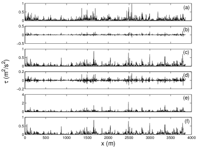
Figure 4: A comparison of the real and modeled SGS stresses, computed from atmospheric boundary layer measurements, using 1-D filtering and Taylor’s hypothesis. The filter width $\Delta$ is 2m. (a) Real, (b) Smagorinsky model, (c) Similarity model, (d) SGS kinetic energy based model, (e) Fractal model, and (f) Multiaffine model (M3).

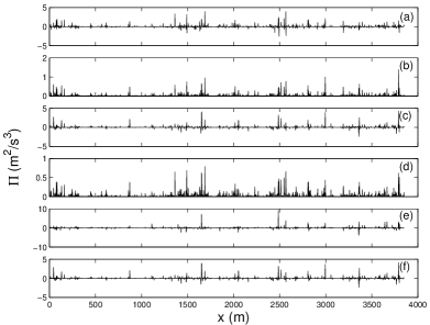
Figure 5: A comparison of the real and modeled SGS energy dissipation rates, computed from atmospheric boundary layer measurements, using 1-D filtering and Taylor’s hypothesis. The filter width $\Delta$ is 2m. (a) Real, (b) Smagorinsky model, (c) Similarity model, (d) SGS kinetic energy based model, (e) Fractal model, and (f) Multiaffine model (M3).

In Figure 4 representative realizations of the real and several modeled SGS stresses are presented. The modeled SGS stresses, $\tau^{Model}$ were computed from the definitions given in the Appendix. Along the same lines, the real and modeled SGS energy dissipation rates (Figure 5) were calculated according to $\Pi^{Real}=-\frac{15}{2}\tau^{Real}\frac{\partial\tilde{u}}{\partial x}$ and $\Pi^{Model}=-\frac{15}{2}\tau^{Model}\frac{\partial\tilde{u}}{\partial x}$, respectively. The SGS model constants like $C_{S}$ of the Smagorinsky model or $C_{L}$ of the Similarity model (see Appendix) were obtained by matching the mean real and modeled SGS energy dissipation rates Meneveau ; Oneil ; Porte2 . For consistency, the same procedure was followed for the SGS-kinetic-energy-based model, Fractal model and Multiaffine models. In other words, we always ensured that $<-\frac{15}{2}\tau^{Real}\frac{\partial\tilde{u}}{\partial x}>~{}=~{}<-\frac{15}{2}\tau^{Model}\frac{\partial\tilde{u}}{\partial x}>$. Note that, this procedure has no effect on the correlation results presented below. In actual simulations these model coefficients could be obtained dynamically following the approach of Germano ; Lilly .

From Figures 4 and 5 it is visually evident that both Similarity and Multiaffine models capture the variability of the SGS stress and energy dissipation rates reasonably well. On the other hand, the performances of the Smagorinsky and SGS-kinetic-energy-based models are very poor. Note that, the Smagorinsky model assumes that the trace of the SGS tensor is subtracted from the tensor, which is not feasible in 1-D a-priori analysis Meneveau . Thus, direct magnitude-wise comparison between real and the Smagorinsky model based SGS stress or dissipation energy is not possible. However, this does not prevent us from quantifying the performance by correlation coefficient. Moreover, the Smagorinsky model is by construction fully dissipative. Hence, this model is unable to reproduce the backscatter effects (see Figure 5b), which do occur in the real SGS dissipation series (Figure 5a).

In Table 2, for $\Delta=$ 1m, we show the correlation between the real and modeled SGS stress and energy dissipation rates. The standard deviations are given in parentheses. The model M3 is significantly better than any other Multiaffine model and this could only be attributed to its near-symmetric stencil structure (see Table 1). This resolves our previous dilemma regarding the selection of one Multiaffine SGS model from a class of four. From here on, we’ll only report results for M3 and will identify it as the Multiaffine model.

Table 2: Average correlation between observed and modeled SGS stresses and energy dissipation rates $(\Delta=1$m). The results are based on 358 ABL turbulent velocity series measured during several field campaigns. The quantities in the parenthesis represent standard deviation.

	Corr$(\tau^{Real},\tau^{Model})$	Corr$(\Pi^{Real},\Pi^{Model})$
Smagorinsky	$0.25(0.09)$	$0.41(0.17)$
Similarity	$0.49(0.10)$	$0.76(0.15)$
SGS-KE	$0.23(0.08)$	$0.42(0.17)$
Fractal	$0.33(0.05)$	$0.61(0.06)$
Multiaffine (M1)	$0.44(0.05)$	$0.71(0.05)$
Multiaffine (M2)	$0.40(0.05)$	$0.68(0.06)$
Multiaffine (M3)	$0.49(0.05)$	$0.77(0.05)$
Multiaffine (M4)	$0.42(0.05)$	$0.70(0.05)$

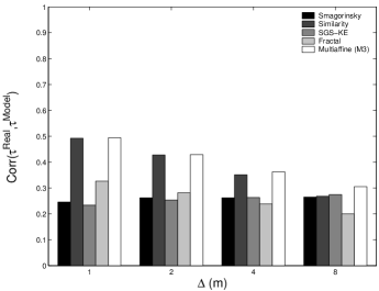
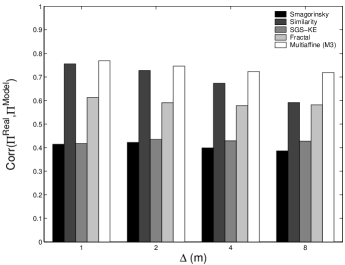
Figure 6: (a) Correlation between observed and modeled subgrid-scale stresses and (b) correlation between observed and modeled subgrid-scale energy dissipations as a function of filter width $\Delta$. The results are based on 358 ABL turbulent velocity series measured during several field campaigns.

Next, in Figure 6, we plot the mean correlation between real and modeled SGS stress and energy dissipation rates for $\Delta$ = 1,2,4 and 8m. As anticipated, for all the models, the correlation decreases with increasing filtering scale. Also, the correlation of real vs. model SGS energy dissipation rates is usually higher compared to the SGS stress scenario, as noticed by other researchers.

It is expected that in the ABL the scaling exponent values ($\zeta_{q}$) would deviate from the values reported in Frisch due to near-wall effect. This means that the stretching factors $d_{n}$ based on the $\zeta_{q}$ values we used in this work, are possibly in error. Nevertheless, the overall performance of the Multiaffine model is beyond our expectations. It remains to be seen how the proposed SGS scheme will perform in a-posteriori analysis and such work is currently in progress.

VI Passive Scalar

Our scheme could be easily extended to synthetic passive-scalar (any diffusive component in a fluid flow that has no dynamical effect on the fluid motion itself, e.g., a pollutant in air, temperature in a weakly heated flow, a dye mixed in a turbulent jet or moisture mixing in air War ; Sigg ) field generation. The statistical and dynamical characteristics (anisotropy, intermittency, pdfs etc.) of passive-scalars are surprisingly different from the underlying turbulent velocity field War ; Sigg . For example, it is even possible for the passive-scalar field to exhibit intermittency in a purely Gaussian velocity field War ; Sigg . Similar to the K41, neglecting intermittency, the Kolmogorov-Obukhov-Corrsin (KOC) hypothesis predicts that at high Reynolds and Peclet numbers, the $q^{th}$-order passive-scalar structure function will behave as: $\left\langle{\left|{\theta\left({x+r}\right)-\theta\left(x\right)}\right|^{q}}\right\rangle\sim r^{\frac{q}{3}}$ in the inertial range. Experimental observations reveal that analogous to turbulent velocity, passive-scalars also exhibit anomalous scaling (departure from the KOC scaling). Observational data also suggest that passive-scalar fields are much more intermittent than velocity fields and result in stronger anomaly War ; Sigg .

To generate synthetic passive-scalar fields, we need to determine the stretching parameters $d_{1}$ and $d_{2}$ from prescribed scaling exponents, $\zeta_{q}$. Unlike the velocity scaling exponents, the published values (based on experimental observations) of higher-order passive-scalar scaling exponents display significant scatter. Thus for our purpose, we used the predictions of a newly proposed passive-scalar model Feng : $\zeta_{q}=2+\left({\frac{8}{9}}\right)^{2}-2\left({\frac{3}{4}}\right)^{q\mathord{\left/{\vphantom{q6}}\right.\kern-1.2pt}6}-\left({\frac{8}{9}}\right)^{2}\left({\frac{7}{16}}\right)^{q\mathord{\left/{\vphantom{q2}}\right.\kern-1.2pt}2}$. This model based on the hierarchical structure theory of She shows reasonable agreement with the observed data. Moreover, unlike other models, this model manages to predict that the scaling exponent $\zeta_{q}$ is a nondecreasing function of $q$. Theoretically, this is crucial because, otherwise, if $\zeta_{q}\to-\infty$ as $q\to+\infty$, the passive-scalar field cannot be bounded Frisch ; Feng .

Employing Equation (6) and the scaling exponents (upto $8^{th}$-order) predicted by the above model, we get the following stretching factors: $\left|d_{n}\right|=0.964,0.606$. We again repeated the numerical experiment of section III and selected the stretching parameter combination: $d_{1}=-0.964$ and $d_{2}=0.606$. Like before, we compared the estimated [using Equation (4)] scaling exponents from one hundred realizations with the theoretical values [from Equation (6)] and the agreement was found to be highly satisfactory. To check whether a generated passive-scalar field ($d_{1}=-0.964$, $d_{2}=0.606$) possesses more non-Gaussian characteristics than its velocity counterpart ($d_{1}=-0.887$, $d_{2}=0.676$), we performed a simple numerical experiment. We generated both the velocity and passive-scalar fields from identical anchor points and also computed the corresponding flatness factors, $K$, as a function of distance $r$ (see Figure 7b). Comparing Fig 7a with Fig 3b and also from Fig 7b, one could conclude that the passive-scalar field exhibits stronger non-Gaussian behavior than the velocity field, in accord with the literature.

VII Concluding Remarks

In this paper, we propose a simple yet efficient scheme to generate synthetic turbulent velocity and passive-scalar fields. This method is competitive with most of the other synthetic turbulence emulator schemes (e.g., Vicsek ; Benzi ; Juneja ; Biferale ; Bohr ) in terms of capturing small-scale properties of turbulence and scalars (e.g., multiaffinity and non-Gaussian characteristics of the pdf of velocity and scalar increments). Moreover, extensive a-priori analyses of field measurements unveil the fact that this scheme could be effectively used as a SGS model in LES. Potentially, the proposed Multiaffine SGS model can address two of the unresolved issues in LES: it can systematically account for the near-wall and atmospheric stability effects on the SGS dynamics. Of course, this would require some kind of universal dependence of the scaling exponents on both wall-normal distance and stability. Quest for this kind of universality has began only recently Ruiz ; Aivalis .

*

Appendix A

The standard Smagorinsky eddy-viscosity model is of the form:

$$\tau^{Smag}_{ij}=-2(C_{S}\Delta)^{2}|\tilde{S}|\tilde{S}_{ij}$$ (13a)

where,

$$\tilde{S}_{ij}=\frac{1}{2}({\frac{\partial\tilde{u}_{i}}{\partial x_{j}}+\frac{\partial\tilde{u}_{j}}{\partial x_{i}}})$$

is the resolved strain rate tensor and

$$|\tilde{S}|=({2\tilde{S}_{ij}\tilde{S}_{ij}})^{1/2}$$

is the magnitude of the resolved strain rate tensor. $$C_{S}$$ is the so-called Smagorinsky coefficient.

For 1-D surrogate SGS stress:

$$\tilde{S}_{11}=\frac{\partial\tilde{u}}{\partial x}$$

Further, by assuming that the smallest scales of the resolved motion are isotropic, the following equality holds Monin :

$$<\tilde{S}_{ij}\tilde{S}_{ij}>=\frac{15}{2}<\tilde{S}_{11}^{2}>$$

Employing this assumption for the instantaneous fields, we can write

$$|\tilde{S}|=({2\tilde{S}_{ij}\tilde{S}_{ij}})^{1/2}\approx\sqrt{15}|{\frac{\partial\tilde{u}}{\partial x}}|$$

Hence, the Smagorinsky SGS stress equation becomes:

$$\tau^{Smag}=-2({C_{S}\Delta})^{2}\sqrt{15}|{\frac{\partial\tilde{u}}{\partial x}}|({\frac{\partial\tilde{u}}{\partial x}})$$ (13b)

The second model we considered is the Similarity Model Bard ; Liu .

$$\tau^{Siml}_{ij}=C_{L}(\overline{\tilde{u}_{i}\tilde{u}_{j}}-{\overline{\tilde{u}}}_{i}~{}{\overline{\tilde{u}}}_{j})\\$$ (14a)

The overbar denotes explicit filtering with a filter of width $$\gamma\Delta \gamma=2 C_{L}$$ (usually ). is the Similarity model coefficient.

The 1-D surrogate SGS stress could be simply written as:

$$\tau^{Siml}=C_{L}(\overline{\tilde{u}\tilde{u}}-{\overline{\tilde{u}}}~{}{\overline{\tilde{u}}})\\$$ (14b)

Now, for 2$\Delta$ filtering this equation becomes:

$$\tau^{Siml}=C_{L}[({\frac{\tilde{u}_{i-1}^{2}+2\tilde{u}_{i}^{2}+\tilde{u}_{i+1}^{2}}{4}})\\ -({\frac{\tilde{u}_{i-1}+2\tilde{u}_{i}+\tilde{u}_{i+1}}{4}})^{2}]$$ (14c)

which on further simplification leads to the expression in Table 1:

$$\tau^{Siml}=C_{L}[0.188\tilde{u}_{i-1}^{2}+0.25\tilde{u}_{i}^{2}+0.188\tilde{u}_{i+1}^{2}$$

$$-0.25\tilde{u}_{i-1}\tilde{u}_{i}-0.25\tilde{u}_{i}\tilde{u}_{i+1}-0.125\tilde{u}_{i+1}\tilde{u}_{i-1}]$$

Next, we consider a SGS model based on the SGS kinetic energy $(q^{2})$ Meneveau ; Wong :

$$\tau^{Stke}=-2C_{K}^{2}\Delta\sqrt{|\tilde{q^{2}}|}{\frac{\partial\tilde{u}}{\partial x}}$$ (15a)

$$\mbox{where,~{}}q^{2}=3(u-\tilde{u})^{2}$$

Here, $C_{K}$ is the SGS model coefficient.

In the case of the Fractal model of Scotti97 ; Scotti99 , the unknown subgrid stress ($\tau$) produced by synthetic fractal field around any grid point $x_{i}$ can be written as:

$$\tau_{i}^{Frac} = \int\limits_{\frac{1}{4}}^{\frac{3}{4}}[u(x)]^{2}dx-[\int\limits_{\frac{1}{4}}^{\frac{3}{4}}u(x)dx]^{2}$$ (16b)

$$= \frac{1}{12}(\delta_{i}\tilde{u})^{2}+\frac{d_{i}(8-3d_{i}^{2})}{48}\delta_{i}^{2}\tilde{u}\delta_{i}\tilde{u}+$$

$$\frac{1+15d_{i}^{2}-24d_{i}^{4}+12d_{i}^{6}}{192(1-d_{i}^{2})}(\delta_{i}^{2}\tilde{u})^{2}.$$

where, $\delta_{i}\tilde{u}=(\tilde{u}_{i+1}-\tilde{u}_{i-1})/2,~{}\delta_{i}^{2}\tilde{u}=\tilde{u}_{i+1}-2\tilde{u}_{i}+\tilde{u}_{i-1},$ and $d_{i}=\pm 2^{-1/3}$.

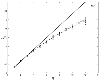
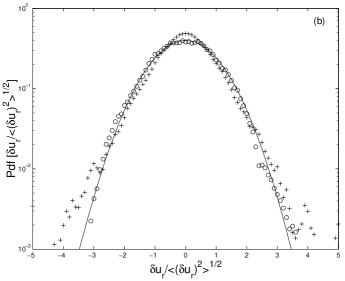
Figure 3: (a) The scaling exponent function $\zeta_{q}$. The continuous, dashed and dotted lines denote the K41, Equation 6, and the She-Lévêque model predictions respectively. The circles with error bars (one standard deviation) are estimated values over one hundred realizations using $d_{1}=-0.887$ and $d_{2}=0.676$. Experimental data of Anselmet et al.’s [5] is also shown for reference (star signs). (b) Pdfs of the normalized increments of the multiaffine series. The plus signs denote $r=2^{-14}$, while the circles refer to a distance $r=2^{-6}$. The solid curve designates the Gaussian distribution for reference.

References

- (1) T. Vicsek and A. L. Barabási, J. Phys. A 24, L845 (1991).
- (2) R. Benzi, L. Biferale, A. Crisanti, G. Paladin, M. Vergassola, and A. Vulpiani, Physica D 65, 352 (1993).
- (3) A. Juneja, D. P. Lathrop, K. R. Sreenivasan, and G. Stolovitzky, Phys. Rev. E 49, 5179 (1994).
- (4) L. Biferale, G. Boffetta, A. Celani, A. Crisanti, and A. Vulpiani, Phys. Rev. E 57, R6261 (1998).
- (5) T. Bohr, M. H. Jensen, G. Paladin, and A. Vulpiani, Dynamical Systems Approach to Turbulence, (Cambridge University Press, Cambridge, UK, 1998).
- (6) A. Scotti and C. Meneveau, Phys. Rev. Lett. 78, 867 (1997).
- (7) A. Scotti and C. Meneveau, Physica D 127, 198 (1999).
- (8) M. F. Barnsley, Constr. Approx. 2, 303 (1986).
- (9) M. F. Barnsley, Fractals Everywhere, (Academic Press, Boston, MA, 1993).
- (10) A. Scotti, C. Meneveau, and S. G. Saddoughi, Phys. Rev. E. 51, 5594 (1995).
- (11) K. R. Sreenivasan and R. A. Antonia, Ann. Rev. Fluid Mech. 29, 435 (1997).
- (12) U. Frisch, Turbulence: The Legacy of A. N. Kolmogorov, (Cambridge University Press, Cambridge, UK, 1995).
- (13) F. Anselmet, Y. Gagne, E. J. Hopfinger, and R. A. Antonia, J. Fluid Mech. 140, 63 (1984).
- (14) G. Parisi and U. Frisch, in Proceedings of the International School on Turbulence and Predictability in Geophysical Fluid Dynamics and Climate Dynamics, M. Ghil, R. Benzi, and G. Parisi (North-Holland, Amsterdam, 1985).
- (15) G. G. Katul, J. D. Albertson, C. R. Chu, and M. B. Parlange, in Wavelets in Geophysics, E. Foufoula-Georgiou, and P. Kumar (Academic Press, San Diego, 1994).
- (16) J. Lévy-Véhel, K. Daoudi, and E. Lutton, Fractals 2, 1 (1994).
- (17) J. F. Muzy, E. Bacry, and A. Arneodo, Phys. Rev. E. 47, 875 (1993).
- (18) S. Jaffard, SIAM J. Math. Anal. 28, 944 (1997).
- (19) E. Bacry, A. Arneodo, U. Frisch, Y. Gagne, and E. Hopfinger, in Turbulence and Coherent Structures, O. Métais and M. Lesieur (Kluwer, 1990).
- (20) M. Vergassola, R. Benzi, L. Biferale, and D. Pisarenko, J. Phys. A. 26, 6093 (1993).
- (21) B. Mandelbrot, Fractals: Form, Chance, and Dimension, (W. H. Freeman, New York, NY, 1977).
- (22) A. Davis, A. Marshak, W. Wiscombe, and R. Cahalan, J. Geophys. Res. 99, 8055 (1994).
- (23) Z. S. She and E. L. Lévêque Phys. Rev. Lett. 72, 336 (1994).
- (24) In most of today’s LES computations, the filtering operation is basically implicit. This means that the process of numerical discretization (of grid size ) in itself creates the filtering effect. Although explicit filtering of the grid-resolved velocity field is desirable from a theoretical point of view, limited computational resources make it impractical Eyink . However, in a-priori studies of DNS, experimental or field observations, where fine resolution velocity fields are readily available, the explicit filtering (typically with a Top Hat, Gaussian or Cutoff filter) followed by downsampling are usually performed to compute the resolved (and filtered) velocity . This issue of filtering of velocity fields should not be confused with the explicit filterings done in the cases of Similarity, Dynamic, Fractal or Multiaffine models to compute the SGS stresses or other necessary SGS tensors.
- (25) G. L. Eyink, arXiv:chao-dyn/9602019 v1, (1996).
- (26) C. Meneveau and J. Katz Ann. Rev. Fluid Mech. 32, 1 (2000).
- (27) P. Sagaut, Large Eddy Simulation for Incompressible Flows, (Springer-Verlag, Berlin, Germany, 2001).
- (28) J. Smagorinsky Mon. Wea. Rev. 91, 99 (1963).
- (29) M. Germano, U. Piomelli, P. Moin, and W. Cabot, Phys. Fluids A 3, 1760 (1991).
- (30) F. Porté-Agel, C. Meneveau, and M. B. Parlange, J. Fluid Mech. 415, 216 (2000).
- (31) M. Antonelli, A. Mazzino, and U. Rizza, J. Atmos. Sci. 60, 215 (2003).
- (32) J. A. Domaradzki and N. A. Adams, J. Turbulence 3, 1 (2002).
- (33) J. Bardina, J.H. Ferziger, and W.C. Reynolds, Am. Inst. Aeronaut. Astronaut. Pap. 80-1357 (1980).
- (34) S. Liu, C. Meneveau, and J. Katz, J. Fluid Mech. 275, 83 (1994).
- (35) U. Piomelli, P. Moin, and J. H. Ferziger, Phys. Fluids 31, 1884 (1988).
- (36) C. Meneveau, Phys. Fluids 6, 815 (1994).
- (37) J. O’Neil and C. Meneveau, J. Fluid Mech. 349, 253 (1997).
- (38) F. Porté-Agel, C. Meneveau, and M. B. Parlange, Boundary-Layer Meteorol. 88, 425 (1998).
- (39) M. Pahlow, M. B. Parlange, and F. Porté-Agel, Boundary-Layer Meteorol. 99, 225 (2001).
- (40) G. S. Poulos and Coauthors, Bull. Amer. Meteorol. Soc. 83, 555 (2002).
- (41) D. Vickers and L. Mahrt, J. Atmos. Ocean. Technol. 14, 512 (1997).
- (42) D. Vickers and L. Mahrt, J. Atmos. Ocean. Technol. 20, 660 (2003).
- (43) Following, Liu , this filtering followed by downsampling methodology is known in the literature as “consistent” a-priori analysis.
- (44) D. K. Lilly, Phys. Fluids A 4, 633 (1992).
- (45) Z. Warhaft, Ann. Rev. Fluid Mech. 32, 203 (2000).
- (46) B. I. Shraiman and E. D. Siggia, Nature 405, 639 (2000).
- (47) Q. Z. Feng, Phys. Fluids 14, 2019 (2002).
- (48) G. Ruiz-Chavarria, S. Ciliberto, C. Baudet, and E. Lévêque, Physica D 141, 183 (2000).
- (49) K. G. Aivalis, K. R. Sreenivasan, Y. Tsuji, J. C. Klewicki, and C. A. Biltoft, Phys. Fluids 14, 2439 (2002).
- (50) A. Monin and A. Yaglom, Statistical Fluid Mechanics, (MIT Press, Cambridge, MA, 1971).
- (51) V. C. Wong, Phys. Fluids A 4, 1081 (1992).