Misconceptions regarding the cancellation of self-forces in the transverse equation of motion for an electron in a bunch

Abstract

As a consequence of motions driven by external forces, self-fields originate within an electron bunch, which are different from the static case. In the case of magnetic external forces acting on an ultrarelativistic beam, the longitudinal self-interactions are responsible for CSR (Coherent Synchrotron Radiation)-related phenomena, which have been studied extensively. On the other hand, transverse self-interactions are present too. At the time being, several existing theoretical analysis of transverse dynamics rely on the so-called cancellation effect, which has been around for more than ten years. In this paper we explain why in our view such an effect is not of practical nor of theoretical importance.

DEUTSCHES ELEKTRONEN-SYNCHROTRON

DESY 03-165

October 2003

1 Introduction

Electron bunches with, among other characteristics, very small transverse emittance and high peak current are needed for the operation of XFELs [1, 2]. The bunch length for XFEL applications is of the order of 100 femtoseconds. This is achieved using a two-step strategy: first generate beams with small transverse emittance by means of a RF photocathode and, second, apply longitudinal compression at high energy using a magnetic compressor. Self-interactions may spoil the bunch characteristics, so that, in the last few years, simulation codes have been developed in order to solve the self-consistent problem of an electron bunch moving under the action of external magnetic fields and its own self-fields. These codes show that, in the case under examination, the bunching process can be treated in the zeroth order approximation by the single-particle dynamical theory: in fact we cannot neglect the CSR-induced energy spread and other wake-fields when we calculate the transverse emittance, but we can neglect them when it comes to the characterization of the longitudinal current distribution because their contribution to the longitudinal dynamics, in the high-$\gamma$ limit, is small. As actual calculations are left to simulations, the understanding of the physics of self-interactions is left to analytical studies, which are usually based on a perturbative approach: the particles move, in the zeroth order, under the influence of external guiding fields and the zeroth order motion is used to calculate the first order perturbation to the trajectory due to the self-interactions. Of course, the perturbative approach will, in the most general case, give different answers with respect to the self-consistent approach as self-interaction effects get more and more important. Nevertheless the method behind the two approaches is the same: the only difference is due to the fact that the computational power is enough to break the particle trajectories in sufficiently small parts so that the first order perturbation theory gives a satisfactory description of the bunch evolution within a given trajectory-slice. Moreover it should be noted that perturbation techniques are important from a practical viewpoint too. In fact, when it comes to facility design, one has to find a range of parameters such that the emittance dilution is small, i.e. that the self-consistent approach can be effectively substituted, from a practical viewpoint, by the perturbative one. Partial analytical studies have been performed, in the last twenty years, on transverse self-fields, and a particular effect, called cancellation, has become on fashion in the last few years [3, 4, 5, 6]. Analytical results obtained in those papers led part of the community to believe that such an effect is very fundamental and of great practical importance. We disagree with this viewpoint. In this paper we explain our reasons. In Section 2 we trace a short, conceptual history of the cancellation effect. Then we move to the description of the current state of the theory of this effect in Section 3. After this, in Section 4, we explain our arguments against the fact that the cancellation effect is of any practical and theoretical interest. Finally, in Section 5, we come to conclusions.

2 Twenty years of history

The history of the so called cancellation effect is a long-dated one. A short summing up can be of interest here since on the one hand it gives the reader a more thorough overview of the issue, while on the other it constitutes a self-contained example of how scientific progress works in time, by trial and error and, sometimes, misconception and misunderstanding.

The story begins about twenty years ago with [7]. In that pioneering work the transverse self-force, i.e. the Lorentz self-force in the transverse direction lying on the orbital plane, is calculated for a test particle in front of a beam of zero transverse extent moving in a circle , showing a singular result for $\theta_{\mathrm{min}}=(s_{\mathrm{min}}/R)\rightarrow 0$, $s_{\mathrm{min}}$ being the minimal arc length from the nearest retarded source point to the test particle and $R$ being the radius of the circle (see Eq. (8) in [7]). The singularity has a logarithmic character arising from the particular model selected, ”is due to ’nearby’ charges and is removed as the beam is given a transverse size” (quoted from [7]). This force constituted, in the late 80s, a reason for serious concern for the beam dynamics in electron storage rings. In Eq. (42) of [8], a particle off axis of a quantity $x$ with respect to the design orbit feels a total centrifugal Lorentz force with logarithmic dependence on $x$ from an ”unshielded ring of charge of vanishing height and thickness” (cited from [8], i.e. the same beam with zero transverse extent analyzed in [7]) :

$$F={2\lambda\over{R}}\left[\ln\left({{x\over{8R}}}\right)+1\right]+O(x/R)~{},$$ (3)

$\lambda$ being the constant bunch linear density.

It should be underlined that the logarithmic singularity in $x$ comes from the choice of a particular density distribution. Not all distribution choices give singular behavior as $x\rightarrow 0$. For example, in [7], a singularity is first found as $s_{\mathrm{min}}\rightarrow 0$; we found a similar result in [9]. This is also linked to the particular choice of the distribution, that is a line bunch. The singularity for $s_{\mathrm{min}}\rightarrow 0$ has actually the same reason to be as the one for $x\rightarrow 0$ when an horizontally off-axis particle is considered. Simply, if we start from a line bunch case, and we consider a test particle with $x=0$, then the singular character of the field comes into play when $s_{\mathrm{min}}\rightarrow 0$; when $x\neq 0$, one is allowed to put $s_{\mathrm{min}}=0$ and then a singularity is present in the limit for $x\rightarrow 0$. However, this is due to the choice of the density distribution and nothing else. There are many choices (for example a gaussian 2D or 3D bunch) which do not give singular fields. As a matter of fact, macroparticle simulations are based on these kind of simplified distributions, because they avoid the problem of singularities. From a practical viewpoint then, when dealing with computational problem, one should remind that macroparticle simulation do not have to cope necessarily with singularities, which arise only in the case of particular particle distribution choices: this fact should be kept in mind throughout the reading of this paper.

As we read in [8], the transverse force was ”the subject of serious concern for its effect on dynamics in electron storage ring”, in that it spoils the cancellation between the electric field term and the magnetic field, which one usually has in pure space-charge problems for the ultrarelativistic regime: the gradient of $F$ in the radial direction is, in fact, singular as $\partial F/\partial r\sim\lambda/x$ . In the same paper, it is pointed out that this force is cancelled for long beams undergoing a circular motion. In fact ”a particle undergoing betatron oscillations has simultaneous oscillation of its kinetic energy […] in curved geometry the kinetic-energy oscillation results in a first-order dynamical term in the horizontal equation of motion, which shifts the betatron frequency. For a highly relativistic beam this additional term nearly cancels a term proportional to the gradient of the CFSC” (quoted from [8]), where the CFSC, here, is just the Lorentz force: ”we define the CSFC with an overall minus sign to agree with the conventions of other authors: $F=-(E_{r}+B_{z})_{b}$” (quoted from [8]), $r$ and $z$ referring to a cylindrical coordinate system $(r,\theta,z)$ and the subscript $b$ indicating ”beam-induced components of fields”.

3 The ”cancellation effect” today

With the development of SASE FEL technology and the need of magnetic chicanes for bunch compression, the scientific community began to analyze this kind of effects in the case of short beams moving in finite arc of circles as in the bends of magnetic chicanes. The aim was to end up with a generalization of the results in [8] which was valid under more generic assumptions: not only for coasting beams in storage rings, but also for bunched beams in generic magnetic systems. A first step in that direction was claimed in [3] and in [5], to end up with a final formulation [6].

Let us briefly describe the arguments in [3]. We track the electron bunch in cylindrical coordinates with respect to the center of a designed circular orbit of radius $R$ as in [3] or [4]: $\vec{r}=r\vec{e}_{r}+r\theta\vec{e}_{s}$. Following the Hamilton-Lagrange formulation in [3] or [4] one can write the transverse equation of motion for a test particle:

$${d\over{dt}}\left(\gamma m{dr\over{dt}}\right)-\gamma_{0}mc^{2}\left({\beta_{s}^{2}\over{r}}-{\beta_{s}\beta_{0}\over{R}}\right)=F_{\bot}(t)+{\beta_{s}^{2}\Delta E(t)\over{r}}.$$ (4)

This is a well-known starting point for the study of the transverse dynamical problem, and it is used in theoretical studies as well as by codes like $\verb"TraFiC"^{4}$. In order to solve the equation of motion one should specify initial conditions for the particle positions and velocities at the magnet entrance, for which there is freedom of choice, from a general viewpoint. All treatments must use Eq. (4) as a starting point. Then, if the initial conditions are the same, the results must be the same: our discussion is not centered on wether it is allowed to make certain manipulations of Eq. (4) using the cancellation scheme but simply on whether it is useful or not to do so, both from a theoretical and computational viewpoint.

The two terms on the right hand side of Eq. (4) are simply the Lorentz force in the transverse direction of motion, and the deviation of the particle energy at time $t$, $\gamma(t)mc^{2}$, from the design energy $\gamma_{0}mc^{2}$. Note that the latter term can be also expressed as

$$\Delta E(t)=(\gamma(0)-\gamma_{0})mc^{2}+ec\int_{0}^{t}\vec{F}_{s}\cdot\vec{\beta}dt^{\prime}~{},$$ (5)

where $\vec{F}_{s}$ is the self-force. By using vector and scalar potential instead of the expressions for the electromagnetic fields and then adding and subtracting the total derivative of the scalar potential $\mathrm{d}\Phi/\mathrm{d}t$ from the integrand in Eq. (5) one gets:

$$\Delta E(t)=(\gamma(0)-\gamma_{0})mc^{2}-e(\Phi(t)-\Phi(0))+e\int_{0}^{t}{\partial(\Phi-\vec{\beta}\cdot\vec{A})\over{\partial t^{\prime}}}dt^{\prime}.$$ (6)

Note that the first term on the right hand side of Eq. (6) is simply the initial kinetic energy deviation from the design kinetic energy, the second is due to space charge while the third is due to longitudinal self-interactions others than space-charge.

On the other hand, using the same formalism:

$$F_{\bot}=-e{\partial(\Phi-\vec{\beta}\cdot\vec{A})\over{\partial r}}-e{dA_{r}\over{cdt}}+e{\beta_{s}A_{s}\over{r}}$$ (7)

The terms in Eq. (6) and Eq. (7) are rearranged in [3] thus resulting in the following expression for Eq. (4)

$${d\over{dt}}\left(\gamma m{dr\over{dt}}\right)-\gamma_{0}mc^{2}\left({\beta_{s}^{2}\over{r}}-{\beta_{s}\beta_{0}\over{R}}\right)=G_{0}+G_{\|}+G_{r}+G_{c}$$ (8)

where

$$G_{0}=\beta_{s}^{2}{(\gamma(0)-\gamma_{0})mc^{2}+e\Phi(0)\over{r}}$$ (9)

$$G_{\|}={e\beta_{s}^{2}\over{r}}\int_{0}^{t}{\partial(\Phi-\vec{\beta}\cdot\vec{A})\over{\partial t^{\prime}}}\mathrm{d}t^{\prime}$$ (10)

$$G_{r}=-e{\partial(\Phi-\vec{\beta}\cdot\vec{A})\over{\partial r}}-e{dA_{r}\over{cdt}}$$ (11)

$$G_{c}=e\beta_{s}{A_{s}-\beta_{s}\Phi\over{r}}$$ (12)

According to the definition in [3, 4, 6], the cancellation effect consists in the recognition that $G_{c}\simeq 0$ and can be therefore neglected in simulations. Note that this is obvious in the steady state case in the zeroth perturbation order in the self-fields, when $A_{s}=\beta_{s}\Phi$ strictly. In Fig. 2 of [3] it is shown, by means of macroparticle simulations, that $G_{c}$ is ”always” negligible. The importance of this finding, in the view of the authors of [3, 4, 6], is that the last term of Eq. (8), i.e. the expression in Eq. (12), is negligible and free from logarithmic singularity in $x$, while $F_{\perp}$ is singular (again, when a specific distribution which allows singularities is selected to describe the particle beam). A proof of the independence of Eq. (12) on the logarithm of $x$ in spite of the dependence of the total force is given in [3], in that this term does not share the same spread as a function of the position inside the bunch with the total force (see [3], Fig. 1). This fact is seen as full of deep physical meaning and it is reported to be of great practical interest since it would permit major simplifications when taken into account in a computational scheme [3, 4, 6]. Moreover, it has been said that the cancellation effect ”opens new possibility for theoretical investigations such as two-dimensional analysis based on Vlasov’s equation” (quoted from [4]).

4 Our arguments against the relevance of the cancellation effects

While we agree with the findings in [8] concerning the tail-head interaction within a coasting beam in a circular motion, we disagree on the fact that such results can be extended in an useful way in the more generic situation of a bunched beam moving in an arc of a circle. Moreover, it must be underlined that the findings in [8] do not account for the head-tail part of the interaction, arising from electrons in front of the test particle. In the following we show that the cancellation effect is indeed artificial and it has no important physical meaning. Furthermore we show that, from a practical viewpoint, in building a simulation, there is no reason to prefer the cancellation approach to the standard approach of calculating, separately, the Lorenz force and the kinetic energy deviation. The latter approach is used today by $\verb"TraFiC"^{4}$, a macroparticle simulation code devoted to XFEL simulation and internationally recognized (DESY, where it has been developed, SLAC and SPRING-8).

A feature of self-interaction which has always been forgotten in analytical calculations and interpretation of numerical results, is constituted by the head-tail interaction, that is that part of the self interaction coming from particles which are situated in front of the test particle. CSR theory (see [11]) tells that in the case of longitudinal self-fields (linked to CSR phenomena) the head-tail part is simply related to Coulomb repulsion, and it can be regularized away when one wants to account for pure radiative phenomena, since this part of the interaction is non-dissipative and linked with the space-charge forces in a straight trajectory. The situation is completely different when one is dealing with transverse interactions. As we showed in [9], it turns out that all the non-negligible contribution to the head-tail interaction is, in this case, due to a term in the acceleration field and that there is no similar regularization mechanism which can be used as in the longitudinal case; note that (besides the fact the head-tail term is of accelerative nature) in the transverse case we cannot distinguish between dissipative and non-dissipative phenomena, since no radiation is associated to the transverse forces, at the first order in the electromagnetic fields.

The characteristics of head-tail interactions are somehow surprising. The magnitude of the effect turns out to be of the same order of magnitude of the tail-head interaction. For example, in the simple case of two particles on-orbit in a circular motion, the tail-head interaction can be expressed as (see [9]):

$${F_{\bot}}\simeq{e^{2}\gamma^{3}\over{4\pi\varepsilon_{0}R^{2}}}\Psi(\hat{\phi})~{},$$ (13)

where $R$ is the circle radius, $\hat{\phi}=\gamma\phi$, $\phi$ being the retarded angle while $\Psi$ is defined by

$$\Psi(\hat{\phi})={2+\hat{\phi}^{4}/8\over{\hat{\phi}(1+\hat{\phi}^{2}/4)^{3}}}~{},$$ (14)

and the retardation condition reads:

$$\Delta s=(1-\beta)R\phi+{R\phi^{3}\over{24}}~{}.$$ (15)

where $\Delta s$ is the (curvilinear) distance between the two particles. On the other hand, the only non-negligible term in the head-tail acceleration is of pure accelerative origin and it is given by (see [9]):

$${F_{\bot}}\simeq{e^{2}\over{4\pi\varepsilon_{0}R\Delta s}}~{},$$ (16)

It is easy to see, by comparison of Eq. (13) and Eq. (16), that the tail-head and the head-tail contributions are of the same order of magnitude. In practical situations, the head-tail force has been proven to be about two times larger than the tail-head contribution: this can be seen by direct inspection of Fig. 1 and Fig. 2, taken from [10], which show, respectively the tail-head and the head-tail interaction exerted by a line bunch entering a bending magnet on a particle with vertical displacement $h$. In the figures a normalized parameter $\hat{h}=h\gamma^{2}/R$ is used, where $R$ is the circle radius. Note that the plots show the normalized transverse force in the radial direction, $\hat{F}=F_{\bot}/[e^{2}\lambda/(4\pi\varepsilon_{0}R)]$, $\lambda$ being the bunch density distribution.

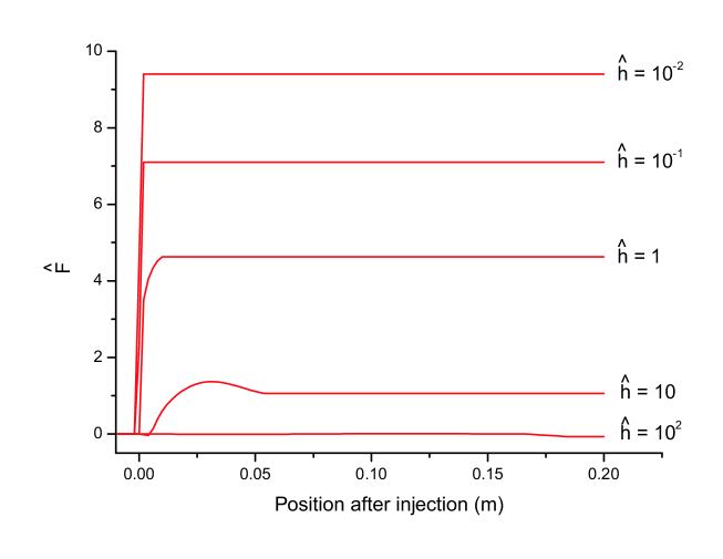
Figure 1: Normalized radial force from the head of the bunch ($\Delta s<0$) to the tail as the bunch progresses inside the bend ($z=0$ corresponds to the injection of the test particle in the magnet). Here $R=1~{}$m and $\gamma=100$. Here we plot the results from TraFiC⁴ for several values of $\hat{h}=h\gamma^{2}/R$, $h$ being the vertical displacement of the test particle. The bunch length is $200\mu m$. The test particle is located in the middle of the bunch.

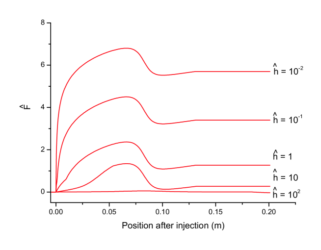
Figure 2: Normalized radial force acting on a test particle from a bunch with rectangular density distribution entering a hard-edge bending magnet as a function of the position of the test particle inside the magnet. The solid lines show analytical results; the circles describe the outcome from TraFiC⁴. We chose $\gamma=100$, $R=1$ m; graphs are plotted for several values of the parameter $\hat{h}=h\gamma^{2}/R$, $h$ being the vertical displacement of the test particle. The bunch length is $200\mu~{}$m. The test particle is located in the middle of the bunch.

Let us spend some words to describe the head-tail interaction (an exhaustive treatment can be found in [9, 10]). On the one hand it is evident that, when $\Delta s<0$, the source particle is ahead of the test electron at any time; on the other hand it is not true that the retarded position of the source particle is, in general, ahead of the present position of the test particle. If $\Delta s<0$ and, approximatively, $|\Delta s|<h$ the test particle overtakes the retarded position of the source before the electromagnetic signal reaches it. In this case, although we may still talk about head-tail interaction, since $\Delta s<0$, its real character is very much similar to the case $\Delta s>0$, in which the electromagnetic signal has to catch up with the test particle. In the case of head-tail interactions with $|\Delta s|>h$, the retardation condition has unique features since the electromagnetic signal runs against the test particle, and not viceversa, as in the tail-head case (or in the head-tail case with $|\Delta s|<h$, when the electromagnetic is running after it. The fact that the electromagnetic signal and the test particle approach on a head-on collision is the reason why the character of this interaction is local, in the sense that the distance which the test particle travels between the emission of the electromagnetic signal by a source and its reception by the test particle is about half of the distance between the test particle and the source, while the usual tail-head interaction has a formation length about $\gamma^{2}$ times longer. This can be seen directly comparing Fig. 1 and Fig. 2.

It is somehow surprising that, although simulations automatically take care of this term, this has been overlooked for a long time in theoretical analysis or in the interpretation of simulation results, starting from [7], continuing with [8], [5] and finally [3]. This important term is responsible for sudden jumps of $\hat{F}$ at the magnet entrance. Consider for example the plot in Fig. 3, obtained by using the electromagnetic solver of $\verb"TraFiC"^{4}$. The figure shows (solid line) the normalized radial force $\hat{F}$ felt by a test particle (this is just the sum of Fig. 1 and Fig. 2) in the middle of the bunch and the normalized potential $\hat{\Phi}=\Phi/[e^{2}\lambda/(4\pi\varepsilon_{0})]$ (dashed line) at the test particle position. The sudden jumps at the magnet entrance are due to head-tail interaction with $|\Delta s|>h$. Yet, before [9, 10], there was no theoretical explanation for this behavior. Although Fig. 3 refers to displacement in the vertical plane, it is obvious that a similar displacement would be found in the horizontal one too, signifying a logarithmic dependence on $x$.

Figure 3: Normalized radial force (solid line) and normalized potential (dashed line) in the center of a 200 $\mu$m bunch as a function of the injection position. The parameter on the curves refers to the vertical displacement $h$ of the test particle.

Now that the head-tail interaction has been introduced, it is possible to give a very simple argument against the meaningfulness of the cancellation scheme. In [3] attention is drawn only on $G_{r}$ and $G_{c}$, while no word is spent about $G_{0}$ and $G_{\|}$. As already said, in Fig 3 we also plotted (dashed lines) the normalized potential $\hat{\Phi}$ in the center of the bunch for different vertical displacements $h$ as calculated by $\verb"TraFiC"^{4}$. As it is seen, the potential does not share the same formation length of the head-tail force, which clearly demonstrates that no effective cancellation can take place between $F_{\bot}$ and $\Delta E$. This fact can be shown in the same terminology used in [3]. Even if $G_{c}$ is negligible and $G_{r}$ is centripetal, there is a huge, dominant centrifugal contribution on the right hand side of Eq. (8): this is $G_{0}$ which includes the term $\Phi(0)/R$. Since the head-tail interaction has local nature, we can say that, due to the rearrangement proposed in [3], $G_{0}$ now includes all the head-tail interaction part (the sharp time dependence of the head-tail interaction being masked in the other terms of Eq. (7), i.e. in the terms $G_{\|}$, $G_{r}$ (and $G_{c}$)).

Actually our result shows that $G_{c}\sim 0$, alone, is uninteresting, that is, the cancellation effect as defined in [3] is uninteresting. There will be anyway a strong head-tail contribution which is accounted in the first term $G_{0}$. Since this term depends on the position of the test particle inside the bunch it will lead to emittance growth both in the transient and in the steady state case. This term has not been taken into account in [7] nor in [8]; it has been automatically included in the simulations in [3], because the computational scheme is correct, although unnecessarily complicated, but then it has been disregarded in the analysis of the results. Note that the first term $G_{0}$ would give a spread similar to that of $F_{\bot}$ in Fig. 1 of reference [3] if plotted for a bunch with a given energy spread, since it depends logarithmically on $x$ (at least in the 1D model with the test particle displaced horizontally). In other words, if there is a field singularity, it is there also in the right hand side of the equation of motion and it cannot be cancelled away. Note that there is no possibility of cancelling $G_{0}$ by choosing a certain initial condition for the bunch. In fact the freedom of choice of the initial condition refers to the kinetic energy deviation from the design energy, and not to the deviation of the total energy (kinetic energy summed to the potential energy) from the design kinetic energy.

This shows that there is no theoretical nor practical reason for adopting the cancellation scheme as a preferred one with respect to the usual scheme of calculating separately $F_{\bot}$ and $\Delta E$. In fact, from a practical viewpoint one will encounter the same computational difficulties and from a theoretical viewpoint two easily understandable terms are mixed up into four terms (of which three survive and one is approximately cancelled) with a more involved physical interpretation. Not to mention that the cancellation method can be extremely confusing. The latter is a statement, not an opinion; in the LCLS Design Study Report [2] we read that all contributions to the the transverse emittance growth are due to the centripetal force ”which originates from radiation of trailing particles and depends on the local charge density along the bunch. The maximum force takes place at the center of the bunch and its effect on the transverse emittance is estimated in the reference.”; the reference in the quoted passage is the work by Derbenev and Shiltsev [5]. Here the head-tail contributions are completely neglected, because of the confusion coming form the cancellation issue: in fact the (centripetal) force in the quote is the third term in Li’s treatment ($G_{r}$, the only one considered) while the first term $G_{0}$, containing the (centrifugal) head-tail interaction and the second, $G\|$, are completely neglected. This is an example where on the one hand the code $\verb"TraFiC"^{4}$ was correctly used giving correct results, but where, on the other hand, its results were completely misunderstood. Nevertheless, as we already said, the head-tail interaction is a few times larger than the tail-head interaction, and, since it depends on the position of the test particle along the bunch, it is obviously responsible for normalized emittance growth.

The cancellation scheme as in [3, 4, 6], actually reduces to the following: get a quantity $A+B$ and express $A=A_{1}+A_{2}$, $B=B_{1}+B_{2}$ where $A_{2}\simeq-B_{2}$, leaving large part of $A$ (and even singular quantities) in $A_{1}$, complicate the situation furthermore breaking $A_{1}+B_{1}$ in several parts and then claim that the cancellation $A_{2}+B_{2}\simeq 0$ is an important finding. This can be done with any pair of quantities $A$ and $B$, and it is, in our view, completely trivial and uninteresting. As a final remark, one could have foreseen that the cancellation effect cannot be of any use since the transverse head-tail force, which has local character cannot be effectively cancelled by the energy deviation, which depends upon all the trajectory.

5 Conclusions

In this paper we proved that the cancellation effect is an artificial one. In the right hand side of the transverse equation of motion the Lorentz force and the kinetic energy deviation from the design energy, which are clearly physically meaningful quantities, are combined together to give four different terms of difficult physical interpretation. The cancellation effect deals only with one of these terms, still leaving other three important contributions to be evaluated. We found in [9, 10] that the head-tail interaction is, in practical situations, a few times larger than the tail-head interaction. This fact, automatically included in computer simulation, has always been forgotten in analytical considerations, starting from [7] on. The formation length of the head-tail interaction with $|\Delta s|>h$ is approximately half of the bunch length, which means that, for practical purposes, the head-tail interaction has a local nature. This explains the sudden ”jump” in the total Lorentz force seen as a bunch enters a bending magnet. On the other hand, the kinetic energy deviation from the design energy has much a larger formation length. This fact alone is sufficient to prove that the cancellation effect is an artificial one, in that an important contribution (the head-tail interaction) cannot be compensated by the potential term in the kinetic energy deviation.

When we state that the cancellation effect is artificial, we do not mean that it is, strictly speaking, wrong; we simply state that it is not useful at all and that there is no theoretical nor practical reason to prefer this method to the more straightforward approach of calculating, separately, the transverse Lorentz force and the kinetic energy deviation term (as, for example, by means of the code $\verb"TraFiC"^{4}$). In fact, from a practical viewpoint one will encounter the same computational difficulties and from a theoretical viewpoint two easily understandable terms are mixed up into four terms (of which three survive and one is approximately cancelled) with a more involved physical interpretation.

6 Acknowledgements

We wish to thank Martin Dohlus for providing numerical calculations using the code $\verb"TraFiC"^{4}$. Also, thanks to Joerg Rossbach and Marnix van der Wiel for their interest in this work.

References

- [1] TESLA Technical Design Report, DESY 2001-011, edited by F. Richard et al., and http://tesla.desy.de/
-
[2]
The LCLS Design Study Group, LCLS DEsign Study Report, SLAC
reports SLAC- R521, Stanford (1998) and
http:
www-ssrl.slacstanford.edu/lcls/CDR - [3] R. Li, in Proceeding of the EPAC2002 Conference, Paris
- [4] C. Bohn, FERMILAB-Conf-02/138-T, 2002
- [5] Y. Derbenev and V. Shiltsev, in Fermilab-TM-1974 (1996)
- [6] R.Li, Y. Derbenev, JLAB-TN-02-054
- [7] R. Talman, Phys. Rev. Letters, 56, 14, p. 1429 (1986)
- [8] E. P. Lee, Particle Accelerators, 25, 241 (1990)
- [9] G.Geloni, J. Botman, J. Luiten, M. v.d. Wiel, M. Dohlus, E.Saldin, E.Schneidmiller, M.Yurkov, DESY 02-48 (2002)
- [10] G.Geloni, J. Botman, M. v.d. Wiel, M. Dohlus, E.Saldin, E.Schneidmiller, M.Yurkov, DESY 03-44 (2002)
- [11] E. L. Saldin, E. A. Schneidmiller and M. V. Yurkov, Nucl. Instr. Methods A 398, 373 (1997)