Response of Autonomic Nervous System to Body Positions: Fourier and Wavelet Analysis

Abstract

Two mathematical methods, the Fourier and wavelet transforms, were used to study the short term cardiovascular control system. Time series, picked from electrocardiogram and arterial blood pressure lasting 6 minutes, were analyzed in supine position (SUP), during the first (HD1), and the second half (HD2) of $90^{\circ}$ head down tilt and during recovery (REC). The wavelet transform was performed using the Haar function of period $T=2^{j}$ ($j=1$,$2$,$\cdots$,$6$) to obtain wavelet coefficients. Power spectra components were analyzed within three bands, VLF (0.003-0.04), LF (0.04-0.15) and HF (0.15-0.4) with the frequency unit cycle/interval. Wavelet transform demonstrated a higher discrimination among all analyzed periods than the Fourier transform. For the Fourier analysis, the LF of R-R intervals and VLF of systolic blood pressure show more evident difference for different body positions. For the wavelet analysis, the systolic blood pressures show much more evident difference than the R-R intervals. This study suggests a difference in the response of the vessels and the heart to different body positions. The partial dissociation between VLF and LF results is a physiologically relevant finding of this work.

I Introduction

I.1 Physiological background

Like all other animals, human body must monitor and maintain a constant internal environment. At the same time, it must monitor and respond to the external stimulus. Two integrated and coordinated organ systems, the nervous system and the endocrine system, are responsible for these two functions. The nervous system monitors and controls nearly every organ system through a series of positive and negative feedback loops. The central nervous system includes the brain and spinal cord. The peripheral nervous system connects the central nervous system to the other parts of the body. There are two subdivisions in the peripheral nervous system, the somatic and the automnomic. The somatic nervous system includes all nerves controlling the skeletal muscular system and external sensory receptors. The somatic nervous system is involved in voluntary control. The autonomic nervous system is that part of the peripheral nervous system which controls internal organs which are not under conscious control. The autonomic nervous system has two subsystems, sympathetic and parasympathetic. The sympathetic nervous system is involved in response to stress conditions. The parasympathetic is involved in relaxation. Each of these subsystems usually operates in the reverse of the other. Many organs are innervated by both of them, and their levels of activity are reciprocally balanced to maintain homeostasis.

The autonomic nervous system controls muscles in the heart. It directly controls the cardiovascular system, both of its electrical and mechanical properties. Via its excitation, inhibition and modulation, it regulates both the heart rate and the propagation of cardiac electrical activity. The autonomic nervous system controls a wide range of variables, including arterial pressure, cardiac output, blood flow, and vasomotor tone. It is responsible for the immediate response of the heart and the blood vessels to internal noise courses as well as external perturbations. The former includes respiration, digestion, emotion, and etc. The latter includes body posture, physical activity, temperature, and others.

In a healthy individual, the beat-by-beat adjustment of hemodynamic parameters by the autonomic nervous system is essential to an adequate cardiovascular functioning. Therefore, cardiovascular control, as expressed by the time-dependence of hemodynamic variables, is a direct reflection of autonomic activity. It may be used as a probe of autonomic performance or maturation and a detector of possible autonomic malfunction.

Spectral analysis of variablity in heart rate and blood pressure provides a quantitative noninvasive means of assessing the functioning of the short-term cardiovascular control systems. Sympathetic and parasympathetic nervous activity makes frequency-specific contributions to power spectrascience1981 of heart rate and blood pressure.

I.2 Motivation and objectives

Due to the regulation mentioned above, one can design experiments relating to internal noises and/or external perturbations to investigate the responsiveness of autonomic nervous system. This is the basic motivation and objective of the research in this line. Many interesting results have been achievedReview1 ; ConPhys ; Review2 ; time-interval . The present research was made on commitment of Italian Soccorso Alpino e Speleologico (a group of volunteer helpers for rescue in difficult environments) to study body changes in helpers who often must go in head-down positions to rescue wounded persons in caves or under ruins of crushed buildings. Specific objective of this research is to study the response of autonomic nervous system to body positions by spectral analysis of both heart rate variability and systolic blood pressure.

The structure of the following part of this paper is as follows: In Sect. II we describe the methods used in this research, which include how we chosed the subjects, how recorded the physiological signals, how picked out time-series for the further study, numerical tools and statistics. Section III gives the numerical results and physiological interpretations, which is the core of this paper. We draw a conclusion in Sect. IV.

II Methods

II.1 Subjects and database

We studied nine male subjects (33$\pm$5.7 years old) labelled as DE, GI, LO, PI, PS, RA, SA, SC, and TA, respectively. For each subject we recorded the electrocardiogram (ECG) and the blood pressure (BP) signals for consecutive four times. The BP signals was obtained by photoplethysmographic recording of a sphygmogram at a finger of the right hand, maintained throughout all the experiment at the same hydrostatic level as the heart. The initial status is supine and the recording time is $6$ minutes (SUP). Then the body position of the subject was slowly, in about 20 seconds, tilted to $90^{\circ}$ head down (HD). Just after the transition of body posture, a second set of signals of $6$ minutes (HD1) was recorded. After that keeping the head down position for about $10$ minutes, then a third set of signals of $6$ minutes (HD2) was recorded. Finally the body position of the subject was slowly recovered to supine and the fourth set of signals of $6$ minutes (REC) was recorded.

The lower frequency limit 0.02 Hertz (Hz), corresponding to the higher period limit 50 seconds, is typical and adequate for human adults when performing short-term spectral analysis. A generally accepted trace length should contains approximately five full periods of the slowest investigated fluctuationtrace . Our data length is about 360 seconds. The sampling rate is 1000 Hz. So both the sampling rate and the trace length are acceptable.

II.2 PQRST Sequence and time-series

Readily recognizable features of the ECG wave pattern are designated by the letters P, Q, R, S, and T. The wave itself is often referred to as PQRST or QRS complex. Aside from the significance of various features of the QRS complex, the timing of the sequence of the QRS complexes over tens, hundreds, and thousands of heart beats is also significant. These inter-complex times are readily measured by recording the occurrences of the peaks of the large R waves. The number of R-R intervals within one minute is the generally called heart rate. From the ECG, the R-R intervals compose our original time-series $\{\tau_{i}\}$, where $i$ is the index of the R peak or the index of the R-R intervals. Similarly, from the blood pressure, the systolic blood pressures (SBP) compose our original time-series $\{y_{i}\}$, where $i$ is the index of the peak of SBP or the index of the SBP-SBP intervals. Here we stress the original to distinguish them from the resampled ones. Our numerical tools, Fourier transform and wavelet transform, require that the time series be evenly distributed. From the interval-based point of view time-series $\{\tau_{i}\}$ and $\{y_{i}\}$ are evenly distributed, while from the time-based point of view, $\{\tau(t_{i})\}$ and $\{y(t_{i})\}$ are unevenly distributed. The two kinds of time-series describe the same physiological process in a little different ways. If one wants to use the time-based time-series for spectrum analysis, he needs to resample them. In this research the used resampling time interval is 0.25 second, which results in a Nyquist critical frequencyRecipe $2$ Hz. One must care the correspondence of the frequency unit and that of the used time-series. If one uses the interval-based time-series, the frequency unit is cycles/interval. If one uses time-based time-series, the frequency unit is cycles/(time unit). If the time unit is second, then the frequency unit is Hz. For typical interbeat interval sequences, the two kinds of frequency units are correlated by a formulatime-interval

$$f_{time}=f_{interval}/E[\tau]\text{,}$$ (1)

where $E[\tau]$ represents expectation value of the R-R intervals, $f_{time}$ and $f_{interval}$ are respectively the time-based and the interval-based frequency. The values of $E[\tau]$ for all subjects and the four body positions are shown in Table I. The mean value of systolic blood pressure is also an important measure for the body conditions. The corresponding values are shown in Table II.

Table I: Mean R-R intervals for different subjects and different body positions. The time unit is second.

subject index 1 2 3 4 5 6 7 8 9

SUP 0.79 0.97 1.10 0.99 0.83 1.20 1.07 0.83 1.08

HD1 0.75 0.97 1.11 1.05 0.91 1.05 1.01 0.81 1.07

HD2 0.77 0.97 1.00 1.04 0.89 1.09 0.93 0.82 1.06

REC 0.86 1.13 1.15 1.07 0.91 1.21 1.08 0.96 1.10

Table II: Mean values of the systolic blood pressure for different subjects and different body positions. The unit is mmHg.

subject index 1 2 3 4 5 6 7 8 9

SUP 122 110 106 122 118 108 120 121 122

HD1 118 123 110 123 116 134 107 116 115

HD2 119 123 107 121 120 134 105 122 113

REC 128 116 107 126 118 103 116 116 132

II.3 Fourier transform

The spectral analysis based on Fourier transform is by far the most used quantitative method for the analysis of physiological signals. Moreover, it has reached importance as a diagnostic tool. Fourier transform allows the separation and study of different rhythms which are intrinsic for the physiological signals. It makes simple a task that is difficult to perform visually when several rhythms occur simultaneously.. The following is the definition of the discrete Fourier transform used in the present research,

$$\tilde{x}_{k}=\frac{1}{\sqrt{N}}\sum_{j=0}^{N-1}x_{j}\exp(i\frac{2\pi}{N}jk)\text{,}$$ (2)

where $\{x_{j}\}$ is the used time-series and $\{\tilde{x}_{k}\}$ is the corresponding Fourier transform, $N$ is the number or length of the time-series. With this definition, what the power spectrum shows is mean contribution of each data in the time-series. From the statistical point of view, the power spectrum is independent of the length of the time-series if it is stable during the measuring time. In fact the nonstationarity generally exists if the measuring time is long. But the present research is focused on short term cardiovascular control system. A drawback of the traditional Fourier transform is that one can not observe the time behavior of the specific frequency components. This defect is partially resolved by using the Gabor transformGabor , also called short time Fourier transform, which first modulates the time-series with an appropriate window function, then performs the Fourier transform. The window function peaks around a given time and falling off rapidly, thus emphasizing the signal localized at the central and suppressing the distant times. If one shifts the window along the time, the time behavior will be observable.

II.4 Wavelet transform

The Gabor transform still has a defect, the window width is fixed. In recent years physiological time series have been considered in a more general framework of fractal functions. See, e.g. Nature . An extensively used method in this kind of studies is the wavelet transformwavelet , with which the window width is also adjustable. Wavelet analysis has proved to be a useful technique for analyzing signals at multiple scalesw1 ; w2 ; w3 ; w4 ; TeichPRL ; PRL812388 ; Sebino . It permits the time and frequency characteristics of a signal to be simultaneously examined, and has the advantage of naturally removing polynomial nonstationarities.

The continuous wavelet transform maps a signal with one independent variable $t$ onto a function with two independent variables, $a$ and $b$. This procedure is redundant and not efficient for algorithm implementations. A more practical and convenient choice is to use a dyadic discrete wavelet transform. For the sequence $\{\tau_{i}\}$, it is defined as follows,

$$W_{m,n}=\frac{1}{\sqrt{m}}\sum_{i=0}^{N-1}\tau_{i}\psi(\frac{i}{m}-n)\text{, }$$ (3)

where the quantity $\psi$ is the wavelet basis function, and $N$ is the length of the time-series, $m$ is scale which is related to the scale index $j$ by $m=2^{j}$, and $n$ is the translation variable. The interpretation of wavelet coefficients depends on the shape of the basis function. Both $j$ and $n$ are nonnegative integers. The term dyadic refers to the use of scales which are integer powers of $2$. This is an arbitrary choice. The wavelet transform could be calculated at arbitrary scale values, although the diadic scale enjoys some convenience of mathematical propertiestime-interval ; w2 . In this research we used the Haar wavelet,

$$\psi_{Haar}(t)=\left\{\begin{array}[]{ll}-1&\text{for }0\leq t<0.5\text{, }\\ 1&\text{for }0.5\leq t<1\text{, }\\ 0&\text{otherwise. }\end{array}\right.$$ (4)

which has been used in some physiological signals analyses. [For example, see Ref. Sebino .] An extensively used measure devised from the wavelet transform is the standard deviation of the wavelet coefficients as a function of scaletime-interval :

$$\sigma(m)=\left[\text{E}\left\{|W_{m,n}(m)-E[W_{m,n}(m)]|^{2}\right\}\right]^{1/2}\text{,}$$ (5)

where the expectation is taken over the time-series, and is independent of $n$. In Ref.Sebino the Haar wavelet is shown to be suitable for scale-dependent measures of $\sigma$.

II.5 Frequency bands

The periodogram covers a broad range of frequencies which can be divided into bands that are relevant to the presence of various cardiac pathologies. The power within each band is calculated by integrating the power spectral density over the associated frequency range. The divisions of frequency bands in the literatures are not exactly the same. A commonly used division in heart rate variability (HRV) is shown in Table IIItime-interval , where VLF means the band of very low frequencies, LF means the band of low frequencies, HF means the band of high frequencies. The unit for this table is cycle/interval. So the boundaries of frequency bands have a shift with the mean value of the R-R intervals, thus are related to specific subject and specific body conditions. In this research we used this division. Under the context without ambiguity, VLF, LF and HF are also used to denote the powers of corresponding frequency bands. The power of VLF maybe correlated to the oscillations of blood vessels. The power of LF may reflect both the sympathetic and parasympathetic activities. Efferent parasympathetic activity is a major contributor to the power of HFtime-interval .

Table III: A division of frequency bands. The frequency regime is divided into three bands, very low frequencies (VLF), low frequencies (LF), and high frequencies (HF). The unit for this table is cycle/interval.

VLF 0.003-0.04

LF 0.04-0.15

HF 0.15-0.4

II.6 Statistics

To evaluate the performance of different measures, one needs to do some statistics. Comparisons among the four successive body positions, SUP, HD1, HD2 and REC, are first performed by an ANOVA (analysis of variance) test for repeated measures. The ANOVA test takes into account not only changes in mean values and standard deviation, but also changes occurring in each subject in different experimental conditions. This test is considered significant when $p<0.05$, where $p$ is the probability that the data contained in the four groups of measures are not different, but they are randomly extracted from the same pool of data. It is commonly accepted in biological measurements that, if such a probability is less than $5\%$, the different groups of measures can not be considered as randomly extracted from the same pool, but some real difference does exist among them. This procedure should first be employed when comparisons are made among three or more groups of measures, due to mathematical considerations about the interdependence of the measures in different groups and their degree of freedom. In other words, it is commonly accepted that, if we have three or more groups of measures we can not immediately compare them two-by-two, but an overall assessment of the variance must be made first. If the ANOVA test gives a $p$ value less than $0.05$, special post-ANOVA tests can be made to compare two-by-two each group of measures with the others. If the ANOVA test gives a $p$ value larger than $0.05$, we can not get much meaningful information from it. But the t-test-2 analysis still can be used to compare measures of each two of the four groups.

T-test-2 is a hypothesis testing for the difference in means of two samples. We used the software, MATLAB, for these statistic computations. For two samples, ${\bf x}$ and ${\bf y}$, t-test-2 in MATLAB presents three quantities, h, significance and ci. The value of h is a t-test to determine whether two samples from a normal distribution in the samples could have the same mean when the standard deviations are unknown but assumed equal. The result is $h=1$ if you can reject the null hypothesis at the 0.05 significance level, and is $h=0$ otherwise. In this research, $h=1$ means that significant difference is found from different body positions. The significance is the $p$-value associated with the T-statistic

$$T=\frac{{\bf\bar{x}}-{\bf\bar{y}}}{s\sqrt{\frac{1}{n}+\frac{1}{m}}}\text{, }$$ (6)

where $s$ is the pooled sample standard deviation, $n$ and $m$ are the numbers of observations in the ${\bf x}$ and ${\bf y}$ samples, and ${\bf\bar{x}}$ and ${\bf\bar{y}}$ are the corresponding expectation values. The value of significance is the probability that the observed value of $T$ could be as large or larger by chance under the null hypothesis that the mean of ${\bf x}$ is equal to the mean of ${\bf y}$. The quantity ci is a 95% confidence interval for the true difference in means. In fact in present research, the t-test-2 analysis was done for any value of $p$ from the ANOVA. In the case of the ANOVA $p<0.05$, t-test-2 plays a similar role to that of the post-ANOVA.

III Results and discussions

III.1 Fourier analysis

Before the Fourier transform, we first used the Hamming window functionhamming to modulate the time-series, then subtracted the mean value and rescaled the time-series so that the mean value is zero and the standard deviation is $1$. The powers of VLF, LF and HF are averaged over different shifts of the window function. For Fourier transform of the resampled time-series, the used window width is $256$ seconds ($1024$ points). For Fourier transform of the original interval-based time-series, the used window width is $256$ intervals.

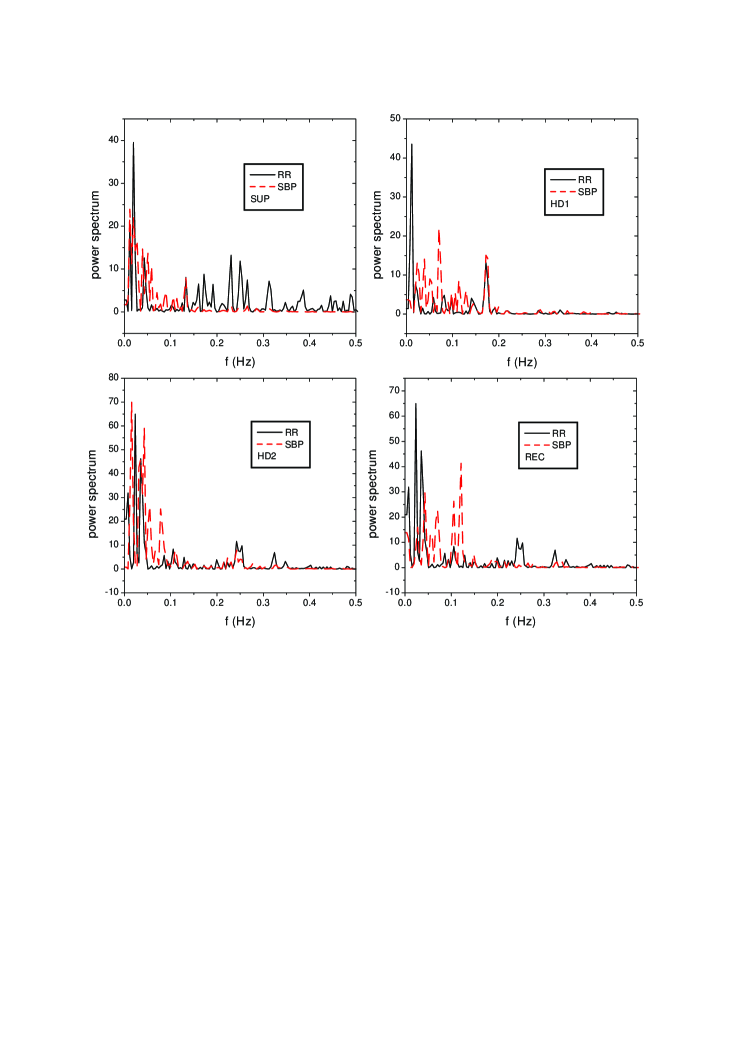
Figure 1: Power spectra of the R-R intervals and the systolic blood pressures for the subject “DE” for the four seccessive body positions. The corresponding body positions are shown in the insets of the figure.

Figure 1 shows the power spectra of a subject for the consecutive four body status. Here we used the resampled time-based time series, so the frequency unit is Hz. In each case, the solid line is for the R-R intervals and the dashed line is for the systolic blood pressure. The status of the body position is also shown in the inset of each figure. It is clear that (i) the most of power is localized with the frequency regime $0<f<0.4$, (ii)the contribution of different frequency components varies with different body positions. For the R-R intervals of this subject, the power in the low frequency part decreased during the transition from SUP to HD1, and increased from HD1 to HD2. The behavior of the systolic blood pressure are not exactly the same as that of the R-R intervals. The power spectra for different subjects show evident difference which may due to personal conditions as well as respiratory status. That is beyond the scope of the studies described in this paper. What one cares is not the specific values, but the mean value and its statistics. The power spectra from the original interval-based time-series give similar information.

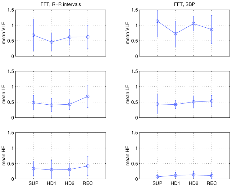
Figure 2: Mean values of VLF, LF and HF with error-bars. The first column is for the R-R intervals and the second column is for the systolic blood pressures. The same scales are used in each case for the convenience of comparison.

Figure 2 shows the mean values of VLF, LF and HF for different body positions, where the first column is for the R-R intervals and the second column is for the systolic blood pressures. The error bars are also shown for comparison. These results are from the resampled time-based time-series. From the two figures, it is clear that the VLF for both the R-R intervals and the systolic blood pressure has a significant decrease when the body position changes from supine to $90^{\circ}$ head down, while decrease of LF for both is less evident. A physiological interpretation is thus: when the body position changes from supine to head down, due to the weight of the column of blood lending from feet to the heart and the neck, the arterial pressure sensors, which are in the aorta near the heart and in the neck, get a strong stimulation. This is very similar to a sudden hypertension and induces a negative feedback response. The sympathetic activity on the heart and the vessels is inhibited, while the parasympathetic activity on the heart is increased. The inhibition of sympathetic activity induces different effects: (i) decreasing the ability of the heart wall to increase its elastance during systole, which tends to decrease the systolic blood pressure; (ii) a dilation of vessels which decreases the Poiseuille resistance to the blood, which tends to lengthen the R-R intervals. The parasympathetic activity does not significantly affect the resistance of vessels. So for both the R-R intervals and the systolic blood pressures, the decrease in the variability of very low frequency components can be connected to the decrease in physiological very slow oscillations in sympathetic activity. In HD1 status those very slow oscillations seem to be heavily dampened by the feedback effects elicited by the hydraulic mass which is stretching pressure receptors. It is also very interesting that these effects is not so evident in the variability of low frequency components of R-R intervals and systolic blood pressures. This could suggest that systems whose oscillations have longer time constants are more influenced by changes in hydraulic dislocations than the more rapidly oscillating systems. The contribution of a longer oscillation period is mainly from the peripheral vessels, whose slow oscillations in resistance affect not only blood pressures, but also, in a reflex way, the R-R intervals.

After the SUP-HD1 transition the changes are reduced in the HD2 status. This agrees with a progressive decay in the arterial pressure receptors sensitivity, which is known to be significantly reduced after 10-15 minutes of application of a constant mechanical stimulus. However, during the HD2 period, a great volume of blood has been transferred from the more elevated parts of the body (for example, legs) to the thorax, so that the recovery from the HD2 status to the REC has the effect to suddenly displace this hydraulic mass towards the vasodilated vessels of the legs. This mimicks a sudden hypotension as in blood losses due to hemorrhage. The sympathetic activity is enhanced as if it should counteract the effects of a hemorrhage. So the variability in very low and low frequency components of R-R intervals becomes higher than in HD1 status, and the variability of low frequency components also becomes higher than in HD2 status. This again suggests a difference in the response of the vessels (mainly VLF, due to longer time constant of their oscillations) and the heart (mainly LF, due to shorter time constants of heart rate and contractility oscillations).

Because the low frequency oscillations are influenced by both sympathetic (vessels and heart) and parasympathetic (heart only) systems, it seems that very low frequency variability is more greatly dampened and “stunned” by head-down position than the low frequency variability. That is to say, the low frequency components of systolic blood pressure recovers more promptly during the REC period than the very low frequency components. This behavior suggests that the recovery of systolic blood pressure is mainly supported by recovery in heart rate and contractility, but not in peripheral vessels resistance whose VLF power remains low.

For the systolic blood pressure, the variability of high frequency components in both the HD and the REC status are higher than that in the initial supine position. This can only be a parasympathetic effect (perhaps influenced by an increase in respiratory activity in head-down position). For the R-R intervals, the behavior is not exactly the same.

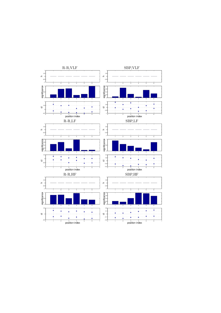
Figure 3: T-test-2 analysis results of VLF, LF, and HF for any position-pair of the four body positions. The first column is for the R-R intervals and the second column is for the systolic blood pressures. The position indexes 1,2,3,4,5,6 correspond to the position-pairs SUP-HD1, SUP-HD2, SUP-REC, HD1-HD2, HD1-REC, HD2-REC, respectively.

For the Fourier analysis, Table IV shows the $p$ values from the ANOVA analysis for the three measures, VLF, LF and HF. All the $p$ values are larger than $0.05$. So this table suggests that for any one of the three measures, among the four successive body positions, no one shows significant difference from the other three under the significance level $0.05$. The R-R intervals and systolic blood pressures are facing the same situation at this point. But the LF of R-R intervals and the VLF of systolic blood pressures are expected to be observed more difference because their $p$ values are relatively smaller. Let us go to the t-test-2 analysis. Figure 3 shows the t-test-2 statistic results for any two of the four different body positions. The first column is for the R-R intervals and the second column is for the systolic blood pressures. From top to bottom, the corresponding frequency bands are VLF, LF and HF. The position indexes 1, 2, 3, 4, 5, 6 correspond to SUP-HD1, SUP-HD2, SUP-REC, HD1-HD2, HD1-REC, HD2-REC, respectively. We found that all the $p$ values from the t-test-2 are larger than $0.05$, so the corresponding values of $h$ are all zero. But from the LF of R-R intervals, two pairs of body-positions, HD1-REC and HD2-REC, show relatively smaller $p$ values. That tells us that the REC shows evident difference from both the HD1 and the HD2 in the LF of the R-R intervals, which is consistent with what we got and understood from Fig. 2. From the VLF of systolic blood pressure, SUP-HD1 and HD1-HD2 show relatively small $p$ values, which also confirms again what we got from Fig. 2.

Table IV: The ANOVA $p$ values of different measures of the power spectra. Results for the R-R intervals and for the systolic blood pressures are shown.

VLF LF HF

R-R 0.62 0.10 0.76

SBP 0.18 0.63 0.53

III.2 Wavelet analysis

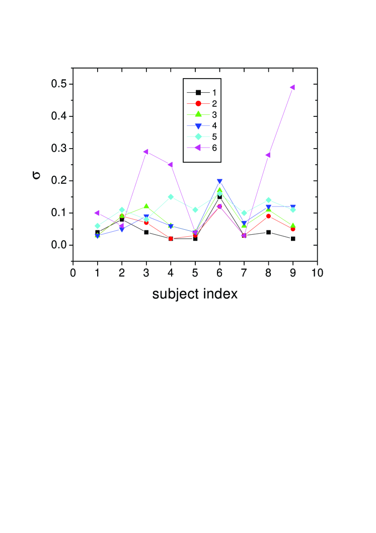
Figure 4: Standard deviation of the wavelet coefficients as a function of scale index and subject index. The corresponding scale indexes are shown in the inset. This result is for the supine position.

In this section we mainly describe the wavelet analysis on the original interval-based time-series. The wavelet function is the Haar wavelet. The used the scale $m=2^{j}$. Since the used window width is $1$, the scale index $j$ approximately corresponds the frequency $1/2^{j}$ cycle/interval. From Table I we know that the mean R-R interval of the nine subjects is $0.98$ second in SUP, is $0.97$ second in HD1, is $0.95$ second in HD2 and is $1.05$ second in REC. So we can approximately evaluate the frequencies corresponding to different scale indexes. The correspondences are shown in Table V. Figure 4 shows the standard deviation $\sigma$ of the wavelet coefficients as a function of the scale index $j$ and the subject index. The scale indexes are shown in the inset of the figure. For the same subject the value of $\sigma$ varies with the scale, and for the same scale the value of $\sigma$ also oscillates with specific subject. This result is for the initial SUP.

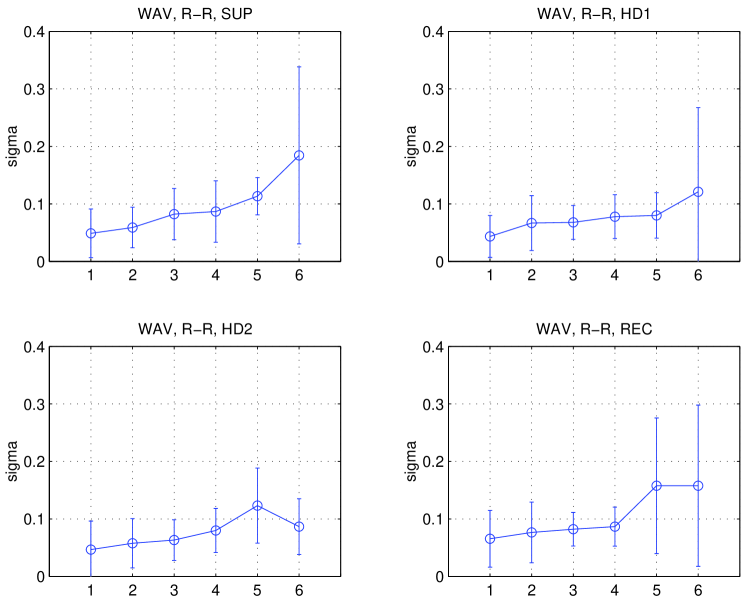
Figure 5: Mean value of the standard deviation of the wavelet coefficients with error-bars as a function of scale index $j$. This result is for the R-R intervals.

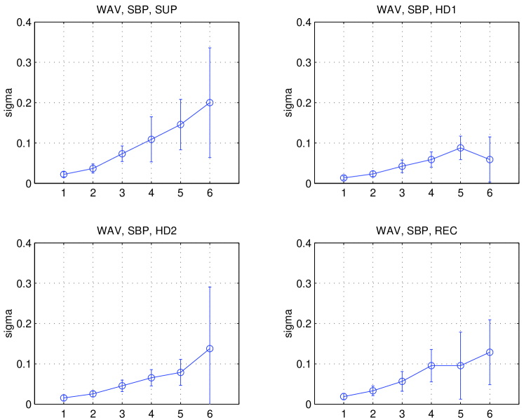
Figure 6: Mean value of the standard deviation of the wavelet coefficients with error-bars as a function of scale index $j$. This result is for the systolic blood pressures.

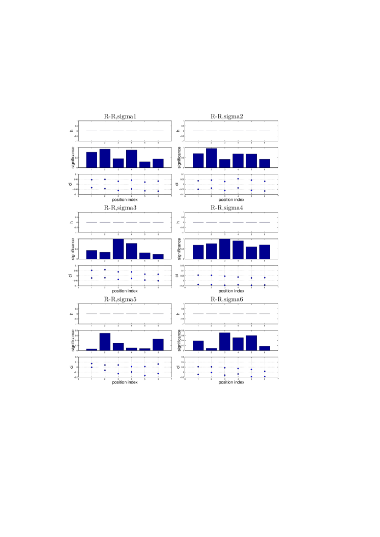
Figure 7: T-test-2 results of $\sigma$ of the six used scales for any position-pair of the four body positions. “sigma1”, …, “sigma6” in the figure correspond to scale indexes 1, …, 6, respectively. The position indexes 1,2,3,4,5,6 correspond to the position-pairs SUP-HD1, SUP-HD2, SUP-REC, HD1-HD2, HD1-REC, HD2-REC, respectively. This result is for the R-R intervals.

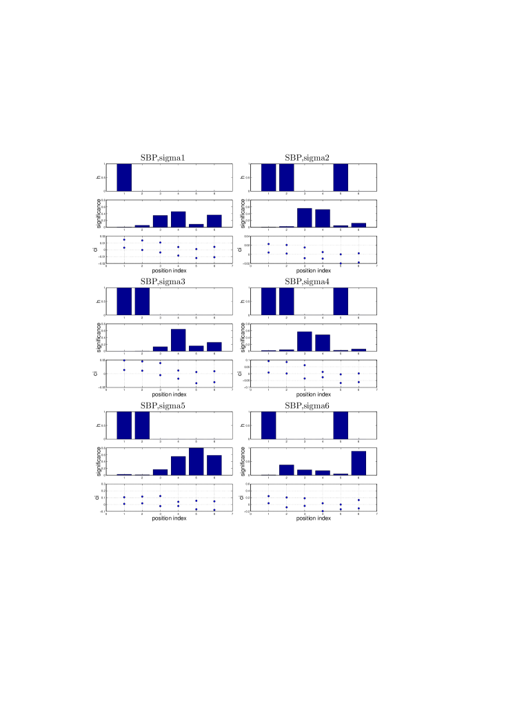
Figure 8: T-test-2 results of $\sigma$ of the six used scales for any position-pair of the four body positions. “sigma1”, …, “sigma6” in the figure correspond to scale indexes 1, …, 6, respectively. The position indexes 1,2,3,4,5,6 correspond to the position-pairs SUP-HD1, SUP-HD2, SUP-REC, HD1-HD2, HD1-REC, HD2-REC, respectively. This result is for the systolic blood pressures.

To get a statistical information on how $\sigma$ behaves as a function of specific scales, Fig.5 shows the mean value of $\sigma$ of the R-R intervals averaged over different subjects. The results for the four body positions are shown in order. The corresponding error-bars are also shown. Figure 6 shows the same quantities but for the systolic blood pressures. During the SUP period, the values of $\sigma$ for both the R-R intervals and the systolic blood pressures show a similar behavior. They increase with the used scale. Let us understand this result. A larger scale corresponds to an oscillation with lower frequency. A larger value of $\sigma$ means that the strength of the oscillation with a given frequency changes more significantly with time. This result suggests that the organs in charge of lower frequency oscillations are more easily affected by other disturbance, so the corresponding oscillations show more nonstationarity with time. This figure also suggests that the nonstationarities of nearly all the frequency components denoted by $j$ were lower in the HD1 and the HD2 periods than in the supine period. In other words, the corresponding oscillations are more stable in the HD1 and the HD2 than in the SUP. From the physiological side, it seems that when the body is receiving a constant mechanical stimulus, some other weak internal noise or external disturbance is less effective in affecting the short term cardiovascular control system. Table VI shows the significance values from the ANOVA analysis. Figures 7 and 8 show, respectively, the t-test-2 results for the R-R intervals and the systolic blood pressures. The correspondences between the position index and the position-pairs are the same as those in Fig.3. For the R-R intervals, all the ANOVA $p$ values are greater than $0.05$, while from the t-test-2 we still can find evident difference for three sets of body positions, SUP-HD1, HD1-HD2, HD1-REC, from scale $j=5$, and can find evident difference from SUP-HD2 from the scale $j=6$, even though the t-test-2 $p$ values are larger than $0.05$. These results are consistent with those of the Fourier analysis. For the systolic blood pressures, all the ANOVA $p$ values are small. That is to say, at least one of the four is evidently different from the other three. For the scales with $j=1,2,3,4$, $p<0.05$. The further t-test-2 gives more detailed information. Under the condition of t-test-2 $p<0.05$, (i) when $j=1$, evident difference is found in SUP-HD1; (ii) when $j=2$ or $4$, evident differences are found in SUP-HD1, SUP-HD2, and HD2-REC, (iii)when $j=3$ or $5$, evident differences are found in SUP-HD1 and SUP-HD2, (iv)when $j=6$, evident differences are found in SUP-HD1 and HD2-REC.

It should be mention that we also used the original interval-based time-series for Fourier analysis and used the resampled time-series for wavelet transform. But these two treatments are less effective in distinguishing different body positions.

Table V: The approximate correspondences between the scale indexes and component frequencies. The unit of frequency here is Hz. The correspondence changes with subject and body positions because the mean R-R interval changes.

scale index 1 2 3 4 5 6

SUP 0.510 0.255 0.128 0.064 0.032 0.016

HD1 0.515 0.258 0.129 0.064 0.032 0.016

HD2 0.526 0.263 0.132 0.066 0.033 0.016

REC 0.476 0.238 0.119 0.060 0.030 0.015

Table VI: Significance values from the ANOVA for different scales of the wavelet transform.

scale index 1 2 3 4 5 6

R-R 0.726 0.799 0.561 0.954 0.171 0.416

SBP 0.047 0.019 0.006 0.021 0.075 0.093

IV Conclusion

We used two methods, the Fourier and wavelet transforms, to analyze arterial blood pressure and heart rate temporal series recorded in four successive body positions. The $90^{\circ}$ head-down position is used in this research. For the Fourier analysis, three measures, VLF, LF and HF, were used. For the wavelet analysis, the standard deviation of the wavelet coefficients for different scales were used. The two mathematical methods are shown to be complementary to study given physiological signals. Time series lasting 6 minutes were analyzed with both methods in supine position (SUP), during the first (HD1), and the second half (HD2)of head down tilt and after recovery (REC). The wavelet transform was performed using the Haar function of period $T=2^{j}$ ($j=1$,$2$,$\cdots$,$6$) to obtain wavelet coefficients. Power spectra components were analyzed within three bands, VLF (0.003-0.04), LF (0.04-0.15) and HF (0.15-0.4 ) with the frequency unit cycle/interval. In distinguishing two different body positions, the resampled time-based time-series work more effectively if we use the Fourier transform, while the original interval-based time-series work more effectively if we use the wavelet transform.

Power spectra mean values showed that (i) the HF components of blood pressure have an increases during tilt and have a decrease during recovery; (ii) LF components of R-R intervals and systolic blood pressures increase in recovery with respect to the tilt period; (iii) VLF components of the R-R intervals and systolic blood pressures were lower in HD1 than in supine position, but increased in HD2; (iv)in recovery period VLF components of R-R intervals return nearly to the supine value, but VLF components of blood pressure decrease during recovery with respect to during both the supine and the HD2. Wavelet transform demonstrated a higher discrimination among all analyzed periods than the Fourier transform, especially for the systolic blood pressures. The oscillations of each frequency component denoted by $j$ of the R-R intervals and the systolic blood pressures were lower in HD1 and HD2 with respect to in SUP. For the Fourier analysis, LF of R-R intervals and VLF of systolic blood pressure show more evident difference for different body positions. For the wavelet analysis, the systolic blood pressures show much more evident difference than the R-R intervals. These data suggest a difference in the response of the vessels and the heart to different body positions. So the R-R intervals and the systolic blood pressures are also complementary in reflecting the response of autonomic nervous system. The partial dissociation between VLF and LF results is a physiologically relevant finding of this work.

As reported above, this research was committed to assess potential risk factors due to cardiovascular changes in helpers working in head-down position to rescue persons entrapped in difficult environments. Physiological oscillations of SBP and R-R intervals in the VLF, LF and HF bands are due to the time constants of the feedback loops regulating these parameters. On the background of a proper amount of ongoing oscillatory activity, the feedback regulation of cardiovascular system is more easily allowed to compensate for the effects of external or internal abrupt perturbations (accelerations, environmental temperature, emotions, fatigue, etc.) on arterial pressure science1981 ; Review1 ; ConPhys ; Review2 ; time-interval ; trace . In physiological terms, if cardiovascular feedback control loops were not continuously oscillating, they would buffer perturbations in a less ready, adaptive and effective way, as it often occurs, for instance, in diabetes and other pathologies affecting the fibers of the autonomic nervous system innervating the heart and the vessels.

The dampening in SBP and R-R oscillations we have found in head-down position likely reflects limitations in adaptive properties, readiness and effectiveness of the cardiovascular control systems, which arises when the blood pressure sensors in aorta and carotid artery are overcharged by the mass of the blood column unusually accelerated from the feet towards the thorax and the neck. Another point to consider is that such a dampening mainly occurs in the VLF band for SBP, which largely depend on changes in capacitance and resistance of arteries, but it mainly occurs in LF band if R-R intervals are considered, which clearly reflects heart period. To efficiently transfer hydraulic power from the heart to the arteries, a proper coupling is required between the heart period and the mechanical time constant of the elastic arteries, which depends on their capacitance and resistance. An uncoupling between the control mechanisms of these two parameters in head-down position is suggested by the finding that SBP and R-R intervals oscillations are affected by changes in two different bands of frequency. Such an uncoupling can occur, for instance, in pathologies of the autonomic nervous system, in heart failure and in shock syndrome.

In conclusion, cardiovascular feedback control mechanisms might be more prone to perturbations due to mental stress, physical effort and fatigue when helpers are working in head-down position, and the mechanical efficiency of the coupling between the heart and the arteries could be reduced, so that a careful selection of the helpers must be performed before allowing them to work in head-down position, to exclude persons showing signs of anomalies in their cardiovascular control system, which could be exacerbated in such a body position. This work suggests that wavelet analysis should be employed together with the more widely used FFT analysis of cardiovascular parameters, for a better discrimination of potential risk factors in the selection of helpers.

ACKNOWLEDGMENT Authors wish to thank Italian ”Soccorso Alpino e Speleologico” for the technical and financial support to this work.

References

- (1) S. Akselrod, D.Gordon, F.A.Ubel, D.C. Shannon, A. C. Barger, R. J. Cohen, Science 213, 220 (1981).
- (2) F. Lombardi, A.Malliani, M.Pagani, S. Cerutti, Cardiovascular Research 32, 208 (1996).
- (3) A. Stefanovska and M. Bracic, Contemporary Physics 40, 31 (1999).
- (4) S.Malpas, Am. J. Physiol. Heart Circ. Physiol. 282, H6 (2002).
- (5) M. C. Teich, S. B. Lowen, B. M. Jost, and K. V. Rheymer, “Heart rate variability: measures and models”, ArXiv: physics/0008016, 7, Aug. 2000.
- (6) S. Akselrod, Y. Barak, Y. Ben-Dov, L. Keselbrener, A. Baharav, Autonomic Neuroscience : Basic and Clinical 90, 13 (2001).
- (7) W. Press, S. Teukolsky, W. Vetterling, and B. Flannery, Numerical Recipes in FORTRAN 77: The art of scientific computing, Cambridge University Press, 1997.
- (8) R. Quiroga, “Quantitative analysis of EEG signals: time-frequency methods and chaos theory”, Ph.D thesis, Medical University Lübeck, 1998.
- (9) P.C.Ivanov, M.G.Rosenblum, C.K.Peng, J.Mietus, S.Havlin, H.E.Stanley, and A.L.Goldberger, Nature (London) 383, 323 (1996).
- (10) R.A.Gopinath, et al., Introduction to Wavelets and Wavelet Transforms: A Prime (Prentice-Hall, Englewood Cliffs, NJ, 1997); G.Kaiser, A Friendly Guide to Wavelets (Birkhauser, Boston, 1994).
- (11) S. Mallat, IEEE Trans. Pattern Anal. Mach. Intel., 11, 674 (1989).
- (12) A. Aldroubi and M.Uner, eds. Wavelets in Medicine and Biology. Boca Raton, FL: CRC Press, 1996.
- (13) M. Akay, ed., Time Frequency and Wavelets in Biomedical Signal Processing. New York: IEEE Press, 1997.
- (14) M.Akay, IEEE Spectrum, 34, 50 (1997).
- (15) S. Thurner, M.Feurstein, M.Teich, Phys. Rev. Lett. 80, 1544 (1998).
- (16) L. Amaral, A. Goldberger, P.Ivanov, H.Stanley, Phys. Rev. Lett. 81, 2388 (1998).
- (17) A. Marrone, A.D.Polosa, G.Scioscia, S. Stramaglia, A.Zenzola, Phys. Rev. E 60, 1088 (1999).
- (18) A discrete description of the Hamming window function is , , , , where is the width of window, is the index of the window.