Multiplet Structure of Feshbach Resonances in non-zero partial waves

Abstract

We report a unique feature of magnetic field Feshbach resonances in which atoms collide with non-zero orbital angular momentum. P-wave ($l=1$) Feshbach resonances are split into two components depending on the magnitude of the resonant state’s projection of orbital angular momentum onto the field axis. This splitting is due to the magnetic dipole-dipole interaction between the atoms and it offers a means to tune anisotropic interactions of an ultra-cold gas of atoms. A parameterization of the resonance in terms of an effective range expansion is given.

I Introduction

The experimental observation of magnetic field Feshbach resonances (FRs) offers a means by which to widely tune the effective interactions in degenerate quantum gases. A Feshbach resonance occurs when a quasibound state of two atoms becomes degenerate with the free atoms and the interatomic potential either gains or loses a bound state. As the quasibound state passes through threshold the scattering length can be varied in principle from positive to negative infinity. FRs were observed in bosons Inouye ; Courteille ; Roberts1 ; Vuletic ; marte , in fermions between distinct spin states Loftus ; Jochim ; Ohara ; Dieckmann , and in a single-component Fermi gas Regal . Using FRs to study fermions offers a means to explore superfluid phase transitions Stoof ; Holland , three-body recombination Esry , mean-field interactions Regal2 ; Bourdel ; Gupta and molecules Regal3 ; Strecker ; Cub ; Jochim2 .

Of special interest is the p-wave FR observed in Ref. Regal , which exists in a single-component Fermi gas. Due to the Pauli exclusion principle the two-body wave function must be anti-symmetric under interchange of two fermions, implying that only odd partial waves $l$ can exist for identical fermions. For $l=1$ the Wigner threshold law dictates that the p-wave cross section scales as the temperature squared. This characteristic behavior ordinarily suppresses interactions at ultra-cold temperaturesDemarco . However, a resonance can dramatically increase the p-wave cross section even at low temperatures.

In this article we discuss characteristics of p-wave Feshbach resonances. The first is a sensitive dependence of observables on temperature and magnetic field. This dependence arises from a centrifugal barrier through which the wave function must tunnel to access the resonant state. Only in a narrow range of magnetic field can the continuum wave function be significantly influenced by the bound state.

The second characteristic is a doublet in the resonance feature arising from the magnetic dipole-dipole interaction between the atoms’ valence electrons. The p-wave FRs experience a non-vanishing dipole-dipole interaction in lowest order, in contrast to s-wave FRs. This interaction splits the FR into distinct resonances based on their partial wave projection onto the field axis, $m_{l}=0$ or $|m_{l}|=1$. Splitting of the p-wave resonance offers a means to tune the anisotropy of the interaction. Dipole-dipole interactions in Bose-Einstein condensates and degenerate Fermi gas have been considered due to the novelty of the resulting strong anisotropic interaction polar . P-wave FRs offer an immediately accessible means to explore anisotropic interactions in the many-body physics of degenerate gases.

The observed p-wave FR in ⁴⁰K occurs when two atoms in the $|f,m_{f}\rangle$ $=|9/2,-7/2\rangle$ hyperfine state collide. The joint state of the atom pair will be written $|f_{1}m_{f_{1}}\rangle|f_{2}m_{f_{2}}\rangle|lm_{l}\rangle=|9/2,-7/2\rangle|9/2,-7/2\rangle|1,m_{l}\rangle$ where $m_{l}$ can take on the values $\pm 1,0$. The calculations presented here were performed using Johnson’s log-derivative propagator method Johnson in the magnetic field dressed hyperfine basis Burke2 . The potassium singlet and triplet potentials triplet ; singlet are matched to long range dispersion potentials with $C_{6}=3927$ a.u. and are fine tuned to yield the scattering lengths $a_{s}=104.0$ a.u., $a_{t}=174$ a.u. respectively. With these values we are able to reproduce the FRs measured in Ref. Loftus ; Regal .

II Temperature and Magnetic field dependence

A p-wave resonance is distinct from an s-wave ($l=0$) resonance in that the atoms must overcome a centrifugal barrier to couple to the bound state. The extreme dependence on magnetic field and temperature can be understood by considering the cross section as a function of energy at several values of magnetic field, as shown in Fig. 1 (a). The lowest curve, with a magnetic field B=190 G, shows typical off-resonance p-wave threshold behavior. Once the magnetic field is increased to be close to the resonance, the cross section changes significantly, and a narrow resonance appears at low energy. The resonance first appears for fields just above B=198.8 G. As the magnetic field is increased the resonance broadens and moves to higher energy. The p-wave resonance’s narrowness is due the fact that atoms must tunnel through a centrifugal barrier before they can interact.

This narrow resonance structure is in stark contrast to the s-wave FR shown in Fig. 1 (b), which occurs between the spin states $|9/2,-9/2\rangle$ and $|9/2,-7/2\rangle$, as reported in Ref. Loftus . The energy dependence of the s-wave FR has a much simpler form than the p-wave FR. At high energy the cross section is essentially at the unitarity limit, which is shown as the solid line. At lower energy the cross section plateaus at a constant value of $4\pi a^{2}$, where $a$ is the s-wave scattering length. The energy at which the cross section plateaus depends on the magnetic field. The closer to resonance the magnetic field is tuned, the lower the energy at which the cross section plateaus.

The temperature dependence of p-wave FRs results from the strong energy dependence of the cross section. For a Maxwell-Boltzmann distribution of the atomic energies, the thermally averaged cross section is

$$\langle\sigma\rangle={1\over(kT)^{2}}\int_{0}^{\infty}\sigma(E)Ee^{-E/kT}dE$$ (1)

where $k$ is Boltzmann’s constant and $\sigma(E)$ is the energy dependent cross section Burke2 .

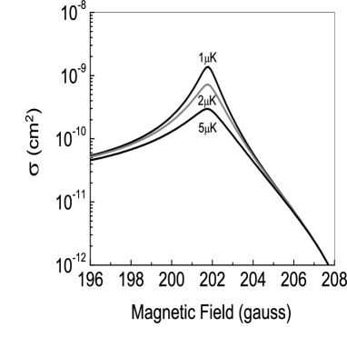
Figure 2: (a) Thermally averaged cross section for $|9/2,-7/2\rangle|9/2,-7/2\rangle|1,1\rangle$ collisions as a function of magnetic field. The striking features of this curve are the sudden rise and change in width as the temperature is increased. (b) Thermally averaged cross section for $|9/2,-9/2\rangle|9/2,-7/2\rangle|0,0\rangle$ collisions as a function of magnetic field. The temperature dependence is only evident at the peak where it washes out the maximum value.

Figure 2 shows the thermally averaged cross section for the $m_{l}=1$ p-wave resonance, Fig. 2 (a), and for the s-wave FR, Fig. 2 (b). The key features of Figure 2 (a) are the sudden rise of the cross section and thermal broadening, which grows dramatically at high field as the temperature increases. The rise comes from the sudden appearance of the the narrow resonance at positive collision energies as the magnetic field is tuned. This rise is not temperature dependent because, regardless of temperature, the threshold is first degenerate with the bound state at a unique magnetic field. By contrast, the high field tail of the resonance is sensitive to temperature because once the bound state has passed through threshold the energy dependent cross section peaks at higher energies for higher field values. For a fixed magnetic field the high field side of the FR, there is a well defined, narrow resonance at a particular energy (Fig. 1 (a)). If the temperature is low, very few atom pairs can access this resonance. At higher temperatures more atoms experience resonant scattering, increasing $\langle\sigma\rangle$.

This characteristic asymmetric profile is not present is s-wave FRs. The s-wave FR is shown in Fig. 2 (b) near its peak. The only effect of temperature in the elastic cross section is to wash out the peak of the resonance as the temperature is increased. This behavior follows from the relatively structureless energy-dependent cross section in Fig. 1 (b).

III The Doublet Feature

The valence electrons of ultra-cold alkali atoms interact via a magnetic dipole-dipole interaction of the form

$$H_{ss}=-\alpha^{2}{3({\bf\hat{R}}\cdot{\bf\hat{s}}_{1})({\bf\hat{R}}\cdot{\bf\hat{s}}_{2})-{\bf\hat{s}}_{1}\cdot{\bf\hat{s}}_{2}\over R^{3}}$$ (2)

where $\alpha$ is the fine structure constant, ${\bf\hat{s}}_{i}$ the spin of the valence electron on atom $i$, $R$ is the interatomic separation, and ${\bf\hat{R}}$ is the normal vector defining the interatomic axis. Another way of writing this interaction that isolates the spin and partial wave operators is

$$H_{ss}=-{\alpha^{2}\sqrt{6}\over R^{3}}\sum_{q=-2}^{2}(-1)^{q}C^{2}_{q}\cdot(s_{1}\otimes s_{2})^{2}_{-q}.$$ (3)

Here $C^{2}_{q}(\theta,\phi)$ is a reduced spherical harmonic that depends on the relative orientation of the atoms, and $(s_{1}\otimes s_{2})^{2}_{-q}$ is the second rank tensor formed from the rank-1 spin operators Brink . $C^{2}_{q}$ acts on the partial wave component of the quantum state, $|lm_{l}\rangle$, while the $s_{i}$’s in $(s_{1}\otimes s_{2})^{2}_{-q}$ act on the electronic spin state of the atoms. Equation (3) leads to an interplay of partial wave and spin, which contributes an orientation-dependent energy to the Hamiltonian. The matrix element of Eq. (3) in our present basis is Burke2

$$-{\alpha^{2}\sqrt{6}\over R^{3}}\sum_{q=-2}^{2}(-1)^{q}{\langle l^{\prime}m_{l}^{\prime}|C^{2}_{q}|lm_{l}\rangle}\times$$

$${\langle f_{1}^{\prime}m_{f_{1}}^{\prime}|\langle f_{2}^{\prime}m_{f_{2}}^{\prime}|(s_{1}\otimes s_{2})^{2}_{-q}|f_{1}m_{f_{1}}\rangle|f_{2}m_{f_{2}}\rangle}.$$ (4)

This term in the Hamiltonian couples different partial waves for $l^{\prime}=l\pm 2$, and it couples different partial wave projections $m_{l}$ for $l^{\prime}=l\pm 2$ and $l=l^{\prime}\neq 0$. For elastic s-wave scattering ($l=l^{\prime}=0$) equation (III) vanishes by symmetry. This term only plays a role in s-wave scattering for s$\rightarrow$d wave transitions. However for p-wave scattering ($l=l^{\prime}=1$) this interaction does not vanish, i.e. $\langle 1m_{l}^{\prime}|C_{q}^{2}|1m_{l}\rangle\neq 0$. Furthermore, for elastic scattering, $q=0$, the interaction depends on $m_{l}$, since $\langle 11|C_{0}^{2}|11\rangle=-{1\over 5}$ and $\langle 10|C_{0}^{2}|10\rangle={2\over 5}$. The fact that the dipole-dipole interaction does not contribute equally to all values of $m_{l}$ means that bound states with different $m_{l}$ have different energies. This implies that FRs with different values of $m_{l}$ couple to distinct bound states and thus have different magnetic field dependences.

The difference between the $m_{l}$ projections can be understood intuitively by considering the dipole-dipole interaction of the two atoms. For the $|9/2,-7/2\rangle$ spin states case the electronic spins are essentially aligned with the field. When two dipoles are aligned head to tail they are in an attractive configuration, corresponding to ${\bf\hat{R}}\cdot{\bf\hat{s}_{i}}=1$ in Eq. (2). Vice-versa when the dipoles are side by side they are in a repulsive configuration, ${\bf\hat{R}}\cdot{\bf\hat{s}_{i}}=0$.

Viewing the motion of the atoms in the resonant state as classical, circular orbits, the cases $m_{l}=0$ and $m_{l}=1$ are distinguished as in Figure 3. For $m_{l}=0$, in Fig. 3 (a), the motion of the atoms is in a plane containing the magnetic field. Classically this corresponds to motion described by the angle $\theta$, where the magnetic field lies in the $\hat{z}$ direction. The interaction for $m_{l}=0$ alternates between attractive and repulsive as the dipoles change between head to tail attraction and side by side repulsion. On the other hand, for $|m_{l}|=1$, shown in Fig. 3 (b), the motion of the atoms is in the plane perpendicular to the magnetic field. Classically this corresponds to motion described by the angle $\phi$. This interaction is only repulsive, because the dipoles are held in the side-by-side configuration. Since the dipole-dipole interaction for $|m_{l}|=1$ has only a repulsive influence it forms a resonant state with higher energy.

Figure 4 shows the total elastic cross section as a function of field at several temperatures. One can clearly see the doublet feature in the cross section at low temperature. The first peak corresponds to $|m_{l}|=1$. The doublet cannot be resolved at high temperature because the width of the resonance is wider than the splitting.

The energy shift can be estimated using perturbation theory. The energy shift due to the dipole-dipole interaction is given in perturbation theory as

$$\Delta E_{m_{l}=0}={-\alpha^{2}\surd 6}\langle 10|C_{0}^{2}|10\rangle\langle\Phi_{mol}|{(s_{1}\otimes s_{2})^{2}_{0}\over R^{3}}|\Phi_{mol}\rangle$$ (5)

$$\Delta E_{m_{l}=1}={-\alpha^{2}\surd 6}\langle 11|C_{0}^{2}|11\rangle\langle\Phi_{mol}|{(s_{1}\otimes s_{2})^{2}_{0}\over R^{3}}|\Phi_{mol}\rangle.$$ (6)

Here $|\Phi_{mol}\rangle$ is the full multi-channel molecular wave function without the magnetic dipole-dipole interaction. This is the molecular state that couples to the continuum creating the FR. We notice that the perturbation is the same for each component, except for the angular coefficients in Equations (5) and (6). When these equations are evaluated, we find that the energy difference in the molecules,$|\Delta E_{m_{l}=1}-\Delta E_{m_{l}=0}|$, is $3.7\mu$K, which is close to the closed coupling calculation result of $4.7\mu$K. As the bound states are brought through threshold, we find that their energy difference translates into a peak separation of $0.5$ G, determined from the closed coupling scattering calculations.

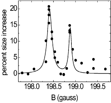
Figure 5: The p-wave FR observed through heating of the gas, clearly showing the doublet feature of the p-wave resonance. The cloud started at T=0.34 $\mu$K and then was held at a constant magnetic field. Inelastic processes at the FR, 3-body dominated, heat the cloud resulting in an increase in the measured size of the trapped cloud. The curve is only a guide to the eye.

Experimentally we have observed the doublet p-wave resonance in an ultra-cold gas of ⁴⁰K through inelastic collisional effects. A gas of atoms in the $|9/2,-7/2\rangle$ state of ⁴⁰K was prepared at T=0.34 $\mu$K in an optical dipole trap characterized by a radial frequency of $\nu_{r}$=430 Hz and an axial frequency of $\nu_{z}$=7 Hz Loftus ; Regal . The gas was then held at a magnetic field near resonance for 260 $\mu$s. The resulting Gaussian size of the trapped gas in the axial direction was measured as a function of magnetic field. The result of this measurement is shown in Fig. 5.

The observed heating of the gas in Figure 5 is due to inelastic processes that occur at the p-wave FR. The result clearly shows the predicted doublet structure. The splitting between the two peaks is measured to be 0.47$\pm$8 G, in good agreement with the theory. The dominant inelastic processes are 3-body losses Regal ; Esry , which lie at a slightly lower field than the elastic resonance peak Regal .

IV Effective Range Expansion of the p-wave FR

To compute many-body properties of degenerate gases the s-wave scattering length is often used to mimic the essential 2-body physics. Near a FR the scattering length diverges and can be represented well by $a=a_{bg}(1-{\Delta\over B-B_{0}})$ where $a_{bg}$ is the back ground scattering length, $\Delta$ is the width, $B_{0}$ is the location of the s-wave resonance. Scattering length is defined as $a=^{\lim}_{k\rightarrow 0}-\tan(\delta_{0})/k$ where $\delta_{0}$ is the s-wave phase shift and $k=\sqrt{2\mu E}$ where $\mu$ is the reduced mass.

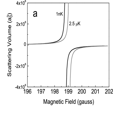
Figure 6: (a) The p-wave scattering volume for $|m_{l}|=1$ as a function of magnetic field at two different energies. Notice that both the location at which the scattering volume diverges and the width vary with collision energy. (b) $k^{3}\cot(\delta_{1})$ for the $|m_{l}|=1$ p-wave resonance as a function of energy for several different values of magnetic field.

For p-wave collisions the relevant quantity is the scattering volume, $v=^{\lim}_{k\rightarrow 0}-\tan(\delta_{1})/k^{3}$. A simple form like the one for $a$ is inadequate for parameterization of the p-wave scattering volume because the p-wave resonance has a complicated energy dependence. Fig. 6(a) shows the p-wave scattering volume as a function of field and energy. The curves show that as the energy is increased the location and width of the resonance change.

To adequately parameterize the p-wave phase shift across the resonance one must use the second order term in the the effective range expansion MM . Fig. 6(b) shows $k^{3}\cot(\delta_{1})$ plotted as a function of energy for several magnetic fields. This set of curves can then be fit using effective range expansion of the form

$$k^{3}\cot(\delta_{1})=-{1\over v}+{c}k^{2}.$$ (7)

Where $\delta_{1}$ is the p-wave phase shift, $v$ is the scattering volume, and $c$ the second coefficient in the expansion, analogous to the effective range in the s-wave expansion, but with units $a_{0}^{-1}$. Both $v$ and $c$ are functions of magnetic field. Fitting $v$ and $c$ to quadratic functions of $B$, which is adequate for the energy range of $E<10^{-6}$ K and magnetic field range of 195 to 205 gauss, we find

$${1\over v_{m_{l}=0}}=8.68155\times 10^{-5}-8.29778\times 10^{-7}B$$

$$+1.97732\times 10^{-9}B^{2}$$

$$c_{m_{l}=0}=-1.64805+0.01523B-3.54471\times 10^{-5}B^{2}$$

$${1\over v_{|m_{l}|=1}}=7.83424\times 10^{-5}-7.456621\times 10^{-7}B$$

$$+1.76807\times 10^{-9}B^{2}$$

$$c_{|m_{l}|=1}=-2.36792+0.02264B-5.45051\times 10^{-5}B^{2}$$

where B is magnetic field in gauss. These fits for $1\over v$ and $c$ accurately reproduce $k^{3}\cot(\delta_{1})$ to within $3\%$ on the interval specified. This fit does not include experimental uncertainties, rather the fit is designed to reproduce the the closed coupling calculation with the optimal scattering parameters.

V Implications for experiments

Because of the p-wave FR, angular dependence of scattering is under the experimenter’s control. For example if magnetic field tuned to 199.0 G in the ${}^{40}K$ p-wave FR the dominant interactions in the gas will be perpendicular to the field axis, which follows from the angular distribution corresponding to the spherical harmonic $Y_{11}(\theta,\phi)$ leading to enhanced collisions rates away from the field axis. Whereas if the field is tuned 0.5 G higher, at cold temperatures the interaction will be dominated by $Y_{10}(\theta,\phi)$, characterized by enhanced collisions along the field axis. The angular dependence of the collisions also has implications for the inelastic 2-body processes. These processes are characterized by two atoms gaining a predictable amount of energy governed by hyperfine splitting and are redistributed in a well defined angular manner.

P-wave FRs offer a means to experimentally study anisotropic interactions in systems other than identical fermions. For example, we predict that there are p-wave FRs in distinct spin states of bosonic ⁸⁵Rb and in the Bose-Fermi mixture of ⁸⁷Rb-⁴⁰K, shown in Table 1. The Rb calculations used potentials that are consistent with Ref. Roberts . The Rb-K calculations are consistent with Ref. Simoni . On resonance the p-wave cross section becomes comparable to the background s-wave scattering. This means that it could have an equally important role in determining the collisional behavior and mean-field interaction of a thermal gas or condensate.

VI Conclusion

We have presented characteristics of p-wave FRs. An interesting characteristic is the doublet feature for the FR with $l=1$. The splitting is caused by the dipole-dipole interaction having distinct values depending on partial wave projection. This might in turn offer a means to study anisotropic interactions in quantum gases. Another feature of the p-wave FR is the asymmetric thermal broadening, which arises from the resonant state moving away from threshold as the magnetic field is tuned. Generally, we expect the broadening to occur for fields which the $v<0$. Just as a p-wave FR splits into two components an $l$-wave FR will split into $l+1$ components.

Table 1: Predicted p-wave resonances in bosonic Rb and a Bose-Fermi mixture of Rb-K. The Rb p-wave FRs gain a bound state as the field is increased, whereas the opposite is true for ${}^{40}K$ p-wave FR. This is why in Rb the ${m_{l}=0}$ resonance is lower in field.

Species	Spin States	Magnetic Field
${}^{85}Rb$	$|2,-2\rangle|2,-1\rangle$	$B_{m_{l}=0}=247.3$	$\pm$ 5 G
		$B_{|m_{l}|=1}=248.0$	$\pm$ 5 G
${}^{85}Rb$ ${}^{87}Rb$	$|2,-2\rangle_{85}|1,-1\rangle_{87}$	$B_{m_{l}=0}=292.8$	$\pm$ 30 G
		$B_{|m_{l}|=1}=292.5$	$\pm$ 30 G
${}^{87}Rb$ ${}^{40}K$	$|1,1\rangle|9/2,-9/2\rangle$	$B_{m_{l}=0}=540.0$	$\pm$ 30 G
		$B_{|m_{l}|=1}=540.3$	$\pm$ 30 G

Figure 1: (a) P-wave elastic cross section versus energy for $|9/2,-7/2\rangle|9/2,-7/2\rangle|1,1\rangle$ collisions for different magnetic field values. For each curve the magnetic field in gauss is indicated. The lowest curve shows an off-resonance cross section. (b) For comparison, the s-wave elastic cross section versus energy for $|9/2,-9/2\rangle|9/2,-7/2\rangle|0,0\rangle$ collisions for different magnetic field values. The s-wave FR peaks at B=201.6 G. Compared to the p-wave FR these have little structure. The solid line is the unitarity limit.

Figure 3: Schematic representation of classical dipoles interacting in different circular orbits. Shown in (a) is an orbit with $m_{l}=0$, which is in a plane containing the magnetic field. Here the dipoles sometimes attract and sometimes repel. In (b) is shown an orbit with $|m_{l}|=1$, in a plane perpendicular to the magnetic field. Here the atoms predominately repel one another.

Figure 4: The thermally averaged elastic cross section for the p-wave FR, including all partial wave projections $m_{l}=-1,0,1$. At low temperatures, the doublet splitting emerges clearly, but it is washed out a higher temperatures due to thermal broadening. The lower field resonance has $|m_{l}|=1$ and the higher field resonance has $m_{l}=0$.

References

- (1) Quantum Physics Division, National Institute for Standards and Technology.
- (2) S. Inouye, M. R. Andrews, J. Stenger, H.J . Miesner, D. M. Stamper-Kurn, and W. Ketterle, Nature (London) 392, 151 (1998).
- (3) Ph. Courteille, R. S. Freeland, D. J. Heinzen, F.A. van Abeelen, and B. J. Verhaar, Phys. Rev. Lett. 81, 69 (1998).
- (4) J. L. Roberts, N. R. Claussen, J.P. Burke, C. H. Greene, E. A. Cornell, and C. E. Wieman Phys. Rev. Lett. 81, 5109 (1998).
- (5) V. Vuletić, A.J. Kerman, C. Chin, and S. Chu, Phys. Rev. Lett. 82, 1406 (1999).
- (6) A. Marte, et al., Phys. Rev. Lett. 89, 283202 (2002).
- (7) T. Loftus, C. A. Regal, C. Ticknor, J. L. Bohn and D. S. Jin, Phys. Rev. Lett. 88, 173201 (2002).
- (8) S. Jochim, M. Bartenstein, G. Hendl, J. Denschlag, R. Grimm, A. Mosk and M. Weidemüller Phys. Rev. Lett. 89, 273202 (2002).
- (9) K. M. O’Hara, S. L. Hemmer, S. R. Granade, M. E. Gehm, J. E. Thomas, V. Venturi, E. Tiesinga, and C.J. Williams, Phys. Rev. A. 66, 041401 (2002).
- (10) K. Dieckmann, C. A. Stan, S. Gupta, Z. Hadzibabic, C.H. Schunck, and W. Ketterle, Phys. Rev. Lett. 89, 203201 (2002).
- (11) C. A. Regal, C. Ticknor, J. L. Bohn, and D. S. Jin, Phys. Rev. Lett. 90, 053201 (2003).
- (12) H.T.C. Stoof, M. Houbiers, C. A. Sackett, and R.G. Hulet, Phys. Rev. Lett. 76, 10 (1996).
- (13) M. Holland, S.J.J.M.F. Kokkelmans, M.L. Chiofalo, and R. Walser, Phys. Rev. Lett. 87, 120406 (2001).
- (14) H. Suno, and B. D. Esry, C. H. Greene, Phys. Rev. Lett. 90, 53202 (2003).
- (15) C. A. Regal and D. S. Jin, Phys. Rev. Lett. 90, 230404 (2003).
- (16) T. Bourdel, et al., Phys. Rev. Lett. 91, 20402 (2003).
- (17) S. Gupta, et al., Science 300: 1723-1726;
- (18) C. A. Regal, C. Ticknor, J. L. Bohn, and D. S. Jin, Nature 424, 47 (2003).
- (19) K. E. Strecker, G. B. Partridge, R. G. Hulet. Phys. Rev. Lett. 91, 80406 (2003);
- (20) J. Cubizolles et al., cond-mat 030801 (2003);
- (21) S. Jochim, et al., cond-mat 0308095 (2003);
- (22) B. DeMarco, J. L. Bohn, J.P. Burke, Jr., M. Holland, and D. S. Jin, Phys. Rev. Lett. 82, 4208 (1999).
- (23) For a review see: M. Baranov, L. Dobrek, K. Goral, L. Santos, and M. Lewenstein, Physica Scripta, T 102, 74 (2002).
- (24) B.R. Johnson, J. Comp. Phys., 13, 445 (1973).
- (25) J. Burke, Ph.D. Thesis, University of Colorado (1999).
- (26) L. Li, A. M. Lyyra, W. T. Luh, and W. C. Stwalley, J. Chem. Phys. 93, 8452 (1990), W. T. Zemke,C. Tsai, and W. C. Stwalley, J. Chem. Phys. 101, 10382 (1994)
- (27) C. Amiot J. Mol. Spectroscopy 147, 370 (1991).
- (28) D. M. Brink and G. R. Satchler, Angular Momentum, Clardeon Press, Oxford ©1993.
- (29) N.F. Mott and H. S. W. Massey, The Theory of Atomic Collisions 3rd Ed., Clardeon Press, Oxford ©1965
- (30) J. L. Roberts, James P. Burke, Jr., N. R. Claussen, S. L. Cornish, E. A. Donley, and C. E. Wieman, Phys Rev. A 64, 24702 (2001).
- (31) A. Simoni, F. Ferlaino, G. Roati, G. Modugno, and M. Inguscio, Phys. Rev. Lett. 90, 163202 (2003).