Helical filaments with varying cross section radius

Abstract

The tridimensional configuration and the twist density of helical rods with varying cross section radius are studied within the framework of the Kirchhoff rod model. It is shown that the twist density increases when the cross section radius decreases. Some tridimensional configurations of helix-like rods are displayed showing the effects of the nonhomogeneity considered here. Since the helix-like solutions of the nonhomogeneous rods do not present constant curvature and torsion a set of differential equations for these quantities is presented. We discuss the results and possible consequences.

Helical filaments are tridimensional structures universally found in Nature. They can be seen in very small sized systems, as biomolecules tamar and bacterial fibers wolge , and in macroscopic ones, as ropes, strings, and climbing plants alain ; foot1 ; tyler . All these objects have in common the fact that the mathematical geometric properties of the 3D-space curve related to their axis, namely the curvature, $k_{F}$, and the torsion, $\tau_{F}$, are constant nize .

The so-called Kirchhoff rod model has been proved to be a good framework to study the statics nize ; vander and dynamics goriely of long, thin and inextensible elastic rods kirch ; dill . The applications of the Kirchhoff model range from Biology tamar ; col1 ; tyler to Engineering sun . In these cases, the rod or filament is considered as being homogeneous, but the case of nonhomogeneous rods have been also considered in the literature. It has been shown that nonhomogeneous Kirchhoff rods may present spatial chaos holmes ; davies and that helical transitions occur in the tridimensional configurations of rods with periodic variation of the Young’s modulus fonseca0 . A comparison between homogeneous and nonhomogeneous rods subject to given boundary conditions and mechanical parameters was performed by da Fonseca and de Aguiar in fonseca1 . The effects of a nonhomogeneous mass distribution in the dynamics of unstable closed rods have been analyzed by Fonseca and de Aguiar fonseca2 . Goriely and McMillen alain2 studied the dynamics of cracking whips whip and Kashimoto and Shiraishi moto studied twisting waves in inhomogeneous rods.

Here, using the Kirchhoff model, we shall present the results for the equilibrium solutions of nonhomogeneous rods with varying cross section radius and no intrinsic curvature. Only the solutions classified by Nizette and Goriely nize as being helical will be considered: the straight rod, the twisted planar ring and the helix. We shall show that the twist density varies along the rod inversely proportional to the fourth power of the radius of the cross section. Also, it will be seen that the curvature, $k_{F}$, and the torsion, $\tau_{F}$, are not constant for the helix-like solutions with nonhomogeneous cross section radius.

The motivations for this work are: i) the study of failure or rupture of cables azevedo ; sayed . For example, it was shown that shoreline anchor rods rupture at the region where the rod diameter diminishes due to corrosion sayed . The fact that, for twisted rods, the twist density increases in the regions where the rod diameter decreases can be related to the onset of the failure; ii) the shape of some climbing plants have filamentary helical structures (spring-like tendrils) whose radius and pitch are not constant alain . Such a tridimensional configuration, with the radius and the pitch varying along the rod, will be shown to be a possible solution of the Kirchhoff model for the nonhomogeneous rod. Other motivations are related to defects kronert , distortions geetha and the rule of twisting turner in biological molecules.

The static Kirchhoff equations, in scaled variables, for rods with circular cross section and no intrinsic curvature are given by:

$$\begin{array}[]{ll}\mathbf{F}^{\prime}=0\;,\\ \mathbf{M}^{\prime}+\mathbf{d}_{3}\times\mathbf{F}=0\;,\\ \mathbf{M}=I(s)\,k_{1}\,\mathbf{d}_{1}+I(s)\,k_{2}\,\mathbf{d}_{2}+\Gamma\,I(s)\,k_{3}\,\mathbf{d}_{3}\;,\end{array}$$ (1)

where $s$ is the arc-length of the rod, the prime ^′ denotes differentiation with respect to $s$ and the vectors $\mathbf{F}$ and $\mathbf{M}$ are the resultant force, and corresponding moment with respect to the axis of the rod, respectively, at each cross section. $\mathbf{d}_{i}$, $i=1,2,3$, compose the director basis with $\mathbf{d}_{3}$ chosen to be the vector tangent to the axis of the rod and $\mathbf{d}_{1}$ and $\mathbf{d}_{2}$ lie in the plane of the cross section. $k_{i}$ are the components of the twist vector, $\mathbf{k}$, that controls the variations of the director basis along the rod through the relation $\mathbf{d}^{\prime}_{i}=\mathbf{k}\times\mathbf{d}_{i}$. $k_{1}$ and $k_{2}$ are related to the curvature ($k_{F}=\sqrt{k^{2}_{1}+k^{2}_{2}}$) and $k_{3}$ is the twist density of the rod. $\Gamma=2\mu/E$ is the adimensional elastic parameter, with $\mu$ and $E$ being the shear and the Young’s moduli, respectively. $I(s)$ is the variable moment of inertia that is related to the radius of the cross section through the relation $I(s)=R^{4}(s)$ (valid in scaled units). Writing the resultant force $\mathbf{F}$ in the director basis, $\mathbf{F}=f_{1}\mathbf{d}_{1}+f_{2}\mathbf{d}_{2}+f_{3}\mathbf{d}_{3}$, the equations (1) give six differential equations for the components of the resultant force and twist vector:

$$f^{\prime}_{1}-f_{2}\,k_{3}+f_{3}\,k_{2}=0\;,$$ (2a)

$$f^{\prime}_{2}+f_{1}\,k_{3}-f_{3}\,k_{1}=0\;,$$ (2b)

$$f^{\prime}_{3}-f_{1}\,k_{2}+f_{2}\,k_{1}=0\;,$$ (2c)

$$(I(s)\,k_{1})^{\prime}+(\Gamma-1)\,I(s)\,k_{2}\,k_{3}-f_{2}=0\;,$$ (2d)

$$(I(s)\,k_{2})^{\prime}-(\Gamma-1)\,I(s)\,k_{1}\,k_{3}+f_{1}=0\;,$$ (2e)

$$(\Gamma\ I(s)\ k_{3})^{\prime}=0\;.$$ (2f)

Since $I(s)=R^{4}(s)$, the equation (2f) shows that the twist density $k_{3}$ is inversely proportional to $R^{4}(s)$. Therefore, $k_{3}$ is not constant for nonhomogeneous cases. On the other hand, the component $M_{3}=\Gamma\,I\,k_{3}$ of the moment in the director basis (also called torsional moment), is a constant along the rod.

In order to look for helical solutions of the eqs. (2) the components of the twist vector $\mathbf{k}$ are expressed as follows:

$$k_{1}=k_{F}\sin\xi\;,\;k_{2}=k_{F}\cos\xi\;,\;k_{3}=\xi^{\prime}+\tau_{F}\;,$$ (3)

where $k_{F}$ and $\tau_{F}$ are the curvature and torsion of the rod, respectively. In the homogeneous case $k_{F}$ and $\tau_{F}$ are constant, and $\xi=(k_{3}-\tau_{F})s$ nize .

We shall consider the following cases: the straight rod, the twisted planar ring and the general helix-like rod.

i) The straight rod: $k_{F}=\tau_{F}=0$.

From eq. (3), $k_{1}=k_{2}=0$ and from eqs. (2),

$$\begin{array}[]{ll}k_{3}(s)=\frac{\mbox{Constant}}{I(s)}=\frac{M_{3}}{\Gamma\,R^{4}(s)}\;,\\ f_{1}=f_{2}=0\;\mbox{and}\;f_{3}\equiv T=\mbox{Constant}\;.\end{array}$$ (4)

$T$ is the tension applied to the rod. Figure 1 shows the twist density $k_{3}(s)$ for a straight rod with the cross section radius varying as

$$R(s)=1+0.1\cos(0.3s)\;,$$ (5)

in scaled units. The mechanical parameters used to obtain the rod displayed in Figure 1 were $M_{3}=10^{-1}$ (scaled units) and $\Gamma=0.9$.

ii) The twisted planar ring: $k_{F}=$ Constant and $\tau_{F}=0$.

The components of the twist vector for the twisted planar ring are:

$$\begin{array}[]{ll}k_{1}=k_{F}\sin\xi\;,\;k_{2}=k_{F}\cos\xi\;,\;\xi^{\prime}=k_{3}=\frac{M_{3}}{\Gamma\,R^{4}(s)}\;.\end{array}$$ (6)

Substituting the eqs. (6) in eqs. (2) shows that the twisted planar ring is a possible equilibrium solution only if the cross section radius is of the form:

$$R(s)=(A_{0}\cos(k_{F}\,s)+B_{0}\sin(k_{F}\,s)+C_{I}/k_{F}^{2})^{\frac{1}{4}}\;,$$ (7)

where $A_{0}$, $B_{0}$ and $C_{I}$ are constants.

Remark: considering $\tau_{F}=0$ and assuming that $k_{F}$ is a function of $s$ (instead of being a constant) there exist no solutions for eqs. (2). So, the existence of planar solution requires $k_{F}=$ Constant.

iii) The general helix-like rod: $k_{F}=k_{F}(s)$ and $\tau_{F}=\tau_{F}(s)$.

In this case, the eqs. (3) become:

$$k_{1}=k_{F}(s)\sin\xi\;,\;k_{2}=k_{F}(s)\cos\xi\;,\;k_{3}=\xi^{\prime}+\tau_{F}(s)\;.$$ (8)

Substituting eq. (8) in eqs. (2), extracting $f_{1}$ and $f_{2}$ from eqs. (2e) and (2d), respectively, differentiating them with respect to $s$ and substituting in eqs. (2a) and (2b) gives a set of differential equations for $k_{F}(s)$, $\tau_{F}(s)$ and $f_{3}(s)$:

$$\begin{array}[]{ll}[(I(s)\,k_{F}(s))(\Gamma\,k_{3}(s)-\tau_{F}(s))]^{\prime}-(I(s)\,k_{F}(s))^{\prime}\,\tau_{F}(s)=0\;,\\ (I(s)\,k_{F}(s))^{\prime\prime}+I(s)\,k_{F}(s)\,\tau_{F}(s)(\Gamma\,k_{3}(s)-\tau_{F}(s))-f_{3}(s)\,k_{F}(s)=0\;,\\ (I(s)\,k_{F}(s))^{\prime}\,k_{F}(s)+f^{\prime}_{3}(s)=0\;.\end{array}$$ (9)

These differential equations are nonlinear and depend on $R(s)$ through $I(s)$.

Figure 2 shows a helix-like rod for the following linear variation of the radius of the cross section:

$$R(s)=1+0.0023\,s\;.$$ (10)

The mechanical parameters, in scaled units, are $M_{3}=0.05$, $\Gamma=0.9$, $k_{F}(0)=0.05$, $\tau_{F}(0)=0.24$ and $f_{3}(0)=0$.

In the figure 2 we display $k_{3}(s)$ (full line) and $0.1\,R(s)$ (dashed line). We can see that the radius and pitch of the helix-like tridimensional configuration displayed on the left of figure 2 are not constant.

Figure 3 shows the numerical solution for the curvature $k_{F}(s)$ (full line) and torsion $\tau_{F}(s)$ (dashed line) for the helix-like rod shown in the figure 2. Despite the simplicity of its tridimensional shape (figure 2, on the left) $k_{F}(s)$ and $\tau_{F}(s)$ are not simple functions of the arclength $s$, showing the nonlinear characteristic of the system.

Figure 4 shows an example of a helix-like rod with periodic variation of the radius of the cross section:

$$R(s)=1+0.1\sin(0.1\,s)\;.$$ (11)

The mechanical parameters, in scaled units, are $M_{3}=0.04$, $\Gamma=0.9$, $k_{F}(0)=0.19$, $\tau_{F}(0)=0.04$ and $f_{3}(0)=0.005$.

The functions $k_{3}(s)$ and $0.1\,R(s)$ are displayed in the figure 4 (full line and dashed line, respectively). In this case of periodic variation of the radius of the cross section, the tridimensional helix-like rod displayed in figure 4 (left) is more complicated than that displayed in the figure 2 (left).

Figure 5 shows the numerical solution for the curvature $k_{F}(s)$ (full line) and torsion $\tau_{F}(s)$ (dashed line) for the helix-like rod shown in the figure 4. The curvature and torsion are not simple functions of the arclength $s$ of the rod.

There is a kind of solution called free standing helix that is defined by setting the resultant force $\mathbf{F}=0$ tabor2 . In eqs. (9) $f_{3}(s)=0$ gives the following solution for the curvature and torsion of the rod:

$$\begin{array}[]{ll}(I(s)\,k_{F}(s))^{\prime}=0\;\Rightarrow\;k_{F}(s)=\frac{k_{F_{0}}}{I(s)}\;,\\ \tau_{F}(s)=\Gamma\,k_{3}(s)\;\Rightarrow\;\tau_{F}(s)=\frac{M_{3}}{I(s)}\;.\end{array}$$ (12)

Notice that for the free standing helix-like rod the curvature $k_{F}(s)$, and the torsion $\tau_{F}(s)$, will be analytical functions of the arclength $s$ if the moment of inertia $I(s)$ is given by an analytic function of $s$. Also $\frac{k_{F}(s)}{\tau_{F}(s)}$ is a constant for all $s$.

The variation of the twist density along the rod can be a key factor in a variety of phenomena. As mentioned before, the onset of a failure in a twisted cable can be related to the increasing of the twist density in a given region of the cable. In the Kirchhoff model, the torsional moment $M_{3}$ is constant along the rod. For a relatively high value of $M_{3}$ the twist density at a region of the rod with small diameter can be so large that it may not be valid the assumption of linear relationship between the torque and the components of the twist vector. Also, depending on how large the moment is, the behavior of the material could not be approximately elastic in the regions of small diameter. So, the increase of the twist density due to the decreasing diameter in a twisted rod may be the starting point of a process that can culminate with its rupture.

An interesting question arises for the important phenomenon known as writhing instability. In this phenomenon a local change in the twist can lead to a global reconfiguration of the rod that is a consequence of a topological constraint given by a mathematical theorem by White white . If the twist density varies along the rod, the question is to identify the region of the rod where this kind of instability will occur. The nonhomogeneity considered here can also have important consequences in the dynamics of this phenomenon golds . It will be a subject of a future publication.

Another implication of variable twist density along twisted rods is the problem of stability of equilibrium solutions. It is known that above a critical value of the twist density an equilibrium solution for the Kirchhoff model becomes unstable goriely ; tabor . Another good question is to investigate if a local increasing of the twist density above the critical value, can lead to a global instability of the related equilibrium solution. It could be important to the problem of failure mentioned before.

A very hard problem in differential geometry is obtaining a direct relationship between the curvature and the torsion with the radius and the pitch of a helix-like nonhomogeneous rod. Since the definitions of curvature and torsion involve the calculation of the modulus of the derivatives of tangent and normal vectors with respect to the arclength of the rod, for non constant radius and pitch, this relation is very complicated. The analysis of this problem will be considered in a future work.

It is interesting to note that the tridimensional configuration of the figure 2 displays a pattern in the radius and the pitch of the helix-like rod seen in the spring-like tendrils of some climbing plants. Since the young parts of the filament that composes the plant has smaller diameter than the older parts, these filaments are examples of rods with the nonhomogeneity considered here.

The numerical solutions obtained for $\tau_{F}(s)$ and the solutions for $k_{3}(s)$ of the helix-like cases show that the term $\xi^{\prime}$ of the equation (3) is not null as it was proved to be for the case of homogeneous helix tyler . It means that helix-like filaments formed by nonhomogeneous rods are not twistless.

The existence of intrinsic curvature may lead to other planar solutions. The helix-like solutions can also be influenced by the intrinsic curvature. This will be considered in a more complete work.

This work was partially supported by the Brazilian agencies FAPESP, CNPq and CAPES. The authors would like to thank Prof. Alain Goriely for suggesting the problem.

Figure 1: Top: a twisted straight rod with varying radius of the cross section. Bottom: the twist density $k_{3}$ as function of the arc-length $s$.

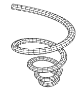
Figure 2: Left: helix-like rod having the radius of the cross section varying linearly with $s$ (eq. (10)). Right: $0.1\,R(s)$ (dashed line) and $k_{3}(s)$ (full line).

Figure 3: Geometric parameters: curvature, $k_{F}(s)$ (full line), and torsion, $\tau_{F}(s)$ (dashed line), for the equilibrium solution shown in the figure 2.

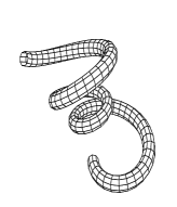
Figure 4: Left: helix-like rod having the radius of the cross section varying periodically with $s$ (eq. (11)). Right: $0.1\,R(s)$ (dashed line) and $k_{3}(s)$ (full line).

Figure 5: Geometric parameters: curvature, $k_{F}(s)$ (full line), and torsion, $\tau_{F}(s)$ (dashed line), for the equilibrium solution shown in the figure 4.

References

- (1) T. Schlick, Curr. Opin. Struct. Biol. 5, 245 (1995). W. K. Olson, Curr. Opin. Struct. Biol. 6, 242 (1996).
- (2) C. W. Wolgemuth, T. R. Powers and R. E. Goldstein, Phys. Rev. Lett. 84, 1623 (2000).
- (3) A. Goriely and M. Tabor, Phys. Rev. Lett. 80, 1564 (1998); Physicalia, 20, 299 (1998).
- (4) A set of interesting examples of the phenomenon of pervesion in helical filaments is provided by McMillen and Goriely tyler .
- (5) T. McMillen and A. Goriely, J. Nonlin. Sci. 12, 241 (2002).
- (6) M. Nizette and A. Goriely, J. Math. Phys. 40, 2830 (1999).
- (7) G. H. M. van der Heijden and J. M. T. Thompson, Nonlinear Dynamics 21, 71 (2000).
- (8) A. Goriely and M. Tabor, Nonlinear Dynamics 21, 101 (2000).
- (9) G. Kirchhoff, J. Reine Anglew. Math. 56, 285 (1859).
- (10) E. H. Dill, Arch. Hist. Exact. Sci. 44, 2 (1992); B. D. Coleman et al, Arch. Rational Mech. Anal. 121, 339 (1993).
- (11) I. Tobias, D. Swigon and B.D. Coleman, Phys. Rev. E 61, 747, (2000). B.D. Coleman, D. Swigon and I. Tobias, Phys. Rev. E 61, 759, (2000).
- (12) Y. Sun and J. W. Leonard, Ocean. Eng. 25, 443 (1997). O. Gottlieb and N. C. Perkins, ASME J. Appl. Mech. 66, 352 (1999).
- (13) A. Mielke and P. Holmes, Arch. Rat. Mech. 101, 319 (1988).
- (14) M. A. Davies and F. C. Moon, Chaos 3, 93 (1993).
- (15) A. F. da Fonseca, C. P. Malta and M. A. M. de Aguiar, “Helix-to-helix transitions in nonhomogeneous Kirchhoff filaments”, (to be published).
- (16) A. F. da Fonseca and M. A. M. de Aguiar, Physica D 181, 53 (2003).
- (17) A. F. Fonseca and M. A. M. de Aguiar, Phys. Rev. E 63, 016611 (2001).
- (18) A. Goriely and T. McMillen, Phys. Rev. Lett. 88, 244301 (2002).
- (19) A whip is a nonhomogenous thread with varying radius of cross section.
- (20) H. Kashimoto and A. Shiraishi, J. Sound and Vibration 178, 395 (1994).
- (21) C. R. F. Azevedo and T. Cescon, Eng. Failure Analysis 9, 645 (2002).
- (22) M. H. El-Sayed and B. Zaghloul, Materials Performance 40, 24 (2001).
- (23) W. A. Kronert et al, J. Mol. Biol. 249, 111 (1995).
- (24) V. Geetha, Int. J. Biol. Macromol. 19, 81 (1996).
- (25) M. S. Turner et al, Phys. Rev. Lett. 90, 128103 (2003).
- (26) A. Goriely and M. Tabor, Proc. Roy. Soc. London Ser. A 453, 2583 (1997).
- (27) J. H. White, Am. J. Math. 91, 693 (1969).
- (28) R. E. Goldstein, T. R. Powers and C. H. Wiggins, Phys. Rev. Lett. 80, 5232 (1998).
- (29) A. Goriely and M. Tabor, Phys. Rev. Lett. 77, 3537 (1996); Physica D 105 20 (1997).