The GNSS-R Eddy Experiment II: L-band and Optical Speculometry for Directional Sea-Roughness Retrieval from Low Altitude Aircraft

O. Germain, G. Ruffini, F. Soulat, M. Caparrini
Starlab, C. de l’Observatori Fabra s/n, 08035 Barcelona, Spain, http://starlab.es

B. Chapron
Ifremer, Technopole de Brest-Iroise BP 70, 29280 Plouzané, France, http://ifremer.fr

P. Silvestrin
ESA/ESTEC, Keplerlaan 1, 2200 Noordwijk, The Netherlands, http://esa.int

Abstract

We report on the retrieval of directional sea-roughness (the full directional mean square slope, including MSS, direction and isotropy) through inversion of Global Navigation Satellite System Reflections (GNSS-R) and SOlar REflectance Speculometry (SORES) data collected during an experimental flight at 1000 m. The emphasis is on the utilization of the entire Delay-Doppler Map (for GNSS-R) or Tilt Azimuth Map (for SORES) in order to infer these directional parameters. Obtained estimations are analyzed and compared to Jason-1 measurements and the ECMWF numerical weather model.
Keywords: GNSS-R, GPS, Galileo, Speculometry, SORES, sea roughness, Directional Mean Square Slope, Delay-Doppler Map.

1. Introduction

The use of Global Navigation Satellite System (GNSS) signals reflected by the sea surface as a remote sensing tool has generated considerable attention for over a decade [12, 13]. Among several applications, two classes have rapidly emerged in the community: sea-surface altimetry, which aims at retrieving the mean sea level like classical radar altimeters do, and sea-surface scatterometry or “speculometry” (see below for a justification of this neologism) for the determination of sea roughness and near surface wind. This paper addresses the latter application.

Inferring sea roughness from GNSS-R data requires (i) a parametric description of the sea surface, (ii) an electromagnetic model for sea-surface scattering at L-band and (iii) the choice of a GNSS-R data product to be inverted. In the literature, there is quite an agreement on the two first aspects. It has been recognized that the scattering of GNSS signals can be modeled as a Geometric Optics process (GO), where the fundamental physical process is the scattering from mirror-like surface elements. This is the reason why we use the term “speculometry”, from the latin word for mirror, speculo. Therefore, the most important feature of the sea surface is the statistics of facet slopes at about the same scale as the electromagnetic wavelength ($\lambda$). This is described by the bi-dimensional slope probability density function (PDF). Under a Gaussian assumption, three parameters suffice to fully define the sea-surface PDF: the directional mean square slope DMSS_λ, which results from the integration of the ocean energy spectrum at wavelengths larger than $\lambda$. The symbol DMSS_λ englobes the three parameters defining the ellipsoidal shape of the slope PDF: scale (total MSS), direction (Slope PDF azimuth) and isotropy (Slope PDF isotropy). The GNSS-R scattering model proposed by Zavorotny and Voronovich in [17] is based on GO, and is, to date, the reference model for the GNSS-R community. While for the purposes of specular scattering the sea-surface roughness is parametrized by the directional mean square slope in a direct manner, DMSS_λ is rarely emphasized as the geophysical parameter of interest. Instead, most authors prefer to link sea roughness to the near surface wind vector, which is thought to be more useful for oceanographic and meteorological users, but misleading. Indeed, this link requires an additional modeling layer and is an extra source of error. For instance, a wind-driven sea spectra is not suitable for inferring sea surface DMSS_λ when swell is present or the sea not fully developed. The connection between DMSS_λ and wind is thus modulated by other factors (e.g., swell, fetch and degree of maturity).

Usually, for technical reasons, the product inverted in GNSS-R speculometry is a simple Delay Waveform, that is, a 1D delay map of the reflected signal amplitude. Using a single GNSS emitter, the wind speed can be inferred assuming an isotropic slope PDF (i.e., the PDF’s shape is a circle) [8, 3, 11]. Attempts have also been made to measure the wind direction by fixing the PDF isotropy to some theoretical value (around 0.7) and using at least two satellites reflections with different azimuths [18, 9]. As investigated in the frame of the ESA OPPSCAT project (see [1] and [14]), it is nonetheless possible to work on a product of higher information content: the Delay-Doppler Map (DDM), a 2D delay-Doppler map of the reflected signal amplitude. The provision of an extra dimension opens the possibility to perform the full estimation of the DMSS_λ. In [7], Elfouhaily et al. developed a rapid but sub-optimal method based on the moments of the DDM to estimate the full DMSS_λ: this approach neglects the impact of the bistatic Woodward Ambiguity Function modulation of the Delay Doppler return.

The present paper was motivated by a recent experiment conducted by Starlab for the demonstration of GNSS-R altimetry. The altimetric aspects are reported elsewhere [15]. We note that the configuration of the flight was not optimized for speculometry: from 1000 m altitude, the sea-surface reflective area is essentially limited by the PRN C/A code, and the glistening zone is coarsely delay-Doppler mapped. In addition to the GNSS-R experiment, high resolution optical photographs of sun glitter were also taken, providing the SORES dataset (SOlar REflectance Speculometer). Since the classic study of Cox and Munk [4], it is well known that sea-surface DMSS_Opt can be inferred from such data. The availability of optical photographs thus provided us with an extra source of colocated information. Because there is a strong similarity between products —DDM for GNSS-R and the Tilt Azimuth Map (TAM) for SORES— and models —GO— the same inversion methodology can be applied to both datasets.

The goal of the paper is to investigate the full exploitation of the bidimensional GNSS-R DDM and SORES TAM products to infer the set of three DMSS_λ parameters. The driver of the study has been the exhaustive exploitation of the information contained in those 2D products. Consequently, the proposed approach relies on a least-square fit of speculometric models to datasets. We first describe in details the collected datasets and the associated pre-processing. Then, we present the speculometric models needed to infer data together with the inversion scheme. Finally, we provide the estimation results and discuss their coherence with other sources of data.

2. Dataset collection and pre-processing

The campaign took place Friday September 27th 2002 around 10:00 UTC, along the Catalan coast from Barcelona (Spain) up to the French border. An aircraft overflew the Jason-1 track 187 at 1000 m along 150 km and gathered 1.5 hours of GPS-R raw signals (see [16] for more details). Since it would have been computationaly too expensive to process the full track, it was divided into 46 10-second arcs (each spanning roughly 500 meters), sampled every 50 s (see Figure 1). The first arc started at GPS Second Of the Week 468008.63. The aircraft kinematic parameters were kept close to the nominal values specified in the mission plan: altitude=1000 m, speed=50 m/s and heading from North=30^o.

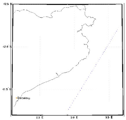
Figure 1: Map of the aircraft track divided into 46 10-second arcs.

We have selected three GPS satellites in optimal view during the experiment whose elevation and azimuth are given in Figure 2.

The raw GNSS-R data were recorded using the GPS reflection equipment provided by ESA. Specifically, the GPS direct and reflected signals were 1-bit sampled and stored a rate of 20.456 Mbit/s. The pre-processing step consisted in performing a delay-Doppler Pseudo Random Noise (PRN) code despreading to coherently detect the direct signal (from GPS emitter) and the reflected signal (scattered by sea-surface). We used the Starlab in-house software to produce three DDMs time-series (one per PRN), sampled into 46 arcs of 10 seconds each. The general processing strategy was to track the delay-Doppler of direct signal and then compute DDMs for both direct and reflected signals. These DDMs actually represent the filtered electromagnetic field of incoming signals, as processed with delay-Doppler value slightly different from those corresponding to the specular point. The coherent integration time was set to 20 ms to ensure a Doppler resolution of 50 Hz. The delay map spanned 80 correlation lags (i.e. +/- 1.95 $\mu$s) with a lag step of 48.9 ns, while the Doppler range spans -200 Hz to 200 Hz with a step of 20 Hz. Incoherent averaging was applied to each arc (the accumulation time was set to 10 s). This process aimed at reducing both thermal and speckle noise by a factor of $\sqrt{500}$. At the end, the GNSS-R product for one PRN and one arc was an average amplitude delay-Doppler map of size 81$\times$21.

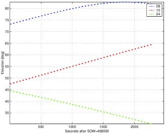
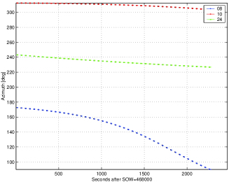
Figure 2: Elevation and Azimuth of three GPS satellites in view during the 46 10-second arcs.

The SORES photographs were taken from time to time along the track when the roll, pitch and yaw angles of the plane were negligible. The camera was a Leica dedicated to aerial photography. An inertial system (by Applanix) provided the time-tagged position for each snapshot. The film was a panchromatic Aviphot Pan 80. The focal length was 15.2 cm, and the photographic plate had an area of 23$\times$23 cm². The aperture angle was consequently 74.2^o. The observed area was a square with area 1.124$\times$1.124 km². The exposure time was fixed to 1/380 and aperture to f/4. The silver photographs were scanned and digital images were averaged to 400$\times$400 squared pixels, in order to be easily processed.

3. Models and inversion

3.1. Directional mean square slope

As discussed above, forward scattered signals at short wavelengths (optical but also L-band) are mostly sensitive to the specular scattering mechanism. Therefore, the strongest sea-surface signature in received signal is expected to be due to facet slope statistics at the relevant scales. The 2D slope probability density function (PDF) Gaussian model is given by

$${\cal P}(s)=\frac{e^{-\frac{1}{2}s^{{\dagger}}K^{-1}s}}{2\pi\sqrt{{\mbox{det}}(K)}},$$ (1)

where $s^{{\dagger}}=\left[\partial\zeta/\partial x\leavevmode\nobreak\ \leavevmode\nobreak\ \partial\zeta/\partial y\right]$ stands for the vector of directional slopes in some frame $xy$ and $K$ is the matrix of slope second order moments. The $xy$ frame mapped on sea-surface is defined as follows: it is centred on the specular point and has its $x$ axis aligned with the Transmitter-Receiver line. Mean-square slopes along major and minor principal axes are often referred to as MSS up-wind ($mss_{u}$) and MSS cross-wind ($mss_{c}$) respectively. The $K$ matrix is then obtained via a simple rotation,

$$K=R_{\psi}\cdot\left[\begin{array}[]{cc}mss_{u}&0\\ 0&mss_{c}\end{array}\right]\cdot R_{-\psi},$$ (2)

where $R_{\psi}$ is the usual rotation matrix of angle $\psi$, the angle between the $x$-axis and the slope principal axis.

Thus, $mss_{u}$, $mss_{c}$ and $\psi$ are the three geophysical parameters we wish to estimate. They can be thought of as the three parameters of an ellipse (see Figure 3) representing the slope PDF mapped on sea-surface. In the following, we will consider the equivalent set of parameters:

• Total MSS, defined as: $2\sqrt{mss_{u}.mss_{c}}$. This magnitude is actually proportional to ellipse area and can be interpreted in terms of wind speed, based on a particular wind-driven sea-surface spectrum like the Elfouhaily’s spectrum [6].

• Slope PDF azimuth (SPA), defined as the direction of semi-major axis with respect toNorth. As shown by Figure 3, this angle is $\pi+\Phi-\psi$, if $\Phi$ i s the satellite azimuth from North.

• Slope PDF isotropy (SPI), defined as $mss_{c}/mss_{u}$. When SPI=1, the slope PDF is isotropic and the glistening zone is circular. Low values of SPI indicate a highly directive PDF. Typically, SPI is expected to be around 0.65 for well developed sea-surface.

Figure 3: Sketch of the slope PDF and related frames.

3.2. GNSS-R speculometric model

The classical GNSS-R bistatic radar equation [17] links the average GNSS-R power return to sea-surface slope PDF. Processing the raw signal with various delay-Doppler values $(\tau,f)$, a DDM is computed whose theoretical expression is:

$$P(\tau,f) = \int dxdy\,\frac{G_{r}}{R_{t}^{2}R_{r}^{2}}\cdot\sigma^{0}\cdot$$ (3)

$$\chi^{2}\left(\tau_{m}-\tau_{c}-\tau,f_{m}-f_{c}-f\right)$$

where $G_{r}$ is the receiver antenna pattern, $R_{t}$ and $R_{r}$ are the distances from generic point on sea-surface to transmitter and receiver, $\sigma^{0}$ is the reflectivity, $\chi$ is the Woodward Ambiguity Function (WAF, see [13]), $\tau_{m}(x,y)$ and $f_{m}(x,y)$ are the delay-Doppler mapping on sea-surface and $\tau_{c}$ and $f_{c}$ are delay-Doppler centers. To first order, the reflectivity is proportional to the slope PDF:

$$\sigma^{0}=\pi|{\cal{R}}|^{2}\frac{q^{4}}{q_{z}^{4}}\leavevmode\nobreak\ {\cal P}\left(\frac{-q_{x}}{q_{z}},\frac{-q_{y}}{q_{z}}\right),$$ (4)

where $(q_{x},q_{y},q_{z})$ is the scattering vector and $|{\cal{R}}|^{2}=0.65$ is the specular Fresnel coefficient.

The presence of thermal noise biases the value of average power return. Hence, the average amplitude of the DDM can by modeled by

$$A(\tau,f)=\sqrt{\alpha.P(\tau,f)+b},$$ (5)

where $b$ stands for the bias in power. In particular, this effect is visible in the early-delay domain of the DDM: for delays lower than one-chip, the DDM amplitude has a no null value, often called ”grass level”. As we do not have a calibrated model an overall scaling parameter $\alpha$ is also needed in the model.

To sum up, the model features three parameters of interest and four “nuisance parameters”:

• the DMSS_λ, characterizing the Gaussian slope PDF: total MSS, isotropy (SPI) and azimuth (SPA),

• the DDM delay-Doppler centers: $\tau_{c}$ and $f_{c}$,

• overall scaling parameter: $\alpha$,

• grass level: $b$.

Other parameters required to run the forward model are recalled in Table 1.

Geometry	Aircraft: Altitude, speed and heading provided at 1 Hz Satellite: Elevation and azimuth provided at 1 Hz
Instrument	Antenna Pattern: measured in anechoic chamber Band: GPS L1 (19 cm) GPS Code: C/A
Processing	Integration Time: 20 ms Accumulation Time: 10 s Doppler span: [ -200 Hz , 200 Hz ], 20 Hz step Delay span: [-40 samples, 40 samples], 1 sample step

Table 1: Overview of the parameters necessary for running the DDM forward model.

3.3. SORES speculometric model

To date, results derived from the glitter-pattern of reflected sunlight as photographed by Cox and Munk in 1951 remain the most reliable direct measurements of wind-dependent slope statistics. As explained in their well-documented report [5], the sea-surface can be gridded with a Tilt ($\beta$) Azimuth ($\alpha$) Mapping of the small facet slopes. These are just a polar parametrization of the ($s_{x}$,$s_{y}$) slopes discussed in the previous section:

$$\left\{\begin{array}[]{ccc}s_{x}&=&\cos\alpha\cdot\tan\beta,\\ s_{y}&=&\sin\alpha\cdot\tan\beta.\end{array}\right.$$ (6)

The link between the small facet slope PDF ${\cal P}$ and the intensity in the photograh $I_{m}$ is given by

$$I_{m}(\alpha,\beta) = A_{0}\cdot{\cal P}(\alpha,\beta)\cdot f(\alpha,\beta,\phi)$$ (7)

$$+K\cdot I_{b}(\alpha,\beta),$$

where $I_{b}(\alpha,\beta)$ is the intensity of the picture background (i.e. far from the sun glint), $K$ and $A_{0}$ are multiplicative constants and $f$ is a transfer function,

$$f(\alpha,\beta,\phi)={\rho(1-\rho)^{3}\sin\phi\cos^{3}\mu\over\cos^{3}\beta\cos\omega},$$ (8)

with $\phi$: sun elevation, $\rho$: coefficient of reflection and $\mu$, $\omega$: two angles shown on Figure 4.

Figure 4: Geometry of the SORES experiment.

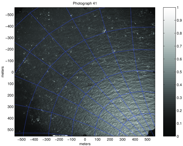
Figure 5: Tilt Azimuth Mapping overlaid on a SORES photograph.

The pixel intensity on the image comes principally from the additive contribution of sunglint and reflected skylight. The sunlight scattered by particles beneath the sea surface is assumed negligible and is not considered here. A model has been developed to remove reflections of sky radiance from the glint. The approach consists in considering each sea surface facet specular because, for a given location of the receiver, there always exists a “source” in the sky satisfying the specular reflection condition. Let’s consider the cell $(\alpha_{i},\beta_{i})$ of the TAM. It corresponds to the slope components required to reflect the solar rays onto the camera. The radiance of the sea surface due to reflected skylight in the cell $(\alpha_{i},\beta_{i})$ can thus be simply modeled by the integration of intensity over all the azimuths $\alpha$ and tilts $\beta$ except the azimuth $\alpha_{i}$ and the tilt $\beta_{i}$ of the corresponding cell.

3.4. Inversion scheme

Inversion was performed through a minimization of the root mean square difference between model and data products (i.e., DDMs for GNSS-R and TAMs for SORES). Numerical optimization was carried out with a steepest-slope-descent algorithm (Levenberg-Marquardt type adjustment). The three DMSS_λ as well as nuisance parameters ($\tau_{c}$, $f_{c}$ and $\alpha$ for the DDMs and $A_{0}$ and $K$ for the TAMs) were jointly estimated in an iterative manner: nuisance parameters (as a first step) and DMSS_λ (as a second step) were successively optimized, repeating this two-step sequence until convergence. Figure 6 gives qualitative examples of fit results for DDM and TAM.

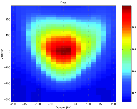
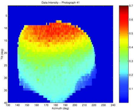
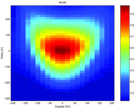
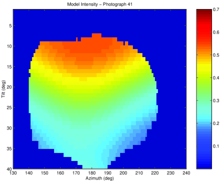
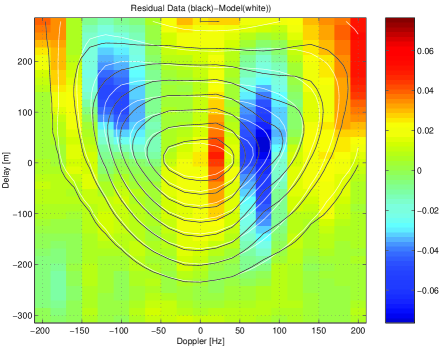
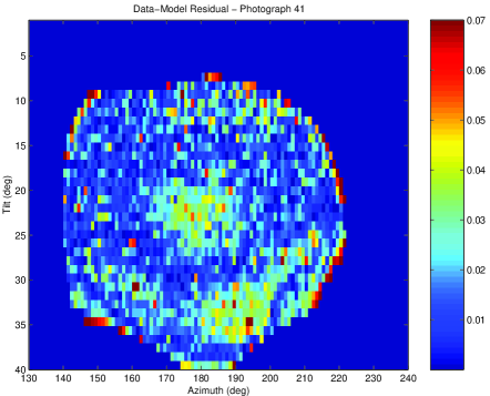
Figure 6: Examples of data products and their best-fit models. First column: GNSS-R Delay-Doppler Map (PRN08, arc 01). Second column: SORES Tilt-Azimuth Map (photograph 41). First row : Data. Second row : Best-fit Model. Third row : Data-Model Residual.

4. Results and discussion

Figure 7 shows total MSS, Slope PDF Azimuth and Slope PDF Isotropy along the aircraft track between latitudes 41.2^o and 42.2^o, as estimated by SORES and GNSS-R. Other sources of information are also shown for comparison:

• total MSS for C- and Ku- bands, derived from the Jason-1 $\sigma^{o}$ measurements at 1 Hz sampling (7 km) and 20 km resolution,

• wind direction provided by the ECMWF numerical weather model, with accuracy of 20^o, and

• swell direction derived from a spectral analysis of SORES images (the periodic pattern of long waves is indeed clearly observed on the photographs).

4.1. Total MSS

The total MSS has been plotted in log-scale in order to compare different frequency measurements more easily. The common trend for all bands is the increase of slope variance with latitude until a relative plateau is reached. Measurements of PRN08 and 24 show good agreement while PRN10 seems to be somewhat up-shifted. As expected, we observe that the level and dynamic of MSS decrease with longer wavelength: Optical, Ku, C and L band, in this order. Nevertheless, the level and dynamic range of GNSS-R plots (especially PRN10) seem a bit large for L-band measurements, when compared to C-band. Note however that Jason-1’s MSS have been obtained through the relationship $MSS=\kappa/\sigma^{o}$, $\kappa$ being an empirical parameter accounting for calibration offsets. Unfortunately, the uncertainty on $\kappa$ makes the absolute levels of Jason-1’s plots very doubtful. Here, as an illustration purpose, we have set $\kappa$=0.45 and $\kappa$=0.95 for C- and Ku-band respectively.

4.2. Slope PDF Azimuth

Using a single DDM, the estimation of SPA is degenerate in two particular cases: when the transmitter is at zenith or when the receiver moves torwards the transmitter [2]. In these two cases, the Delay-Doppler lines that map the glistening zone are symmetric around the receiver direction. Hence, one cannot distinguish between a slope PDF and its mirror image about the receiver direction. Here, PRN08 has its elevation comprised between 74 and 83 degrees. It is then very likely that the SPA estimated for this PRN is degenerate. For this reason, we have added on the plot the mirror image of the SPA about the receiver direction (30^o). We also note that the azimuth of PRN10 decreases down to 230^o at the end of the track, quite close from 210^o, the complementary of the receiver’s direction.

According to ECMWF data and SORES spectral analysis, wind and swell were slightly misaligned. PRN08 (or its mirror image) matches very well the swell direction and so does PRN10 along most of the track. This result underlines the fact that GNSS-R is not sensitive to wind only and that swell has a strong impact too. PRN24 has a different behaviour, in line with SORES. These two measurements agree relatively better with wind direction, although a discrepancy of 30^o is observed at the beginning of the track.

4.3. Slope PDF Isotropy

It is worth remembering that Elfouhaily’s wind-driven spectrum predicts a SPI value of 0.65, hardly sensitive to wind speed. Here we note that SPI varies quite significantly along the track for both GNSS-R and SORES. The important departure observed from the 0.65 nominal value is probably a signature of an under-developed sea and the presence of strong swell. Further research should be undertaken in order to better understand the potential information contained in this product.

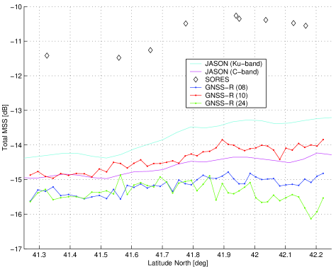
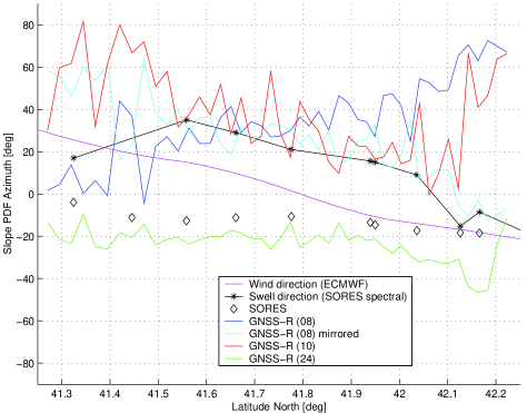
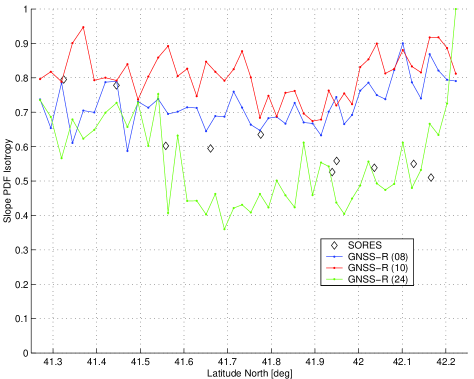
Figure 7: DMSS_λ estimated along the aircraft track. First row: Total MSS (in dB). Second row: Slope PDF Azimuth. Third row: Slope PDF Isotropy.

4.4. Link to wind speed

On Figure 8, we have plotted the estimated total MSS versus Jason-1’s wind speed together with two models:

• Elfouhaily’s sea-height spectrum, integrated for different cut-off wavelengths, and

• an empirical model proposed by Katzberg for L-band, based on a modification of Cox and Munk’s relationship: MSS=$0.9.10^{-3}\sqrt{9.48U+6.07U^{2}}$, $U$ being wind speed (private communication with J.L. Garrison, Purdue University).

We see that both SORES and GNSS-R estimations follow Elfouhaily’s model trend (MSS obtained by integrating the spectrum with the usual cut-off of 3 times the wavelength) but give higher values of MSS (from to 20 to 40% up-shifted). Actually, we have found that MSS estimates of PRN08 and 24 are very well fitted by Elfouhaily’s spectrum with a cut-off of one wavelength only. The 20% discrepancy can be explained by a strong sea state with a SWH twice as high as the one observed during the Cox and Munk’s experiment (almost 2 m compared to 1 m). At any rate, these results indicate that the wind-MSS link is not straightforward and that the DMSS_λ should be considered as a self-standing product for oceanographic users.

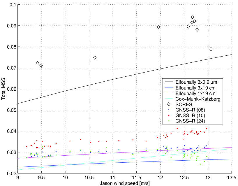
Figure 8: Total MSS versus Jason-1’s wind speed.

5. Conclusion

We have reported the first inversion of GNSS-R full Delay-Doppler Maps for the retrieval of the sea-surface directional mean square slope, DMSS_L. In addition, we have presented a repetition of the Cox and Munk experiment for DMSS_Opt retrieval through inversion of Tilt Azimuth Map of sun glitter optical photographs.

Our results show that both optical and L-band total MSS are 20% higher than predicted using Elfouhaily’s model for the observed wind speed (9 to 13 m/s). The SPA estimated by GNSS-R matches the swell direction with good accuracy for at least 2 out of 3 PRNs. A new geophysical product has been discussed: the slope PDF isotropy, which can be related to wind/wave misalignement as well the degree of sea development.

The analysis highlighted the important impact of sea-state unmodeled parameters (such as swell) in addition to wind stress on the measured DMSS_λ. Since speculometry is sensitive to slope processes over a wide range of scales, the link between DMSS_λ and wind is not straightforward: total MSS and SPA are definitely affected by swell. Quantitatively, the 20 % bias observed in SORES results can be explained by the impact of swell on the elevation spectrum. Consequently, DMSS_λ can and should be studied as an independent parameter, of independent geophysical value. We note however that the use of several wavelenghts could in principle be used to invert for all the parameters modulating the elevation spectrum, a line of future work.

Let us finally emphasize that the flight was not optimized for speculometry (1000 m altitude, 50 m/s speed) and that higher/faster flights are needed in the future in order to consolidate the concept of DDM inversion for DMSS_λ estimation.

References

- [1] GNSS-OPPSCAT, Utilization of scatterometry using sources of opportunity. Technical Report ESA-Contract 13461/99/NL/GD, 2000.
- [2] E. Cardellach and G. Ruffini. End to end performance. Technical report, 2000. WP3400 of OPPSCAT 1 Project - ESA Contract 13461/99/NL/GD.
- [3] E. Cardellach, G. Ruffini, D. Pino, A. Rius, A. Komjathy, and J. Garrison. Mediterranean balloon experiment: GPS reflection for wind speed retrieval from the stratosphere. To appear in Remote Sensing of Environment, 2003.
- [4] C. Cox and W. Munk. Measurement of the roughness of the sea surface from photographs of the sun’s glitter. Journal of the Optical Society of America, 44:838–850, 1954.
- [5] C. Cox and W. Munk. Slopes of the sea surface deduced from photographs of sun glitter. Bull. Scripps Inst. Ocean., 6:401–488, 1956.
- [6] T. Elfouhaily, B. Chapron, K. Katsaros, and D. Vandemark. A unified directional spectrum for long and short wind-driven waves. Journal of Geophysical Research, 102(15):781–796, 1997.
- [7] T. Elfouhaily, D.Thompson, and L. Linstrom. Delay-Doppler analysis of bistatically reflected signals from the ocean surface: Theory and application. IEEE Transactions on Geoscience and Remote Sensing, 40(3), 2002.
- [8] J.L. Garrison. Wind speed measurement using forward scattered GPS signals. IEEE Trans. Geoscience and Remote Sensing, 40:50–65, 2002.
- [9] J.L. Garrison. Anisotropy in reflected GPS measurements of ocean winds. In Proc. IEEE IGARSS, Toulouse, France, 2003.
- [10] J. Gourrion, D. Vandemark, S. Bailey, B. Chapron, C. Gommenginger, P.G. Challenor, and M.A. Srokosz. A two parameter wind speed algorithm for Ku-band altimeters. J. Atmos. Oceanic Tech., 19:2030–2048, 2002.
- [11] A. Komjathy, V.U. Zavorotny, P. Axelrad, G.H Born, and J.L. Garrison. GPS signal scattering from sea surface: Wind speed retrieval using experimental data and theoretical model. Remote Sensing of Environment, 73:162–174, 2000.
- [12] M. Martin-Neira. A PAssive Reflectometry and Interferometry System (PARIS): application to ocean altimetry. ESA Journal, 17:331–355, 1993.
- [13] G. Ruffini, M. Caparrini, O. Germain, F. Soulat, and J. Lutsko. Remote sensing of the ocean by bistatic radar observations: a review. Technical report, PARIS Beta WP1000 - ESA ESTEC Contract No. 15083/01/NL/MM, 2001. Available online at http://starlab.es.
- [14] G. Ruffini, J.L. Garrison, E. Cardellach, A. Rius, M. Armatys, and D. Masters. Inversion of GPS-R delay-Doppler mapping waveforms for wind retrieval. In Proc. IEEE IGARSS, Honolulu, HA, 2000.
- [15] G. Ruffini, F. Soulat, M. Caparrini, and O. Germain. The GNSS-R Eddy Experiment I: altimetry from low altitude aircraft. In Proceedings of the 2003 Workshop on Oceanography with GNSS-R. Starlab, July 2003.
- [16] F. Soulat. Sea surface remote-sensing with GNSS and sunlight reflections. Doctoral Thesis, Universitat Politècnica de Catalunya/Starlab, 2003.
- [17] V. Zavorotny and A. Voronovich. Scattering of GPS signals from the ocean with wind remote sensing application. IEEE Trans. Geoscience and Remote Sensing, 38(2):951–964, 2000.
- [18] C. Zuffada and T. Elfouhaily. Determining wind speed and direction with ocean reflected GPS signals. In Proceedings of Sixth Int. Conf. on Remote Sensing for Marine and Coastal Environments, Charleston, 2000.