Physics of Skiing:
The Ideal–Carving Equation and Its Applications

Abstract

Ideal carving occurs when a snowboarder or skier, equipped with a snowboard or carving skis, describes a perfect carved turn in which the edges of the ski alone, not the ski surface, describe the trajectory followed by the skier, without any slipping or skidding. In this article, we derive the “ideal-carving” equation which describes the physics of a carved turn under ideal conditions. The laws of Newtonian classical mechanics are applied. The parameters of the ideal-carving equation are the inclination of the ski slope, the acceleration of gravity, and the sidecut radius of the ski. The variables of the ideal-carving equation are the velocity of the skier, the angle between the trajectory of the skier and the horizontal, and the instantaneous curvature radius of the skier’s trajectory. Relations between the slope inclination and the velocity range suited for nearly ideal carving are discussed, as well as implications for the design of carving skis and snowboards.
Keywords: Physics of sports, Newtonian mechanics
PACS numbers: 01.80.+b, 45.20.Dd

1 Introduction

The physics of skiing has recently been described in a rather comprehensive book [1] which also contains further references of interest. The current article is devoted to a discussion of the forces acting on a skier or snowboarder, and to the derivation of an equation which describes “ideal carving”, including applications of this concept in practice and possible speculative implications for the design of technically advanced skis and snowboards. In a carved turn, it is the bent, curved edge of the ski or snowboard which forms some sort of “railroad track” along which the trajectory of the curve is being followed, as opposed to more traditional curves which are triggered by deliberate slippage of the bottom surface of the ski relative to the snow.

The edges of traditional skis have a nearly straight-line geometry. By contrast, carving skis (see figure 1) have a manifestly nonvanishing sidecut. Typical carving skis have a sidecut radius of the order of $16\,{\rm m}$ at a chord length of $170\,{\rm cm}$. However, parameters used in various models may be adapted to the intended application: e.g., models designed for less narrow curves may have a sidecut radius $R_{\rm SC}$ of about $19.5\,{\rm m}$ at a length of $180\,{\rm cm}$. Skis suited for very narrow slalom curves have an $R_{\rm SC}$ of about $14.5\,{\rm m}$ at a length of up to $164\,{\rm cm}$. A typical version suited for off-piste freestyle skiing features a typical length of $185\,{\rm cm}$ at a sidecut radius of $25.3\,{\rm m}$.

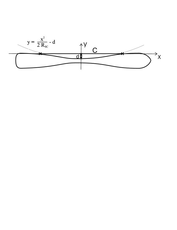
Figure 1: Overhead view on a typical carving ski. The tip of the ski points to the right. The geometry of the carving equipment involves the contact length $C$, the sidecut $d$ as well as the sidecut radius $R_{\rm SC}$. For a more traditional ski, the sidecut would be negligibly small, resulting in a very large sidecut radius.

The sidecut has been introduced first into the world of snow-related leisure activity by the snowboard where the wider profile of the instrument allowed for a realization of a rather marked sidecut without stringent demands on the materials used. The carved turn is the preferred turning procedure on a snowboard. Skidding should be avoided in competitions as far as possible because it necessarily entails frictional losses. In practical situations, carving skiers and snowboarders may realize astonishingly high tilt angles $\phi$ in the range of $[60^{o},80^{o}]$ (the “tilt angle” is the angle of line joining the board and the center-of-mass of the skier or boarder with the normal to the surface of the ski slope). In snowboarding, the transition from a right to a left turn is then often executed by jumping, with the idea of “glueing together” the trajectories of two perfect carved turns, again avoiding frictional losses. The sidecut radius $R_{\rm SC}$ of a snowboard may assume values as low as 6–8$\,{\rm m}$ at a typical chord length between $150\,{\rm cm}$ and $160\,{\rm cm}$.

This paper is organized as follows: In section 2, we proceed towards the derivation of the “ideal-carving equation”, which involves rather elementary considerations that we chose to present in some detail. The geometry of sidecut radius is discussed in section 2.1, and we then proceed from the simplest case of the forces acting along a trajectory perpendicular to the fall line (section 2.2) to more general situations (section 2.3). The projection of the forces in directions parallel and perpendicular to the skier’s trajectory lead to the concept of “effective weight” (section 2.4). The inclusion of a centrifugal force acting in a curve allows us to generalize this concept (section 2.5). In section 3, we discuss the “ideal-carving equation”, including applications. The actual derivation of the “ideal-carving equation” in section 3.1 is an easy exercise, in view of the preparations made in section 2. An alternative form of this equation has already appeared in [1]; in the current article we try to reformulate the equation in a form which we believe is more suitable for practical applications. The consequences which follow from the “ideal-carving equation” are discussed in section 3.2. Finally, we mention some implications for the design of skis and boards in section 4.

2 Toward the Ideal–Carving Equation

2.1 The Sidecut–Radius

According to figure 1, an approximate formula for the smooth curve described by the edge of the ski is $y\approx x^{2}/(2R_{\rm SC})-d$. This relation implies $d\approx C^{2}/(8R_{\rm SC})$. Therefore, we approximately have

$$\frac{{\rm d}^{2}y}{{\rm d}x^{2}}\,\approx\,\frac{1}{R_{\rm SC}}\,,$$ (1)

where $R_{\rm SC}$ is the sidecut radius of the ski. We then have

$$y\,\approx\,\frac{x^{2}}{2\,R_{\rm SC}}-d$$ (2)

along the edge of the ski. For $x=C/2$ we have $y\approx 0$ and therefore

$$d\approx\frac{C^{2}}{8\,R_{\rm SC}}\,,\qquad R_{\rm SC}\approx\frac{C^{2}}{8\,d}\,.$$ (3)

A typical carving ski with a chord length of $160\,{\rm cm}$ may have a sidecut radius as low as $R_{\rm SC}=14\,{\rm m}$. Estimating the contact length to be about $80\,\%$ of the chord length, we arrive at $d\approx~{}1.8\,{\rm cm}$. The maximum width of a ski (at the end of the contact curve) is of the order of $10\,{\rm cm}$, so that a sidecut of about $1.8\,{\rm cm}$ will lead to a minimum width which is roughly two thirds of the maximum width, leading to high structural demands on the material.

A typical snowboard has a length of about $168\,{\rm cm}$ and a width of about $25\,{\rm cm}$. The contact length is $125\,{\rm cm}$ in a typical case. A sidecut of

$$d\,\approx\,\frac{C^{2}}{8\,R_{\rm SC}}\approx\,2.4\,{\rm cm}$$ (4)

results, which means that for a typical snowboard, the relative difference of the minimum width to the maximum width is only $20\,\%$.

As the ski describes a carved turn, the radius of curvature $R$ along the trajectory varies with the angle of inclination $\phi$ of the normal to the ski slope with the normal to the ski surface. For $\phi\approx 0$, we of course have $R\approx R_{\rm SC}$. An elementary geometrical consideration shows that the effective sidecut $d^{\prime}$ at inclination $\phi$ is given by

$$d^{\prime}=\frac{d}{\cos\phi}\,.$$ (5)

The inclination-dependent sidecut-radius is therefore

$$R(\phi)=\frac{C^{2}}{8d^{\prime}}=R_{\rm SC}\,\cos\phi\leq R_{\rm SC}\,.$$ (6)

2.2 Trajectory Perpendicular to the Fall Line

The angle of inclination of the ski slope against the horizontal is $\alpha\in[0^{o},90^{o}]$. We assume the skier’s trajectory to be exactly horizontal. The work done by the gravitational force vanishes, and the skier, under ideal conditions, neither decelerates nor accelerates.

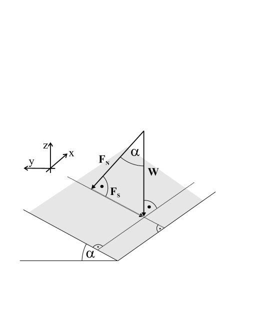
Figure 2: The skiing trajectory is indicated as parallel to a horizontal that lies in the plane described by the ski slope. That plane, in turn, is inclined against the horizontal by an angle $\alpha$. Of course, the angle $\alpha$ is equal to the angle of $\bm{F}_{\rm N}$ with $\bm{W}$. The force exerted on the skier in the gravitational field of the Earth is $\bm{W}$. It may be decomposed into a component $\bm{F}_{\rm N}$ perpendicular to the plane described by the ski slope, and a component $\bm{F}_{\rm S}$ lying in the plane of the slope.

With axes as outlined in figure 2, we have

$$\bm{W}=\left(\begin{array}[]{c}0\\ 0\\ -\,m\,g\end{array}\right)\,,\qquad\|\bm{W}\|=m\,g\,.$$ (7)

In order to calculate $\bm{F}_{\rm N}$, we project $\bm{W}$ onto the unit normal of the ski slope,

$$\hat{\bm{n}}=-\frac{\bm{F}_{\rm N}}{\|\bm{F}_{\rm N}\|}=\left(\begin{array}[]{c}0\\ -\sin\alpha\\ \cos\alpha\end{array}\right)\,,\qquad\bm{F}_{\rm N}=(\hat{\bm{n}}\cdot\bm{W})\,\hat{\bm{n}}\,.$$ (8)

This leads to the following representation,

$$\bm{F}_{\rm N}=m\,g\,\left(\begin{array}[]{c}0\\ \sin\alpha\,\cos\alpha\\ -\cos^{2}\alpha\end{array}\right)\,,\qquad\|\bm{F}_{\rm N}\|=m\,g\,\cos\alpha\,.$$ (9)

$\bm{F}_{\rm S}$ has the representation:

$$\bm{F}_{\rm S}=\bm{W}\,-\,\bm{F}_{\rm N}=m\,g\,\left(\begin{array}[]{c}0\\ -\sin\alpha\cos\alpha\\ -\sin^{2}\alpha\end{array}\right)\,,\qquad|\bm{F}_{\rm S}|=m\,g\,\sin\alpha\,.$$ (10)

2.3 More General Case

In a more general case, the angle of the skier’s trajectory with the horizontal is denoted by $\beta$. Within a right curve, $\beta$ varies from $0^{o}$ to $180^{o}$, whereas within a left-hand curve, $\beta$ varies from an initial value of $180^{o}$ to a final value of $0^{o}$. The elementary geometrical considerations follow from figure 3.

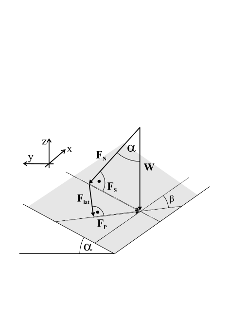
Figure 3: This figure illustrates vector decomposition in a more general case. The skier’s trajectory describes an angle $\beta$ with the horizontal and is explicitly indicated in the figure by the straight line parallel to $\bm{F}_{\rm P}$. The force $\bm{F}_{\rm S}$, which is acting inside the slope plane, is decomposed into a lateral force $\bm{F}_{\rm{lat}}$ and a force $\bm{F}_{\rm P}$ which is parallel to the skier’s trajectory and leads to an acceleration. Of course, the force $\bm{F}_{\rm N}$ is perpendicular to the slope.

For a skier’s trajectory directly in the fall line, we have $\beta=90^{o}$, $\bm{F}_{\rm{lat}}=0$ and $\bm{F}_{\rm S}=\bm{F}_{\rm P}$, resulting in maximum acceleration along the fall line. Let $\hat{\mathbf{f}}$ be a unit vector tangent to the skier’s trajectory, i.e.  $\hat{\mathbf{f}}\,||\,\bm{F}_{\rm P}$, and $\|\hat{\mathbf{f}}\|=1$. The direction of $\bm{F}_{\rm P}$ is displayed in figure 3. An analytic expression for $\hat{\mathbf{f}}$ can easily be obtained by starting from a unit vector $\hat{\bm{x}}$ as implied by the conventions used in figure 3. We first rotate $\hat{\bm{x}}$ about the $z$-axis by an angle $-\beta$, and obtain a vector $\hat{\mathbf{i}}$. A further rotation about the $x$-axis by an angle $+\alpha$ leads to the vector $\hat{\mathbf{f}}$.

Of course, a rotation of $\hat{\bm{x}}$ by $-\beta$ leads to $\hat{\mathbf{i}}=(\cos\beta,-\sin\beta,0)$. The rotation of $\hat{\mathbf{i}}$ about the $x$-axis by an angle $\alpha$, which “rotates $\hat{\mathbf{i}}$ into the ski slope”, is expressed as a rotation matrix,

$$R=\left(\begin{array}[]{ccc}1&0&0\\ 0&\cos\alpha&-\sin\alpha\\ 0&\sin\alpha&\sin\alpha\end{array}\right)\quad\Rightarrow\quad\hat{\mathbf{f}}=R\cdot\hat{\mathbf{i}}=\left(\begin{array}[]{c}\cos\beta\\ -\cos\alpha\sin\beta\\ -\sin\alpha\sin\beta\end{array}\right).$$ (11)

Then, by projection,

$$\bm{F}_{\rm P}=(\hat{\mathbf{f}}\cdot\bm{F}_{\rm S})\,\hat{\mathbf{f}}=-m\,g\,\left(\begin{array}[]{c}-\sin\alpha\,\sin\beta\,\cos\beta\\ \sin\alpha\,\cos\alpha\,\sin^{2}\beta\\ \sin^{2}\alpha\,\sin^{2}\beta\end{array}\right)\,,$$ (12)

and the modulus of the vector $\bm{F}_{\rm P}$ is

$$\|\bm{F}_{\rm P}\|=\|\bm{F}_{\rm S}\|\,|\sin\beta|\,=\,m\,g\,\sin\alpha\,|\sin\beta|\,.$$ (13)

The force $\bm{F}_{\rm{lat}}$ perpendicular to the track direction is then easily calculated with the help of equation (10),

$$\bm{F}_{\rm{lat}}=\bm{F}_{\rm S}-\bm{F}_{\rm P}=-m\,g\,\left(\begin{array}[]{c}\sin\alpha\,\sin\beta\,\cos\beta\\ \sin\alpha\,\cos\alpha\,\cos^{2}\beta\\ \sin^{2}\alpha\,\cos^{2}\beta\end{array}\right),\\$$ (14)

resulting in

$$\|\bm{F}_{\rm{lat}}\|=\|\bm{F}_{\rm S}\|\,|\cos\beta|=m\,g\,\sin\alpha\,|\cos\beta|\,.$$ (15)

This force has to be compensated by the snow, under the approximation of vanishing slippage.

2.4 Effective Weight

According to figure 3, the gravitational force may be decomposed as $\bm{W}=\bm{F}_{\rm N}+\bm{F}_{\rm{lat}}+\bm{F}_{\rm P}$. The force $\bm{F}_{\rm P}$ simply accelerates the skier. The force $\bm{F}_{\rm{load}}=\bm{F}_{\rm N}+\bm{F}_{\rm{lat}}$ therefore has to be compensated by the snow. Therefore, to avoid slippage, the skier should balance her/his weight in such a way that his/her center-of-mass is joined with the ski along a straight line parallel to the direction given by the effective weight vector $\bm{F}_{\rm{load}}$,

$$\bm{F}_{\rm{load}}=\bm{W}-\bm{F}_{\rm P}=\bm{F}_{\rm N}+\bm{F}_{\rm{lat}}\,.$$ (16)

We immediately obtain

$$\bm{F}_{\rm{load}}=m\,g\,\left(\begin{array}[]{c}-\sin\alpha\,\sin\beta\,\cos\beta\\ \sin\alpha\,\cos\alpha\,\sin^{2}\beta\\ \sin^{2}\alpha\sin^{2}\beta-1\end{array}\right)\,,\quad\|\bm{F}_{\rm{load}}\|=\sqrt{\bm{F}_{\rm N}^{2}+\bm{F}_{\rm{lat}}^{2}}=m\,g\,\sqrt{\sin^{2}\alpha\sin^{2}\beta+1}\,.$$ (17)

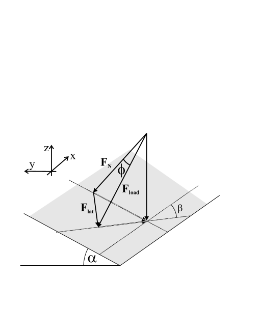
Figure 4: The skier’s trajectory is as indicated in figure 3. The effective weight of the skier is $\bm{F}_{\rm{load}}$. We remember that $\bm{F}_{\rm N}$ is perpendicular to the ski slope. In order to avoid slippage, the line joining the ski boots and the skier’s center-of-mass must be parallel to $\bm{F}_{\rm{load}}$. The tilt angle of the skier with the normal to the ski slope is equal to the angle of $\bm{F}_{\rm{load}}$ with $\bm{F}_{\rm N}$; this angle is denoted by the symbol $\phi$ in the text.

We call $\phi$ the angle of inclination or tilt angle. For obvious reasons, we assume this angle to be in the range $\phi\in[0^{o},90^{o}]$. The angle $\phi$ also enters in the inclination-dependent sidecut radius as given in equation (6). We now investigate the question how $\phi$ is related to $\alpha$ and $\beta$. To this end, we first calculate

$$\cos\phi=\frac{\bm{F}_{\rm{load}}\cdot\bm{F}_{\rm N}}{\|\bm{F}_{\rm{load}}\|\,\|\bm{F}_{\rm N}\|}=\frac{\cos\alpha}{\sqrt{\cos^{2}\alpha+\cos^{2}\beta\,\sin^{2}\alpha}}\,.$$ (18)

We now apply the identity $\tan[\cos^{-1}(x)]=\sqrt{1-x^{2}}/x$ to both sides of this equation. The left-hand side becomes just $\tan\phi$, and the right-hand side simplifies to $\tan\alpha\,|\cos\beta|$.

Alternatively, we observe that $\bm{F}_{\rm N}$, $\bm{F}_{\rm{lat}}$ and $\bm{F}_{\rm{load}}$ are vectors in one and the same plane. Because $\bm{F}_{\rm N}$ is perpendicular to the ski slope and $\bm{F}_{\rm{lat}}$ is a vector in the plane formed by the slope, both vectors are at right angles to each other (see figure 4). We immediately obtain

$$\tan\phi=\frac{\|\bm{F}_{\rm{lat}}\|}{\|\bm{F}_{\rm N}\|}=\frac{m\,g\,\sin\alpha\,|\cos\beta|}{m\,g\,\cos\alpha}=\tan\alpha\,|\cos\beta|\,.$$ (19)

2.5 Forces Acting in a Curve

In a turn (see figure 5), the centrifugal inertial force $\bm{F}_{\rm C}$,

$$\bm{F}_{\rm C}=\pm\,m\,\frac{v^{2}}{R}\,\frac{\bm{F}_{\rm{lat}}}{\|\bm{F}_{\rm{lat}}\|}\,,$$ (20)

has to be added to or subtracted from the lateral gravitational force $\bm{F}_{\rm{lat}}=\bm{F}_{S}-\bm{F}_{P}$ to obtain the total radial force, which we name $\bm{F}_{\rm{LAT}}$ in order to differentiate it from $\bm{F}_{\rm{lat}}$. In the second (“lower”) half of a left as well as in the second (“lower”) half of a right curve, the centrifugal force is parallel to the lateral force, and the positive sign prevails in equation (20). By contrast, in the upper half of either a curve, the centrifugal force is antiparallel to the lateral force, and the negative sign should be chosen. We have (see equations (8), (10) and 14))

$$\bm{F}_{\rm{LAT}}=\bm{F}_{\rm{lat}}+\bm{F}_{\rm C}\,.$$ (21)

The force $\bm{F}_{\rm{lat}}$ may be parallel or antiparallel to the centrifugal force, resulting in a different formula for $\bm{F}_{\rm{LAT}}$ in each case,

$$\|\bm{F}_{\rm{LAT}}\|=\left|m\frac{v^{2}}{R}\pm m\,g\sin\alpha\,|\cos\beta|\right|\,.$$ (22)

The new effective weight is

$$\bm{F}_{\rm{LOAD}}=\bm{F}_{\rm N}+\bm{F}_{\rm{LAT}}\,.$$ (23)

The tilt angle changes as we replace $\bm{F}_{\rm{load}}\to\bm{F}_{\rm{LOAD}}$. We denote the new tile angle by $\Phi$ as opposed to $\phi$ (see equation (19)). Using a relation analogous to (18),

$$\cos\Phi=\frac{\bm{F}_{\rm{LOAD}}\cdot\bm{F}_{\rm N}}{\|\bm{F}_{\rm{LOAD}}\|\,\|\bm{F}_{\rm N}\|}\,,$$ (24)

or by an elementary geometrical consideration (using the orthogonality of $\bm{F}_{\rm{LAT}}$ and $\bm{F}_{\rm N}$), we obtain

$$\tan\Phi=\left|\frac{v^{2}}{g\,R\,\cos\alpha}\,\pm\,\tan\alpha\,|\cos\beta|\right|\,.$$ (25)

Furthermore, we assume the skier’s velocity to be sufficiently large that the centrifugal force dominates the lateral force; in this case we have

$$m\,\frac{v^{2}}{R}>m\,g\sin\alpha\,|\cos\beta|\qquad\mbox{and}\qquad\frac{v^{2}}{g\,R\,\cos\alpha}>\tan\alpha\,|\cos\beta|$$ (26)

along the entire curve. In this case, for a right curve, with $\beta=0^{o}$ at the outset and $\beta=180^{o}$ at the end of the curve, and with $\cos\beta$ changing sign at $\beta=90^{o}$, the correct sign in equation (25) is

$$\tan\Phi=\frac{v^{2}}{g\,R\,\cos\alpha}-\tan\alpha\,\cos\beta\qquad\mbox{(fast skier, right curve)}\,.$$ (27)

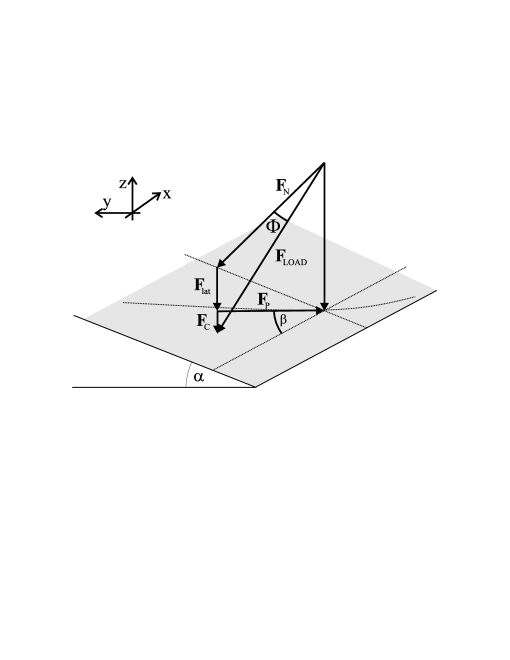
Figure 5: The total lateral force $\bm{F}_{\rm{LAT}}$ in a curve is the sum of $\bm{F}_{\rm{lat}}$ given in (14) and the centrifugal force $\bm{F}_{\rm C}$ defined in (20). This leads to a modified effective weight $\bm{F}_{\rm{LOAD}}$. For the centrifugal force to act as shown in the figure, the skier’s trajectory is required to describe a left-hand curve, as displayed.

3 The Ideal–Carving Equation

3.1 Derivation

Up to this point we have mainly followed the discussion outlined on pp. 76–104 and pp. 208–215 of [1]. Under the assumption of a perfect carved turn, the instantaneous curvature radius $R$, which is determined by the bent edges of the ski, depends on the sidecut radius $R_{\rm SC}$ and on the tilt angle $\Phi$ as follows (see equation (6)),

$$R(\Phi)=R_{\rm SC}\,\cos\Phi\,.$$ (28)

However, the assumption of a carved turn requires that the effective weight $\bm{F}_{\rm{LOAD}}$ be acting along the straight line joining the ski boots and the center-of-mass of the skier. This means that the angle $\Phi$ also has to fulfill the equation (25) which we specialize to the case (27) in the sequel,

$$\tan\Phi=\frac{v^{2}}{g\,R\,\cos\alpha}\,-\,\tan\alpha\,\cos\beta\,.$$ (29)

In view of (28), we have

$$\tan\Phi=\sqrt{\frac{R_{\rm SC}^{2}}{R^{2}}-1}\,.$$ (30)

Combining (29) and (30), we obtain the ideal-carving equation

$$\sqrt{\frac{R_{\rm SC}^{2}}{R^{2}}-1}=\frac{v^{2}}{g\,R\,\cos\alpha}-\tan\alpha\,\cos\beta\,.$$ (31)

The variables of the ideal-carving equation are the velocity $v$ of the skier, the angle $\beta$ of the trajectory of the skier with the horizontal, and the instantaneous curvature radius $R$ of the skier’s trajectory. The parameters of (31) are the inclination of the ski slope $\alpha$, the acceleration of gravity $g$, and the sidecut radius $R_{\rm SC}$ of the ski. Under appropriate substitutions, this equation is equivalent to equation (T5.3) on p. 209 of [1]. In contrast to [1], the tilt angle is eliminated from the equation in our formulation.

Alternatively speaking, the ideal-carving equation defines a function

$$f(v,R,\beta)=\frac{v^{2}}{g\,R\,\cos\alpha}-\tan\alpha\cos\beta-\sqrt{\frac{R_{\rm SC}^{2}}{R^{2}}-1}\,,$$ (32a)

so that the equation

$$f(v,R,\beta)=0$$ (32b)

defines the “ideal-carving surface” as a 2-dimensional imbedded in a three-dimensional space spanned by $v$, $R$, and $\beta$.

Likewise, we may consider the ideal-gas equation

$$p\,V\,=\,N\,k\,T$$ (33a)

where $$p V N k T$$ is the pressure, denotes the volume, the number of atoms, the Boltzmann constant, and the absolute temperature. The ideal-gas equation may trivially be rewritten as follows,

$$F(p,V,T)=\frac{pV}{NkT}\,-\,1\,=\,0\,.$$ (33b)

Of course, the equation $F(p,V,T)=0$ then defines a (two-dimensional) surface embedded in $\mathbbm{R}^{3}$. The ideal-gas equation entails the idealization of perfect thermodynamic equilibrium, yet in realistic processes a gas volume will not always be in such a state. Nevertheless, in order to avoid sub-optimal performance within a Carnot-like process (or by analogy: in order to avoid frictional losses when skiing), one may strive to keep the system as close to equilibrium as possible at all times.

3.2 Graphical Representation

The solutions of (32) define a (two-dimensional) surface embedded in $\mathbbm{R}\times\mathbbm{R}\times[0^{o},180^{o}]$. In figure 6, the surface defined by equation (32b) is represented for the parameter combination $R_{\rm SC}=16~{}{\rm m}$, $g=9.81~{}{\rm m}/{\rm s}^{2}$, and $\alpha=15^{o}$.

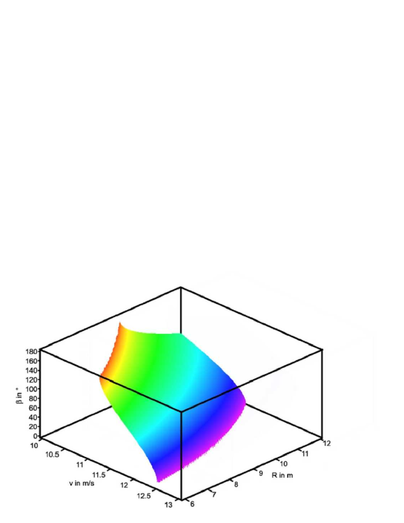
Figure 6: The ideal-carving manifold for the parameters $R_{\rm SC}=16~{}{\rm m}$, $g=9.81~{}{\rm m}/{\rm s}^{2}$, and $\alpha=15^{o}$. The variables are the skier’s velocity $v$, the instantaneous radius of curvature $R$, and the angle $\beta$ of the skier’s trajectory with the horizontal.

Figure 6 gives us rather important information. In particular, we see that maintaining the ideal-carving condition while going through a curve of constant radius of curvature, within the interval $\beta=0^{o}$ to $\beta=180^{o}$, implies a decrease in the skier’s speed. This is possible only if the frictional force, antiparallel to $\bm{F}_{\rm P}$, provides for sufficient deceleration. Of course, under ideal racing conditions the skier will accelerate rather than decelerate during her/his descent.

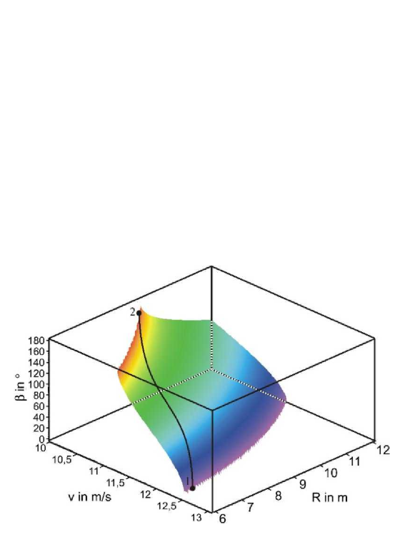
Figure 7: A hypothetical trajectory of a skier maintaining the ideal-carving condition (32) during a right turn. Parameters are the same as in figure 6. Note that the skier’s velocity decreases from $v\approx 12.5\,{\rm m}/{\rm s}$ to $v\approx 10.5\,{\rm m}/{\rm s}$ during the turn.

Acceleration during a turn is compatible with the ideal carving condition only if the instantaneous radius of curvature significantly decreases during the turn. This corresponds to a turn in which the skier starts off with a very wide turn, gradually making the turn more tight during his/her descent. The pattern generated is that of the letter “J”, and the corresponding curve is therefore commonly referred to as a “J-curve” [1]. The practical necessities of world-cup racing prevent such trajectories. Typical tilt angles are too high, and typical centrifugal forces too large to be sustainable in practice on the idealized trajectories. This is why we see snow spraying even in highly competitive world-cup slalom and giant slalom skiing.

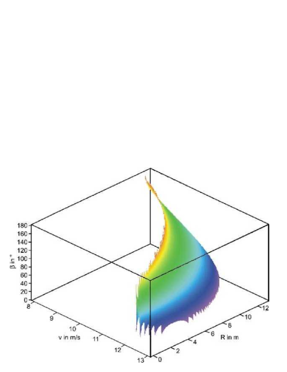
Figure 8: The ideal-carving manifold in the range of small $R$. Parameters are the same as figures 6 and 7.

However, there is yet another very important restriction to the possibility of maintaining ideal-carving conditions at all times: An inspection of figures 6 and 7 suggests that for an appreciable radius of curvature, the velocity $v$ decreases monotonically with the radius, $\beta$ being held constant. We now investigate the specific velocity compatible with ideal-carving conditions at very tight turns $R\to 0$. The tilt angle $\Phi$ tends to values close to $90^{o}$ in this case, because

$$\lim_{R\rightarrow 0}\tan\Phi=\lim_{R\rightarrow 0}\sqrt{\frac{R_{\rm SC}^{2}}{R^{2}}-1}\to\infty\qquad\mbox{as}\qquad R\to 0\,.$$ (34)

Solving equation (31) for $v$, we obtain

$$v(R,\beta)=\sqrt{g\,R\,\cos\alpha}\,\sqrt{\sqrt{\frac{R_{\rm SC}^{2}}{R^{2}}-1}+\tan\alpha\cos\beta}\to\sqrt{g\,R_{\rm SC}\,\cos\alpha}\qquad\mbox{as}\qquad R\to 0\,.$$ (35)

This latter relation holds independent of $\beta$, and this virtual independence of $\beta$ is represented graphically in figure 8 for small $R$. As suggested by figures 6 and 7, it is impossible to maintain ideal-carving conditions if the skier’s velocity considerably exceeds the limiting velocity

$$v_{\rm limit}=\sqrt{g\,R_{\rm SC}\,\cos\alpha}\,.$$ (36)

We investigate this question in more detail. For given $R$, the maximum $v$ is attained for $\beta=0$ because in this case, the centrifugal force is most effectively compensated by the lateral force $\bm{F}_{\rm{lat}}$. In this case,

$$v(R,0) = \sqrt{g\,R\,\cos\alpha}\,\sqrt{\sqrt{\frac{R_{\rm SC}^{2}}{R^{2}}-1}+\tan\alpha}$$ (37)

$$= v_{\rm limit}\,\left(1+\tan(\alpha)\,\left(\frac{R}{R_{\rm SC}}\right)-\frac{2+\tan^{2}(\alpha)}{8}\,\left(\frac{R}{R_{\rm SC}}\right)^{2}+{\cal O}(R^{2})\right)\,.$$

The maximum $v$ for which the ideal-carving condition can possibly be fulfilled is then determined by the condition

$$\left.\frac{\partial v}{\partial R}\right|_{\beta=0}=0\,,$$ (38)

which, upon considering the first two nonvanishing terms in the Taylor expansion (37) for small $R/R_{\rm SC}$, leads to

$$R_{\rm max}\approx\frac{2\,\tan\alpha}{2+\tan^{2}\alpha}\,R_{\rm SC}=R_{\rm SC}\,\left(\alpha-\frac{\alpha^{3}}{6}+{\cal O}(\alpha^{5})\right)\,,$$ (39a)

a result which happens to be exact up to the order of $$\alpha^{5}$$. The exact solution is surprisingly simple,

$$R_{\rm max}=R_{\rm SC}\,\sin\alpha\,.$$ (39b)

The maximum velocity compatible with ideal-carving conditions is independent of $\alpha$,

$$v_{\rm max}=v(R_{\rm max},0)=\sqrt{g\,R_{\rm SC}}\,.$$ (40)

It implies a tilt angle $\Phi=90^{o}-\alpha$ at $\beta=0$. The velocity $v_{\rm max}$, of course, equals the velocity of a body on a circular trajectory of radius $R_{\rm SC}$ with the centrifugal force being compensated by an acceleration of magnitude $g$ toward the center. Observe, however, that in the current case the instantaneous radius of curvature is $R_{\rm SC}\,\sin\alpha$.

A numerical example: For $R_{\rm SC}=14\,{\rm m}$, and $\alpha=30^{o}$, we have $R_{\rm max}=7\,{\rm m}$ and $v_{\rm max}=11.72\,{\rm m}/{\rm s}$. The limiting velocity deviates by about $10\,\%$ and is given by $v_{\rm limit}=10.91\,{\rm m}/{\rm s}$.

Both the limiting velocity $v_{\rm limit}$ as well as the maximum velocity $v_{\rm max}$ are given purely as a function of the parameters of the ideal-carving equation (31): these are the acceleration of gravity $g$, the sidecut radius $R_{\rm SC}$, and the inclination of the ski slope $\alpha$. Furthermore, we observe that for typical parameters as given in figure 8, the ideal velocity of the skier varies only within about $30\,\%$ for all radii of curvature in the interval $[0\,{\rm m},12\,{\rm m}]$, and all possible $\beta$. That is to say, the limiting $v_{\rm limit}$ also gives a good indication of the velocity range under which a carving ski, or a snowboard, can operate under nearly ideal-carving conditions (see also figure 9).

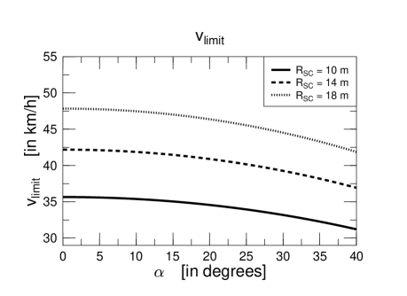
Figure 9: The limiting velocity $v_{\rm limit}$ [Eq. (36)] is displayed for typical inclinations of the ski slope $\alpha$. For velocities appreciably beyond $v_{\rm limit}\approx v_{\rm max}$ [see Eqs. (36) and (40)], it is impossible to maintain ideal-carving conditions.

4 Implications and Conclusions

In section 2, we have discussed in detail the forces acting on a skier during a carved turn, as well as basic geometric properties of carving skis and snowboards. In section 3, We have discussed in detail the derivation of the ideal-carving equation (31) which establishes a relation between the skier’s velocity, the radius of curvature of the skier’s trajectory and the angle of the skier’s course with the horizontal. This equation determines an ideal-carving manifold whose properties have been discussed in section 3.2, with graphical representations for typical parameters to be found in figures 6—9. In particular, the limiting velocity $v_{\rm limit}$ as given in equation (36) indicates an ideal operational velocity of a carving ski as a function of the angle of inclination of the ski slope and of the sidecut radius.

The range of the limiting velocities indicated in figure 9 are well below those attained in world-cup downhill skiing. In downhill skiing, the usage of skis with an appreciable sidecut is therefore not indicated. However, the velocity range of figure 9 is well within the typical values attained in slalom races. It is therefore evident that carving skis are well suited for such races, in theory as well as in practice. A slalom with tight turns, which implies a rather slow operational velocity due to the necessity of changing the trajectory within the reaction time of a human being, demands slalom skis with a smaller sidecut radius than those suited for a rather flat slope and wide turns. Note that a smaller sidecut radius implies a larger actual sidecut $d$ according to equation (3). It may well be beneficial for a slalom skier to have a look at the actual course, and to measure the average steepness of the slope, and to choose an appropriate ski from a given selection, before starting her/his race.

We will now discuss possible further improvements in the design of carving skis. To this end we draw an analogy to the steering of a bicycle traveling on an inclined surface. The driver is supposed not to exert any force via the action of the pedals of the bicycle. Indeed, during the ride on a bicycle, the driver can maintain ideal-“carving” conditions under rather general circumstances, avoiding slippage. One might ask why a bicycle driver can accomplish this while a carving skier or snowboarder cannot. The reason is the following: Equation (28) defines a relation between the tilt angle $\Phi$ and the instantaneous radius of curvature $R$. When riding a bicycle, one may freely adjust the relation between $\Phi$ and $R$ via the steering. On carving skis, the position of the “steering” is always uniquely related to the tilt angle $\Phi$ by equation (28). On a bicycle, it is possible to use a small steering angle even if one leans substantially toward the center of the curve. On a carving ski, the “steering angle” automatically becomes large when the tilt angle is large, resulting in a small radius of curvature (again under the assumption of “ideal-carving” conditions). This circumstance eventually leads to the limiting velocity $v_{\rm limit}$ beyond which it is impossible to operate a carving ski under ideal-carving conditions, as represented by equation (40). Beyond the limiting velocity, the non-fulfillment of the ideal-carving equation is visible by spraying snow. By contrast, on a bicycle, it is possible to adjust the steering of the front wheel so that the radius of curvature as defined by the relative inclination of the front and rear wheels, and the inclination $\Phi$ of the bicycle itself, fulfill the ideal-carving equation (31).

A carving ski that offers the possibility of steering could be constructed with the help of an inertial measurement device (see e.g. [2]). This device is supposed to continuously read the tilt angle $\Phi$, the velocity of the skier $v$ and the instantaneous radius of curvature $R$, as well as the angle $\beta$ and the inclination of the ski slope $\alpha$. According to equation (31), these variables determine an ideal sidecut radius $R_{\rm SC}$ which could be adjusted dynamically by a servo motor. In this case, it would be possible to fulfill near-ideal-carving conditions along the entire trajectory. A first step in this direction would be simpler device that measures only the inclination of the ski slope $\alpha$ and determines a near-ideal sidecut radius according to equation (36).

References

- [1] D. Lind and S. P. Sanders, The Physics of Skiing (Springer, New York, 1996).
- [2] For a brief overview see e.g. U. Kilian, Physics Journal (“Physik Journal” of the German Physical Society) 2 (October issue), 56 (2003). Simplified inertial measurement system are currently used in devices as small as computer mice. They are usually called “gyroscopes” in the literature although the technical realization is sometimes based on different principles (for example, optical gyroscopes or micromechanical devices).