Abstract

Influence of the plate surfaces roughness in precise ellipsometry experiments is studied. The realistic case of a Gaussian laser beam crossing a uniaxial platelet is considered. Expression for the transmittance is determined using the first order perturbation theory. In this frame, it is shown that interference takes place between the specular transmitted beam and the scattered field. This effect is due to the angular distribution of the Gaussian beam and is of first order in the roughness over wavelength ratio. As an application, a numerical simulation of the effects of quartz roughness surfaces at normal incidence is provided. The interference term is found to be strongly connected to the random nature of the surface roughness.

1 Introduction

The high-accuracy universal polarimeter (HAUP) [1] has proved to be a very useful instrument to measure the crystal optical properties (see for instance [2, 3, 4] and references therein). The principle is simple and was introduced a long time ago (see [5] for an historical introduction): the light intensity measured after a rotating high quality polariser, a crystal plate (the sample) and a high quality rotating analyser, is fitted to a theoretical formula with several coefficients as free parameters where the delay due to birefringence and optical activity can be determined.

The accuracy of this instrument has now reached the few $10^{-5}$ level and systematic errors contributing at this order of magnitude have been investigated [6, 7, 8]. The conclusion is that roughness is most likely one of the main source of systematic uncertainties.

However, despite an extensive literature on surface roughness [9, 10], no theoretical expression for the transmission of a Gaussian beam by an anisotropic rough platelet is available. It is the purpose of this article to provide this expression. We consistently take into account the Gaussian nature of the laser beam, the multiple reflection inside the plate and the roughness of both faces of the plate. To simplify the calculations we further restrict ourselves to uniaxial homogeneous crystals. As a result, we find that unlike plane waves, specular Gaussian beams are affected by the surfaces roughness, even in the first order perturbation theory.

The physical origin of this phenomenon is the angular distribution, or plane wave expansion, of Gaussian beams [11]. Plane waves constituting a Gaussian beam having different wave vectors, a given plane wave can then be scattered in the specular direction of the other ones. The resulting interference pattern leads to an a priori non vanishing contribution of the scattered field in the specular region. To some extent, this phenomenon is thus related to the near-specular scattering by rough surfaces introduced in [12].

Another aspect of realistic platelet surfaces is the interface parallelism default. Depending on the wedge angle, this default can compete with roughness in the modifications of the transmitted beam polarisation. The nature of these effects is however different. Given the relative orientation of the two plate interfaces, the wedge effect is univocal whereas roughness, as it will be shown in this paper, is of random nature. It is then most likely that these two effects cannot compensate each other. In principle, the perturbative calculations reported in the present article holds for both effects. Nevertheless, the boundary matching method, applied a long time ago to isotropic wedges [13], can be used to describe the wedge effect. We shall report this calulation in a future publication and restrict ourselves here on platelet roughness.

This article is organised as follows. In section 2 we derive the theoretical expressions and numerical simulations of quartz plates are presented in section 3.

2 Formalism

The choice of the theoretical formalism is driven by the properties of the crystal plate surfaces under study. Fortunately, an exhaustive experimental study on crystal surfaces has recently been published [14]. Most of the high quality polished crystal surfaces used in optics have a profile surface correlation length of the order of the optical wavelength and a root mean square roughness of the order of a few angstrœm. It means that one can safely use a first order perturbation theory [15] neglecting the local field effects[16]. The more suitable formalism for our problem is the one introduced in [17] and generalised to anisotropic overlayers in [18]. However, in the latter reference, the anisotropy is treated perturbatively and only the reflection of plane waves is considered. We shall then extend this formalism to platelet’s transmission taking fully into account the plate anisotropy and treating perturbatively the plate roughness.

In the following we tried to be concise, referring to [17, 18] for further details. The wave equation corresponding to the system represented in figure 1 is:

$$\bf{\nabla}\times\bf{\nabla}\times\bf{E}(\bf{r})=\omega^{2}\mu_{0}\bf{D}(\bf{r})$$ (1)

with $\bf{D}(\bf{r})={\cal E}(z)\bf{E}(\bf{r})$ and

$${\cal E}(z)=\Theta\biggl{(}-z+h_{0}(x,y)\biggr{)}\epsilon_{0}{\underline{1}}+\biggl{[}\Theta\biggl{(}z-h_{0}(x,y)\biggr{)}-\Theta\biggl{(}z-a-h_{a}(x,y)\biggr{)}\biggr{]}{\underline{\epsilon}}$$

$$+\Theta\biggl{(}z-a-h_{a}(x,y)\biggr{)}\epsilon_{0}{\underline{1}}$$ (2)

where ${\underline{1}}$ is the $3\times 3$ identity matrix and $\Theta$ is the Heaviside function. For uniaxial media, it is useful to write [19]

$${\underline{\epsilon}}=\epsilon_{\perp}{\underline{1}}+(\epsilon_{\parallel}-\epsilon_{\perp})\mbox{${\rm\bf\hat{c}}$}\mbox{${\rm\bf\hat{c}}$}$$

with $\mbox{${\rm\bf\hat{c}}$}^{T}=\{c_{x},c_{y},c_{z}\}$ the unit vector along the optical axis, ${\rm\bf\hat{c}}$${\rm\bf\hat{c}}$ a Dyad and $\epsilon_{\perp}=n_{o}^{2}\epsilon_{0}$, $\epsilon_{\parallel}=n_{e}^{2}\epsilon_{0}$ the ordinary and extraordinary components of the dielectric tensor. In equation (2), the two functions $h_{0}(x,y)$ and $h_{a}(x,y)$ are the profiles of the two surfaces located at $z=0$ and $z=a$ respectively. As usual [20], we assume that the two planes $z=0$ and $z=a$ are defined such that the mean profiles vanish, i.e. $<h_{0}>=<h_{a}>=0$.

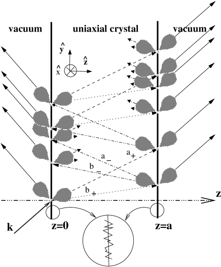
Figure 1: Schematic view of the plane wave propagation in the anisotropic slab. For the sake of clarity, some of the inner reflected rays are represented by small arrows. The plane of incidence coincides with the plane $yz$. Symbols $a_{\pm}$ and $b_{\pm}$ correspond to the four possible propagation directions inside the medium. The vector basis $\{\mbox{${\rm\bf\hat{x}}$},\mbox{${\rm\bf\hat{y}}$},\mbox{${\rm\bf\hat{z}}$}\}$ used throughout this article is also shown. The grey areas symbolise the scattered light due to surfaces roughness.

The solution of equation (1) can be written $\bf{E}(\bf{r})=\bf{E}_{0}(\bf{r})+\bf{E^{\prime}}(\bf{r})$ with $\bf{E}_{0}(\bf{r})$ given by the zero order wave equation

$$\bf{\nabla}\times\bf{\nabla}\times\bf{E}_{0}(\bf{r})=\omega^{2}\mu_{0}\bf{D}_{0}(\bf{r})$$ (3)

where ${\bf D_{0}}({\bf r})={\cal E}_{0}(z){\bf E_{0}}({\bf r})$ and

$${\cal E}_{0}(z)=\Theta(-z)\epsilon_{0}{\underline{1}}+\biggl{(}\Theta(z)-\Theta(z-a)\biggr{)}{\underline{\epsilon}}+\Theta(z-a)\epsilon_{0}{\underline{1}}.$$ (4)

To first order in $\omega h/c$ [18], one has ${\cal E}(z)={\cal E}_{0}(z)+\delta{\cal E}(z)$ with

$$\delta{\cal E}(z)\approx\biggl{(}h_{a}(x,y)\delta(z-a)-h_{o}(x,y)\delta(z)\biggr{)}\biggl{[}(\epsilon_{\perp}-\epsilon_{0}){\underline{1}}+(\epsilon_{\parallel}-\epsilon_{\perp})\mbox{${\rm\bf\hat{c}}$}\mbox{${\rm\bf\hat{c}}$}\biggr{]}$$ (5)

with $\delta(z)$ the Dirac distribution.

To derive the differential equation for the first order scattered field $\bf{E^{\prime}}(\bf{r})$, we introduce the Fourier transform

$${\bf E}({\bf K};z)={\cal F}[{\bf E}({\bf r})]=\frac{1}{2\pi}\int{\bf E}({\bf r})\exp(i{\bf K}\cdot{\bf R}){\rm d}^{2}{\bf R}$$

where ${\bf R}=({\bf r}\cdot\mbox{${\rm\bf\hat{x}}$})\mbox{${\rm\bf\hat{x}}$}+({\bf r}\cdot\mbox{${\rm\bf\hat{y}}$})\mbox{${\rm\bf\hat{y}}$}$ and ${\bf K}=({\bf k}\cdot\mbox{${\rm\bf\hat{x}}$})\mbox{${\rm\bf\hat{x}}$}+({\bf k}\cdot\mbox{${\rm\bf\hat{y}}$})\mbox{${\rm\bf\hat{y}}$}$ with ${\bf k}$ the wave vector. Here, since we are considering Gaussian beams, no spatial length is introduced in the Fourier transformation.

Taking the Fourier transform of equations (1) and (3) and then subtracting them, one obtains[18]

$$\biggl{(}-i{\bf K}+\mbox{${\rm\bf\hat{z}}$}\frac{\partial}{\partial z}\biggr{)}\biggl{(}-i{\bf K}\cdot{\bf E^{\prime}}({\bf K};z)+\frac{\partial E^{\prime}_{z}({\bf K};z)}{\partial z}\biggr{)}-\biggl{(}-K^{2}+\frac{\partial^{2}}{\partial z^{2}}\biggr{)}{\bf E^{\prime}}({\bf K};z)=\omega^{2}\mu_{0}{\bf D^{\prime}}({\bf K};z),$$ (6)

with ${\bf D^{\prime}}({\bf K};z)={\bf D}({\bf K};z)-{\bf D}_{0}({\bf K};z)$. For perturbative stability, the wave equation must be written as a function of the continuous electric field components [17], that is $E^{\prime}_{x}$, $E^{\prime}_{y}$ and $D^{\prime}_{z}$. We shall do it separately for the $s$ and $p$ scattered waves as in [17]. However, before providing the solutions we introduce[18] the following useful vector function:

$${\bf F}({\bf r})={\bf D}({\bf r})-{\cal E}_{0}(z){\bf E}({\bf r})=\delta{\cal E}(z){\bf E}({\bf r})\Leftrightarrow{\bf F}({\bf r})={\bf D^{\prime}}({\bf r})-{\cal E}_{0}(z){\bf E^{\prime}}({\bf r}),$$ (7)

which gathers the infinitesimal contributions to the perturbated wave equation. To first order, one gets:

$$F_{x}({\bf r})\approx\frac{1}{{\cal E}_{zz}(z)}\biggl{(} \delta{\cal E}_{xz}(z)D_{z}(\mbox{ ${\rm\bf r}$})+\biggl{[}{\cal E}_{zz}(z)\delta{\cal E}_{xx}(z)-{\cal E}_{xz}(z)\delta{\cal E}_{xz}(z)\biggr{]}E_{x}(\mbox{ ${\rm\bf r}$})+$$ (8)

$$\biggl{[}{\cal E}_{zz}(z)\delta{\cal E}_{xy}(z)-{\cal E}_{yz}(z)\delta{\cal E}_{xz}(z)\biggr{]}E_{y}(\mbox{ ${\rm\bf r}$})\biggr{)}\,,$$

$$F_{y}({\bf r})\approx\frac{1}{{\cal E}_{zz}(z)}\biggl{(} \delta{\cal E}_{yz}(z)D_{z}(\mbox{ ${\rm\bf r}$})+\biggl{[}{\cal E}_{zz}(z)\delta{\cal E}_{xy}(z)-{\cal E}_{xz}(z)\delta{\cal E}_{yz}(z)\biggr{]}E_{x}(\mbox{ ${\rm\bf r}$})+$$ (9)

$$\biggl{[}{\cal E}_{zz}(z)\delta{\cal E}_{yy}(z)-{\cal E}_{yz}(z)\delta{\cal E}_{yz}(z)\biggr{]}E_{y}(\mbox{ ${\rm\bf r}$})\biggr{)}\,,$$

$$F_{z}({\bf r})\approx\frac{1}{{\cal E}_{zz}(z)}\biggl{(} \delta{\cal E}_{zz}(z)D_{z}(\mbox{ ${\rm\bf r}$})+\biggl{[}{\cal E}_{zz}(z)\delta{\cal E}_{xz}(z)-{\cal E}_{xz}(z)\delta{\cal E}_{zz}(z)\biggr{]}E_{x}(\mbox{ ${\rm\bf r}$})+$$ (10)

$$\biggl{[}{\cal E}_{zz}(z)\delta{\cal E}_{yz}(z)-{\cal E}_{yz}(z)\delta{\cal E}_{zz}(z)\biggr{]}E_{y}(\mbox{ ${\rm\bf r}$})\biggr{)}\,.$$

where ${\cal E}_{ij}(z)$ and and $\delta{\cal E}_{ij}(z)$ are the components of the symmetric dielectric tensors of equations (2) and (5). In the leading order perturbation theory, one further set[17] $E_{x}(\mbox{ ${\rm\bf r}$})\approx E_{0x}(\mbox{ ${\rm\bf r}$})$, $E_{y}(\mbox{ ${\rm\bf r}$})\approx E_{0y}(\mbox{ ${\rm\bf r}$})$ and $D_{z}(\mbox{ ${\rm\bf r}$})\approx D_{0z}(\mbox{ ${\rm\bf r}$})$ in equations (8-10).

2.1 $p$ scattered wave

Projecting equation (6) onto ${\rm\bf\hat{z}}$ and utilising ${\bf\nabla}\cdot{\bf D}=0$ and equation (7), we obtain the $p$ wave equation:

$$-\frac{\partial}{\partial z}\frac{1}{\epsilon_{0}(z)}\frac{\partial D^{\prime}_{z}({\bf K};z)}{\partial z}-\omega^{2}\mu_{0}D^{\prime}_{z}({\bf K};z)+$$

$$i({\bf K}\cdot\mbox{${\rm\bf\hat{c}}$})\frac{\partial}{\partial z}\biggl{[}\frac{\Delta(z)}{\epsilon_{0}(z){\cal E}_{zz}(z)}\biggl{(}c_{z}D^{\prime}_{z}({\bf K};z)+\epsilon_{0}(z)\biggl{[}c_{x}E^{\prime}_{x}({\bf K};z)+c_{y}E^{\prime}_{y}({\bf K};z)\biggr{]}\biggr{)}\biggr{]}+$$

$$\frac{K^{2}}{{\cal E}_{zz}(z)}\biggr{(}D^{\prime}_{z}({\bf K};z)-{\cal E}_{xz}(z)E^{\prime}_{x}({\bf K};z)-{\cal E}_{yz}(z)E^{\prime}_{y}({\bf K};z)\biggr{)}$$

$$=\frac{\partial}{\partial z}\frac{1}{\epsilon_{0}(z)}\biggl{(}-i{\bf K}\cdot{\bf F}({\bf K};z)+i\frac{\Delta(z)}{{\cal E}_{zz}(z)}({\bf K}\cdot\mbox{${\rm\bf\hat{c}}$})c_{z}F_{z}({\bf K};z)\biggr{)}$$

$$+\frac{K^{2}}{{\cal E}_{zz}(z)}F_{z}({\bf K};z)$$ (11)

where we introduced $\epsilon_{0}(z)=\biggl{[}\Theta(-z)+\Theta(z-a)\biggr{]}\epsilon_{0}+\biggl{[}\Theta(z)-\Theta(z-a)\biggr{]}\epsilon_{\perp}$ and $\Delta(z)=\biggl{[}\Theta(z)-\Theta(z-a)\biggr{]}(\epsilon_{\parallel}-\epsilon_{\perp})$ such that equation (4) reads ${\cal E}_{0}(z)=\epsilon_{0}(z){\underline{1}}+\Delta(z)\mbox{${\rm\bf\hat{c}}$}\mbox{${\rm\bf\hat{c}}$}$.

Solutions of equation (11) are obtained using the Green’s functions[17, 18]. There exist, a priori, nine Green’s functions and thanks to the Dirac distributions appearing in equation (5), they must only be determined for $z^{\prime}=0$ and for $z^{\prime}\geq a$ (we remind that we are interested by the solution in the region $z\gg a$). Furthermore, for $z\gg a$ and $z<0$, all terms of equation (11) is front of the field components $E^{\prime}_{x}({\bf K};z)$ and $E^{\prime}_{y}({\bf K};z)$ vanish. Hence, the wave equation being expressed as function of the continuous field components, only one non zero Green’s function $G_{p}({\bf K};z,z^{\prime})$ exists[17, 18] in the two relevant regions $z>a^{\prime}$, $z^{\prime}\leq 0$ and $z>z^{\prime}$, $z^{\prime}\geq a$. The solution of equation (11) therefore reads:

$$D^{\prime}_{z}({\bf K};z)=\int_{-\infty}^{\infty}G_{p}({\bf K};z,z^{\prime})\biggl{(}\frac{\partial}{\partial z^{\prime}}\frac{1}{\epsilon_{0}(z^{\prime})}\biggl{[}-i{\bf K}\cdot{\bf F}({\bf K};z^{\prime})+i\frac{\Delta(z^{\prime})}{{\cal E}_{zz}(z^{\prime})}({\bf K}\cdot\mbox{${\rm\bf\hat{c}}$})c_{z}F_{z}({\bf K};z^{\prime})\biggr{]}$$

$$+\frac{K^{2}}{{\cal E}_{zz}(z^{\prime})}F_{z}({\bf K};z^{\prime})\biggr{)}{\rm d}z^{\prime}\,,$$ (12)

for $z>a$, where the Green’s function is given by [21]

$$G_{p}({\bf K};z,z^{\prime})=\frac{1}{W}\biggl{(}E_{p}^{<}({\bf K};z)E_{p}^{>}({\bf K};z^{\prime})\Theta(z^{\prime}-z)+E_{p}^{>}({\bf K};z)E_{p}^{<}({\bf K};z^{\prime})\Theta(z-z^{\prime})\biggr{)}$$ (13)

with

$$W=E_{p}^{<}({\bf K};z)\frac{\partial E_{p}^{>}({\bf K};z)}{\partial z}-E_{p}^{>}({\bf K};z)\frac{\partial E_{p}^{<}({\bf K};z)}{\partial z}$$

according to a theorem that can be found in [22]. Here $E_{p}^{<}({\bf K};z)$ and $E_{p}^{>}({\bf K};z)$ are the two independent plane-wave solutions of the unperturbated equation (3): $E_{p}^{>}({\bf K};z)$ corresponds to a wave coming from $z\rightarrow-\infty$ and $E_{p}^{<}({\bf K};z)$ to a wave coming from $z\rightarrow+\infty$. They are thus defined by the following boundary conditions:

$$\lim_{z\rightarrow+\infty}E_{p}^{>}({\bf K};z)\propto\exp(-ik_{z}z)$$

$$\lim_{z\rightarrow-\infty}E_{p}^{<}({\bf K};z)\propto\exp(ik_{z}z)\,.$$

with $k_{z}=+(k^{2}-K^{2})^{1/2}$.

Integrating by part the first term in the integral of equation (2.1) and using equations (8-10), one gets

$$E^{\prime}_{p}({\bf K};z)= \pi\biggl{\{}-i{\bf\hat{K}}\cdot\mbox{${\rm\bf\hat{c}}$}\Delta_{n}\biggl{(}1+\frac{1}{n_{o}^{2}(n_{o}^{2}+\Delta_{n}c_{z}^{2})^{2}}\biggr{)}c_{z}\widetilde{D^{p}_{z}}^{\prime}({\bf K})$$

$$-i\frac{n_{o}^{4}-1}{n_{o}^{2}}\biggl{(}{\bf\hat{K}}\cdot\mbox{${\rm\bf\hat{x}}$}\widetilde{E^{p}_{x}}^{\prime}({\bf K};z)+{\bf\hat{K}}\cdot\mbox{${\rm\bf\hat{y}}$}\widetilde{E^{p}_{y}}^{\prime}({\bf K};z)\biggr{)}$$

$$-i\frac{\Delta_{n}{\bf\hat{K}}\cdot\mbox{${\rm\bf\hat{c}}$}}{n_{o}^{2}+\Delta_{n}c_{z}^{2}}\biggl{[}1+n_{o}^{2}+\Delta_{n}c_{z}^{2}\biggl{(}1-\frac{1}{n_{o}^{2}(n_{o}^{2}+\Delta_{n}c_{z}^{2})}\biggr{)}\biggr{]}$$

$$\times\biggr{(}\widetilde{E^{p}_{x}}^{\prime}({\bf K})c_{x}+\widetilde{E^{p}_{y}}^{\prime}({\bf K})c_{y}\biggr{)}$$

$$+K\biggl{[}1+\frac{1}{(n_{o}^{2}+\Delta_{n}c_{z}^{2})^{2}}\biggr{]}\biggl{(}\biggl{[}n_{o}^{2}-1+\Delta_{n}c_{z}^{2}\biggr{]}\widetilde{D_{z}}({\bf K};z)$$

$$+c_{z}\Delta_{n}\biggl{[}c_{x}\widetilde{E^{p}_{x}}({\bf K};z)+c_{y}\widetilde{E^{p}_{y}}({\bf K};z)\biggr{]}\biggr{)}\biggr{\}}$$ (14)

for $z>a$ and with $\Delta_{n}=n_{e}^{2}-n_{o}^{2}$ and ${\bf\hat{K}}=(K_{x}\mbox{${\rm\bf\hat{x}}$}+K_{y}\mbox{${\rm\bf\hat{y}}$})/K$. To obtain this expression, we used the definition ${\bf E}^{\prime}_{p}({\bf K};z)=k/K{\bf E}^{\prime}_{z}({\bf K};z)$ with ${\bf\hat{K}}=\mbox{${\rm\bf\hat{y}}$}$ when $K=0$ [18] (see figure 1 for the definition of the reference axes). To shorten equation (14) we also introduced

$$\widetilde{D^{p}_{z}}({\bf K};z)= G_{p}({\bf K};z,a){\cal F}\biggl{[}D_{0z}({\bf R};a)\frac{h_{a}({\bf R})}{\lambda}\biggr{]}-$$

$$G_{p}({\bf K};z,0){\cal F}\biggl{[}D_{0z}({\bf R};0)\frac{h_{0}({\bf R})}{\lambda}\biggr{]}$$ (15)

$$\widetilde{D^{p}_{z}}^{\prime}({\bf K};z)= \frac{{\rm d}G_{p}({\bf K};z,z^{\prime})}{{\rm d}z^{\prime}}\biggr{|}_{z^{\prime}=a}{\cal F}\biggl{[}D_{0z}({\bf R};a)\frac{h_{a}({\bf R})}{\lambda}\biggr{]}-$$

$$\frac{{\rm d}G_{p}({\bf K};z,z^{\prime})}{{\rm d}z^{\prime}}\biggr{|}_{z^{\prime}=0}{\cal F}\biggl{[}D_{0z}({\bf R};0)\frac{h_{0}({\bf R})}{\lambda}\biggr{]}$$ (16)

where $\lambda$ is the laser wavelength. Identical expressions hold for $\widetilde{E^{p}_{x}}({\bf K})$, $\widetilde{E^{p}_{y}}({\bf K})$, $\widetilde{E^{p}_{x}}^{\prime}({\bf K})$ and $\widetilde{E^{p}_{y}}^{\prime}({\bf K})$ .

To derive equation (14) we assumed that [23]

$$\int_{-\infty}^{\infty}f(z)\delta(z){\rm d}z=\frac{1}{2}\biggl{[}\lim_{z\rightarrow 0^{+}}f(z)+\lim_{z\rightarrow 0^{-}}f(z)\biggr{]}$$ (17)

where $f(z)$ is a discontinuous function, but with a finite jump. Although this expression is not mathematically justified as stated in [23], it can however be used by considering that the Heaviside functions of equations (2,4) are given by the limit

$$\Theta(z)=\lim_{\zeta\rightarrow 0}[1+{\rm tanh}(z/\zeta)]/2\,.$$

This choice is justified by the freedom existing in the determination of the dielectric tensor at $z=0$ [24]. It is to mention that equation (17) leads to a disagreement with the boundary matching method for isotropic-isotropic interfaces in the case of oblique incidence. Another prescription was proposed in [25] to avoid this discrepancy. But, as mentioned in [26], no general proof was provided in [25]. There is then no reason for this particular prescription to work also for isotropic-anisotropic interfaces. In addition, since we are going to restrict ourselves to normal incidence, we choose to use the more intuitive and symmetric prescription of equation (17) for our calculations.

2.2 $s$ scattered wave

Following the lines of the previous section, we get the $s$ wave equation:

$$\biggl{(}K^{2}-\omega^{2}\mu_{0}\epsilon_{0}(z)-\frac{\partial^{2}}{\partial z^{2}}\biggr{)}E^{\prime}_{s}({\bf K};z)-$$

$$\omega^{2}\mu_{0}\frac{\Delta(z)}{{\cal E}_{zz}(z)}\mbox{${\rm\bf\hat{s}}$}\cdot\mbox{${\rm\bf\hat{c}}$}\biggl{(}\epsilon_{0}(z)\biggl{[}c_{x}E^{\prime}_{x}({\bf K};z)+c_{y}E^{\prime}_{y}({\bf K};z)\biggr{]}+c_{z}D^{\prime}_{z}({\bf K};z)\biggr{)}$$

$$=\omega^{2}\mu_{0}\biggl{(}{\bf F}({\bf K};z)\cdot\mbox{${\rm\bf\hat{s}}$}-\frac{\Delta(z)}{{\cal E}_{zz}(z)}\mbox{${\rm\bf\hat{c}}$}\cdot\mbox{${\rm\bf\hat{s}}$}c_{z}F_{z}({\bf K};z)\biggr{)}$$ (18)

with $E^{\prime}_{s}({\bf K};z)=\mbox{${\rm\bf\hat{s}}$}\cdot{\bf E}^{\prime}({\bf K};z)$ and $\mbox{${\rm\bf\hat{s}}$}=(-K_{y}\mbox{${\rm\bf\hat{x}}$}+K_{x}\mbox{${\rm\bf\hat{y}}$})/K$. The solution is given by

$$E^{\prime}_{s}({\bf K};z)=\omega^{2}\mu_{0}\int_{-\infty}^{\infty}G_{s}({\bf K};z,z^{\prime})\biggl{(}{\bf F}({\bf K};z^{\prime})\cdot\mbox{${\rm\bf\hat{s}}$}-\frac{\Delta(z^{\prime})}{{\cal E}_{zz}(z^{\prime})}\mbox{${\rm\bf\hat{c}}$}\cdot\mbox{${\rm\bf\hat{s}}$}c_{z}F_{z}({\bf K};z^{\prime})\biggr{)}{\rm d}z^{\prime}\,,$$

with $G_{s}({\bf K};z,z^{\prime})$ the $s$ wave Green’s function for which an expression similar to equation (13) holds. After integration, one finds

$$E^{\prime}_{s}({\bf K};z)= \frac{2\pi^{2}}{\lambda}\biggl{\{}(n_{o}^{2}-1)\biggl{[}s_{x}\widetilde{E}_{x}({\bf K};z)+s_{y}\widetilde{E}_{y}({\bf K};z)\biggr{]}$$

$$+\frac{\Delta_{n}}{n_{o}^{2}+\Delta_{n}c_{z}^{2}}\mbox{${\rm\bf\hat{s}}$}\cdot\mbox{${\rm\bf\hat{c}}$}\biggl{(}n_{o}^{2}-\frac{\Delta^{2}_{n}c_{z}^{2}}{n_{o}^{2}+\Delta_{n}c_{z}^{2}}\biggr{)}\biggl{[}c_{x}\widetilde{E}_{x}({\bf K};z)+c_{y}\widetilde{E}_{y}({\bf K};z)\biggr{]}$$

$$+\Delta_{n}\mbox{${\rm\bf\hat{s}}$}\cdot\mbox{${\rm\bf\hat{c}}$}\biggl{(}1+\frac{1}{(n_{o}^{2}+\Delta_{n}c_{z}^{2})^{2}}\biggr{)}c_{z}\widetilde{D}_{z}({\bf K};z)\biggr{\}}$$ (19)

where $\widetilde{E}^{s}_{x}({\bf K};z)$, $\widetilde{E}^{s}_{y}({\bf K};z)$ and $\widetilde{D}^{s}_{z}({\bf K};z)$ are obtained by substituting $G_{p}({\bf K};z,z^{\prime})$ by $G_{s}({\bf K};z,z^{\prime})$ in equations (15-16).

2.3 Transmitted intensity

Anticipating the numerical studies of section 3, we shall now consider a Gaussian beam at normal incidence coming from the region $z<0$. Expressions for the electric field at $z=0$ and $z=a$ read:

$${\bf E}_{0}({\bf K};0) ={\bf E}_{i}({\bf K};0)+{\bf E}_{r}({\bf K};0)$$

$${\bf E}_{0}({\bf K};a) ={\bf E}_{t}({\bf K};a)$$

with[27]

$${\bf E}_{i}({\bf K};0) =\frac{w_{0}}{\sqrt{2\pi}}\exp\biggl{(}-\frac{w_{0}^{2}K^{2}}{4}\biggr{)}M_{3\times 3}\mbox{${\bf e_{0}}$}$$ (20)

$${\bf E}_{r}({\bf K};0) =\frac{w_{0}}{\sqrt{2\pi}}\exp\biggl{(}-\frac{w_{0}^{2}K^{2}}{4}\biggr{)}\Omega M^{>}_{r}\Omega^{T}M_{3\times 3}\mbox{${\bf e_{0}}$}$$ (21)

$${\bf E}_{t}({\bf K};a) =\frac{w_{0}}{\sqrt{2\pi}}\exp\biggl{(}-\frac{w_{0}^{2}K^{2}}{4}\biggr{)}\Omega M^{>}_{t}\Omega^{T}M_{3\times 3}\mbox{${\bf e_{0}}$}$$ (22)

where we chose the beam waist position at $z=0$ and where[27]: ${\bf e_{0}}$ is the electric vector describing the polarisation of the Gaussian beam centre (i.e. ${\bf K}=0$), $M_{3\times 3}$ is a $3\times 3$ matrix describing the polarisation of the plane waves constituting the Gaussian beam[28], $M^{>}_{r}$ and $M^{>}_{t}$ are the Jones matrices describing the reflection and transmission by the uniaxial parallel plate (the upper script $>$ indicates that these matrices correspond to an incident wave coming from $z<0$). The Jones matrices take into account the multiple reflections inside the platelet. They are determined [29] in the basis $\{\mbox{${\rm\bf\hat{s}}$},\mbox{${\rm\bf\hat{p}}$},\mbox{${\rm\bf\hat{k}}$}\}$ and then transformed to the basis $\{\mbox{${\rm\bf\hat{x}}$},\mbox{${\rm\bf\hat{y}}$},\mbox{${\rm\bf\hat{z}}$}\}$ thanks to the transfer matrix $\Omega$.

The Green’s functions are given by

$$G_{m}({\bf K};z,z^{\prime})=\begin{cases}(2ik_{z})^{-1}\biggl{(}\exp(ik_{z}[z-z^{\prime}])+M^{<}_{r_{mm}}\exp(ik_{z}[z+z^{\prime}])\biggr{)};z^{\prime}\geq a\\ (2ik_{z})^{-1}M^{<}_{t_{mm}}\exp(ik_{z}[z-z^{\prime}]);z^{\prime}\leq 0\end{cases}$$

with $m=1,2$ for $s$ and $p$ waves respectively. It is to mention that $M^{<}_{r}=M^{>}_{r}$ and $M^{<}_{t}=M^{>}_{t}$ when the optical axis is in the plane of interface, i.e. when $c_{z}=0$.

From the above expressions, one can compute equations (15-16) and then the $s$ and $p$ scattered fields. In doing so, the following kind of Fourier transform is to be evaluated:

$${\cal F}\biggl{[}E_{0x}({\bf R};a)h_{a}({\bf R})\biggr{]}=\int\int E_{0x}({\bf K^{\prime}};a)h_{a}({\bf K}-{\bf K^{\prime}}){\rm d}^{2}{\bf K^{\prime}}\,,$$ (23)

where, because $<h_{a}>=0$, the Fourier transform of the surface profile $h_{a}({\bf K}-{\bf K^{\prime}})$ vanishes when ${\bf K}={\bf K^{\prime}}$. However, and this is one of the major points of this article, since $E_{0x}({\bf K};a)\propto\exp(-w_{0}^{2}K^{2}/4)$ at normal incidence, then ${\cal F}[E_{0x}({\bf R};a)h_{a}({\bf R})]$ does not necessarily vanish when $K=0$ as it is the case for a single plane wave. Consequently, the specular transmitted beam receives a non vanishing contribution from the scattered field, even in the first order perturbation theory. If the Gaussian beam is viewed as a superposition of plane waves [11], then this phenomenon is then due to the angular distribution of the plane waves. However, this contribution depending on $h_{a}({\bf K}-{\bf K^{\prime}})$, a realistic simulation of the surface roughness is needed to evaluate the integral of equation (23). This is the subject of the next section.

To exhibit this contribution, let us assume that a Wollaston prism is located after the anisotropic plate and that its axes correspond to the ${\rm\bf\hat{x}}$ and ${\rm\bf\hat{y}}$ directions. Writing the scattered electric field in the basis $\{\mbox{${\rm\bf\hat{x}}$},\mbox{${\rm\bf\hat{y}}$},\mbox{${\rm\bf\hat{z}}$}\}$,

$$E^{\prime}_{x}({\bf K};z) =\Omega_{11}E_{s}^{\prime}({\bf K};z)+\Omega_{12}E_{p}^{\prime}({\bf K};z)$$

$$E^{\prime}_{y}({\bf K};z) =\Omega_{21}E_{s}^{\prime}({\bf K};z)+\Omega_{22}E_{p}^{\prime}({\bf K};z)$$

one obtains

$$I_{x} =\int\int|\mbox{${\rm\bf\hat{x}}$}\cdot{\bf E}_{t}({\bf K};z)|^{2}{\rm d}^{2}{\bf K}+\int\int|E^{\prime}_{x}({\bf K};z)|^{2}{\rm d}^{2}{\bf K}+$$

$$\int\int\biggl{[}\mbox{${\rm\bf\hat{x}}$}\cdot{\bf E}_{t}({\bf K};z)\biggl{(}E^{\prime}_{x}({\bf K};z)\biggr{)}^{*}+\biggl{(}\mbox{${\rm\bf\hat{x}}$}\cdot{\bf E}_{t}({\bf K};z)\biggr{)}^{*}E^{\prime}_{x}({\bf K};z)\biggr{]}{\rm d}^{2}{\bf K}$$

$$I_{y} =\int\int|\mbox{${\rm\bf\hat{y}}$}\cdot{\bf E}_{t}({\bf K};z)|^{2}{\rm d}^{2}{\bf K}+\int\int|E^{\prime}_{y}({\bf K};z)|^{2}{\rm d}^{2}{\bf K}+$$

$$\int\int\biggl{[}\mbox{${\rm\bf\hat{y}}$}\cdot{\bf E}_{t}({\bf K};z)\biggl{(}E^{\prime}_{y}({\bf K};z)\biggr{)}^{*}+\biggl{(}\mbox{${\rm\bf\hat{y}}$}\cdot{\bf E}_{t}({\bf K};z)\biggr{)}^{*}E^{\prime}_{y}({\bf K};z)\biggr{]}{\rm d}^{2}{\bf K}$$

for the two intensities $I_{x}$ and $I_{y}$ measured after the Wollaston. Writing $I_{x}=I_{x}^{[0]}+I_{x}^{[1]}+I_{x}^{[2]}$, and $I_{y}$ in the same way, with

$$I_{x}^{[0]}= \int\int|\mbox{${\rm\bf\hat{x}}$}\cdot{\bf E}_{t}({\bf K};z)|^{2}{\rm d}^{2}{\bf K}$$ (24)

$$I_{x}^{[1]}= \int\int\biggl{[}\mbox{${\rm\bf\hat{x}}$}\cdot{\bf E}_{t}({\bf K};z)\biggl{(}E^{\prime}_{x}({\bf K};z)\biggr{)}^{*}+\biggl{(}\mbox{${\rm\bf\hat{x}}$}\cdot{\bf E}_{t}({\bf K};z)\biggr{)}^{*}E^{\prime}_{x}({\bf K};z)\biggr{]}{\rm d}^{2}{\bf K}$$ (25)

$$I_{x}^{[2]}= \int\int|E^{\prime}_{x}({\bf K};z)|^{2}{\rm d}^{2}{\bf K}$$ (26)

one sees that the specular-scattered interference term $I_{x}^{[1]}$ is of first order in $\sqrt{<h^{2}>}/\lambda$. As $w_{0}\rightarrow\infty$, the Fourier transforms of the electric field components lead to Dirac distributions and the usual plane wave result is recovered. This interference term is therefore expected to be dependent on the laser beam waist.

Let us finally note that equation (26) does not completely describe the second order contribution $I_{x}^{[2]}$ in the specular region, the interference between the specular and the second order scattered field being omitted in our calculation.

3 Numerical simulations

To estimate the specular-scattered interference term, a laser beam crossing a quartz platelet at normal incidence is now considered. The incident electric vector is fixed to $\mbox{${\bf e_{0}}$}=\mbox{${\rm\bf\hat{x}}$}$, i.e. perpendicular to the plane of incidence of the Gaussian beam’s centre, and the intensities recorded after a Wollaston prism are calculated as in the previous section.

3.1 Numerical ingredients and input parameters

As described in the previous section, the specular-scattered interference term can only be evaluated if a simulation of the surface roughness is provided. The profiles of the quartz surfaces $h_{0}$ and $h_{a}$ are thus randomly generated independently. Then the scattered fields are computed for various orientations of the optical axis and the two intensities of equations (24-26) are determined. The procedure is repeated in order to obtain a statistical distribution of the intensities. The numerical integrations of equations (24-26) are performed in the domain $\arctan(K/k)<1^{o}$, which roughly corresponds to the angular acceptance of a 1 inch diameter optical lens located at 1 m from the plate. In practice this limit does not affect the value of the interference term but only the second order contribution.

Random profile generations are performed as follows. First, the height distributions are determined according to a Gaussian distribution of mean value zero and root mean square $\sigma=6\,{\rm\AA}$. This is a typical value for a high quality polished quartz plate [30]. The heights are stored in a grid $\{x,y\}$ of length $L\times L$ containing $2^{n}\times 2^{n}$ nodes. The value of $n$ is limited by the computer memory capacity, $n=11$ in our case. Next, the Fourier transform is computed and the profile heights are weighted by the square root of the two dimensional spectral density function[20] (PSD2). Though we are going to consider an isotropic roughness distribution, we shall not use the reduced one dimensional radial PSD1[20, 31]. In doing so we fully account for the random nature of the surface roughness in the evaluation of the specular-scattered interference term (the use of a PSD1 would leads to a smaller dispersion of our numerical results).

The result of [30] for the PSD2 is used:

$$PSD2(K)=\begin{cases}2\pi\sigma^{2}l^{2}(1+K^{2}l^{2})^{-3/2}\,;\,K\geq K_{min}\\ 0\,;\,K<K_{min}\\ \end{cases}$$ (27)

where the cut-off spatial frequency $K_{min}$ has been introduced to account for the surface profile property $<h>=0\Rightarrow PSD2(0)=0$ [32]. The correlation length $l$ is of the order of[30] $1\mu$m and $K_{min}$ is smaller than $10^{-3}\mu$m^-1 [14]. The parameter $1/K_{min}$ acts as a spatial frequency threshold for the laser radius: roughly speaking, for $w_{0}>\sqrt{2}/K_{min}$ the Gaussian beam behaves as a plane-wave and the specular-scattered interference term vanishes. Nevertheless, the present values of $K_{min}$ are limited by the acceptance of the surface profile measurements: values as small as $10^{-4}\mu$m^-1 for Si substrates[32] and $10^{-5}\mu$m^-1 for $K_{min}$ for Si wafers [33] have been reported (notice that these numbers lead to a laser radius threshold greater than 15 mm). Finally, the inverse Fourier transform is computed leading to a ‘coloured’ random surface.

The grid parameters are determined by the correlation length $l$ and the laser waist $w_{0}$. The distance between two nods of the grid $\{x,y\}$ must be at least twice smaller than $l$ and the distance between two nods of the grid $\{K_{x},K_{y}\}$ ten times smaller than $\sqrt{2}/w_{0}$ approximately. This leads to the following ‘experimental’ parameters: $w_{0}=100\mu$m, $l=1.6\mu$m and $L=8w_{0}$. As for the laser wavelength we choose $\lambda=0.6328\,{\rm\mu m}$ and $n_{0}=1.542637$ and $n_{e}=1.551646$. The ratio $\sigma/\lambda$ is therefore of the order of $10^{-3}$ in our numerical examples.

Using the numbers given above, we have written a computer program to estimate the specular-scattered interference term. Calculations of the unperturbated electric fields and of the Green’s functions are performed according to [27]. A fast Fourier transform (FFT) algorithm is used for the simulation of the surface roughness and for the integrals of the kind of equation (23). The numerical precision for the unperturbated intensities is of the order of $10^{-6}$[27]. The specular-scattered interference term is thus known to an accuracy better than $\sigma/\lambda\times 10^{-6}\approx 10^{-9}$ (with our grid size, the FFTs do not reduce this accuracy). However, the CPU-time is quite sizable: with a SPECfp2000 1288 computer, the random generation of the surfaces takes 22 s and next the computation of the intensities for one given orientation of the optical axis takes 183 s.

3.2 Numerical results

We first consider a quartz plate thickness $a=0.720\,$mm with the optical axis located in the plane of interface ($\theta_{c}=\arccos(c_{z})=\pi/2$), that is a tenth order quarter-wave plate. $I_{x}^{[0]}$ and $I_{y}^{[0]}$ are shown is figure 2 as function of the optical axis azimuth $\phi_{c}=\arctan(c_{y}/c_{x})$.

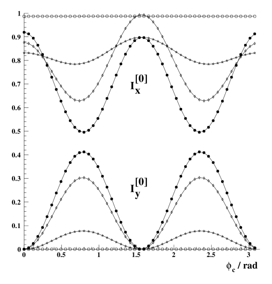
Figure 2: Intensity of the specular beams as function of the optical axis azimuth for various quartz plates: a tenth order quarter wave plate (full dots), 0.562 mm thickness (open dots), 5 mm thickness (diamonds) and a tenth order plate thickness but with the optical axis polar angle fixed to $\theta_{c}=\pi/4$ (stars). The upper set of curves represents the intensities $I^{[0]}_{x}$ and the lower set of curves $I^{[0]}_{y}$.

The results for the first order contributions $I_{x}^{[1]}$ and $I_{y}^{[1]}$ are shown in figures 3,4.

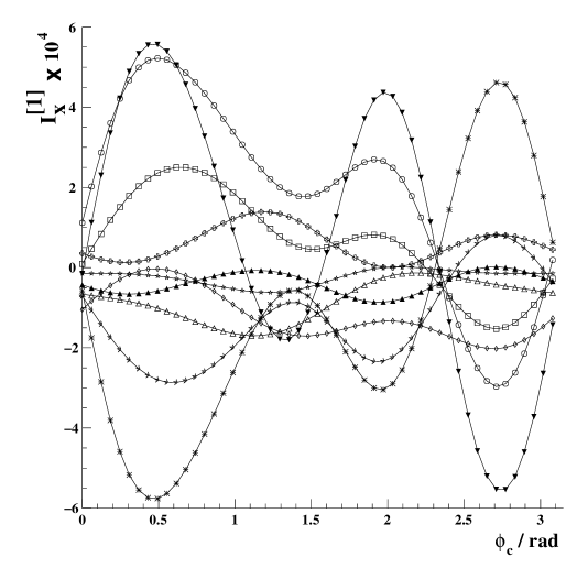
Figure 3: Interference between the specular and scattered transmitted fields $I^{[1]}_{x}$ as function of the optical axis azimuth. The plate is a tenth order quarter wave plate and the beam waist is $w_{0}=100\,\mu$m. Different symbols correspond to different random generated surface profiles.

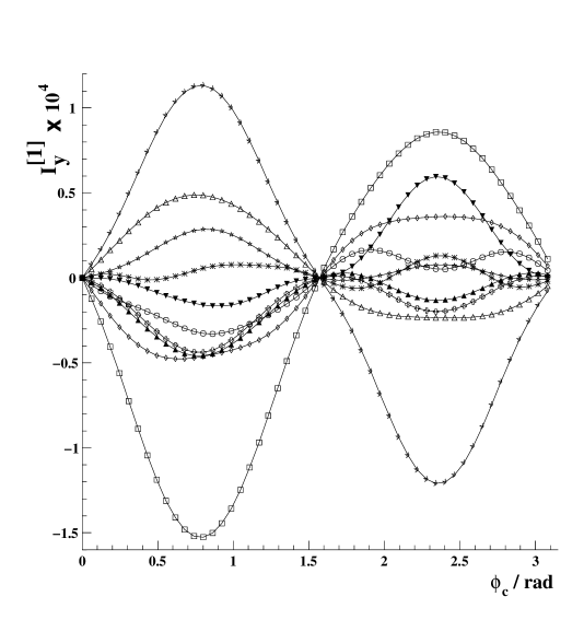
Figure 4: Interference between the specular and scattered transmitted fields $I^{[1]}_{y}$ as function of the optical axis azimuth. The plate is a tenth order quarter wave plate and the beam waist is $w_{0}=100\,\mu$m. Different symbols correspond to different random generated surface profiles.

Each curve of these plots corresponds to different surface profiles. Considering one given profile, one can notice that: the size of the specular-scattered interference strongly depends on the surface profile and can reach the per mill level of the zero order contribution, its sign changes with $\phi_{c}$ and its shape is not regular with $\phi_{c}$. The change of sign is expected since the intensity averaged over a large number of profiles obviously vanishes. The erratic shape is also expected since the fields change with $\phi_{c}$ and so do the Fourier transforms as the one of equation (23).

The second order contribution (calculated from equation (26)) is six order of magnitude smaller that the zero order contribution. However, we do not show any results since our second order calculation is not complete concerning the specular angular range.

Large differences are indeed observed when the plate thickness is changed. The specular-scattered interference contributions are computed for $a=0.562$ mm as in [8] (i.e. $(8+10^{-3})\times 2\pi$ retardation plate with our choice for the optical indices) and $a=5$ mm as in [7] (i.e. $(71+0.18)\times 2\pi$ retardation plate), and still with $\theta_{c}=\pi/2$. They are compared to the values obtained with the tenth order quarter wave plate and the same surface profiles.

The results are presented in figures 5,6. $I_{x}^{[1]}$ and $I_{y}^{[1]}$ scale with $I_{x}^{[0]}$ and $I_{y}^{[0]}$ (see figure 2). In particular, the oscillations of $I_{x}^{[1]}$ are dumped when $I_{x}^{[0]}$ gets flat (i.e. for the almost zero retardation plate $a=0.562$ mm).

To investigate the dependence of equations (19,14) on the optical axis polar angle $\theta_{c}$, the calculations were performed fixing $\theta_{c}=\pi/4$ for the plate thickness $a=0.720\,$mm. Here again the variations are noticeable (see figures 5 and 6).

Looking at figures 4 and 6, one can remark that $I_{y}^{[1]}$ tends to be of opposite sign in the regions $0<\phi_{c}<\pi/2$ and $\pi/2<\phi_{c}<\pi$. But this is not a general rule as it seems to come out from experiments [8, 7]. One can also observe two fix points at $\phi_{c}=0$ and $\pi/2$ on figures 4 and 6. $I_{y}^{[1]}$ being the interference between the scattered field and the zero order field, these fix points correspond to the zeros of the zero order field (see $I_{y}^{[0]}$ on figure 2). This is not the case for the second order term of equation (26) which is of the order of $10^{-6}$ and therefore dominates around $\phi_{c}=0,\pi/2$ (here the missing term of equation (26) is not relevant since it describes the interference between the specular and the second order scattered fields). However, the dispersion of $I_{y}^{[1]}$ around zero for $\phi_{c}=0,\pi/2$ (not visible on these figures) defers very slightly from zero, it is of the order of $10^{-10}$ for $w_{0}=100\,\mu$m and $\approx 10^{-8}$ for $w_{0}=25\,\mu$m. This is a cross-polarisation effect, i.e. this is due to the matrix $M_{3\times 3}$ in equations (20-22).

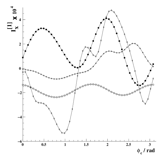
Figure 5: Interference between the specular and scattered transmitted fields $I^{[1]}_{x}$ as function of the optical axis azimuth for: a tenth order quarter wave plate (full dots), 0.562 mm thickness (open dots), 5 mm thickness plate (diamonds) and a tenth order plate thickness but with the optical axis polar angle fixed to $\theta_{c}=\pi/4$ (stars). The surface profiles are the same for the four curves.

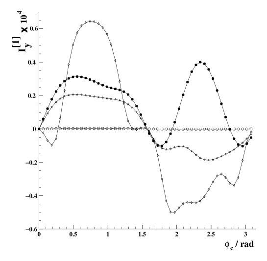
Figure 6: Same as figure 5 but for $I^{[1]}_{y}$.

The numerical results presented here are rather independent of the choice for the PSD2 provided a quartz plate of optical grade is considered. It is indeed experimentally demonstrated [14, 20, 31, 32, 33] that the PSDs of optical element’s surface have an inverse-power-low (or Fractal-like) behaviour. Therefore, various smooth mathematical representations of the PSD (see [34, 35] for examples) are reducible to equation (27) as it is justified in [31].

As a concluding remark, we point out that three important dimensionless parameters $\omega_{0}/l$, $\sigma/\lambda$ and $l/\lambda$ have been encountered in our calculations ($\omega_{0}/\lambda$ describes the cross-polarisation effects discussed above and is therefore not relevant here).

As mentioned in section 2, the validity of the perturbation treatment depends on $\sigma/\lambda$ and $l/\lambda$. Using the first order perturbation theory, the severe conditions $\sigma/\lambda\ll 1$ and $l/\lambda\simeq 1$ must hold[15]. They are fortunately fulfilled by optical grade quartz plates. To study the influence of the correlation length $l$, we changed the value of $l$ to $0.7\mu$m and $2\mu$m and we observed no significant qualitative differences with respect to the results described above.

As for the last dimensionless parameter $\omega_{0}/l$, we already mentioned that when $\omega_{0}/l\rightarrow\infty$ the usual result for plane waves is recovered (i.e. the specular-scattered interference term vanishes) although, with regard to the cut-off parameter $K_{min}$, this limit seems to be idealistic for a finite size quartz plate. To get an idea of the influence of $w_{0}$, we increased it to $200\mu$m and here again, no significant differences were observed. Much larger values for $w_{0}$ could not be tried, keeping a reasonable correlation length, because of the computer memory limitation. Finally let us mention that the other limit $\omega_{0}\ll l$ corresponds to the scattering by gratings [36]. In this limit the specular-scattered interference term vanishes since the diffusion occurs at large angle with respect to the specular beam direction.

4 Conclusion

We have computed, in the leading order perturbation theory, the effect of surfaces roughness on uniaxial platelets transmittance. Taking into account the Gaussian nature of laser beams we showed that the interference between the specular and scattered fields contributes to the intensity measurement performed in the specular region.

This contribution is of first order in the ratio of the root mean square roughness over the laser wavelength $\sigma/\lambda$. It depends strongly on the plate surfaces profiles and on the crystal optical properties, orientation of the optical axis, thickness and optical indices (i.e. temperature). It is therefore useless to implement the roughness calculation in a HAUP type of fitting procedure (in addition, the numerical calculation are computer time consuming).

In view of our numerical results, it is most likely that simple overlayer models [8] cannot describe accurately the dynamical properties of our main formula equations (14,19). Nevertheless, we point out that, because of the random property of the specular-scattered interference term, a simple way to avoid it is to perform a series of measurements at different locations on the plate and then to average the results. Although this procedure would increase the uncertainty on the determination of crystal optical parameters, it should however decrease the systematic bias. The determination of the plate thickness in situ could be done by varying the laser incident angle (i.e. by tilting the plate) [37].

Acknowledgement

I would like to thank J.P. Maillet for suggestions and enlightening discussions. I would also like to thank M.A. Bizouard for helpful discussions and F. Marechal for careful reading.

References

• [1] J. Kobayashi and Y. Uesu, “A new optical method and apparatus “HAUP” for measuring simultaneously optical activity and birefringence of crystals. I. Principle and construction ”, J. Appl. Cryst. 16, 204-211 (1983).
• [2] J.R.L. Moxon, A.R. Renshaw and I.J. Tebbutt, “The simultaneous measurement of optical activity and circular dichroism in birefringent linearly dichroic crystal sections: II. Description of apparatus and results for quartz, nickel sulphate hexahydrate and benzil”, J. Phys. D: Appl. Phys. 24, 1187-1192 (1991).
• [3] J. Ortega, J. Etxebarria, J. Zubillaga, T. Breczewski and M.J. Tello, “Lack of optical activity in the incommensurate phases of Rb2ZnBr4 and [N(CH3)4]2CuCl4”, Phys. Rev. B 45, 5155-5162 (1992).
• [4] C. Hernández-Rodríguez and P. Gómez-Garrido, “Optical anisotropy of quartz in the presence of temperature-dependent multiple reflections using a high-accuracy universal polarimeter”, J. Phys. D: Appl. Phys. 33, 2985-2994 (2000).
• [5] J.R.L. Moxon and R. Renshaw, “The simultaneous measurement of optical activity and circular dichroism in birefringent linearly dichroic crystal sections: I. Introduction and description of the method”, J. Phys.: Condens. Matter 2, 6807-6836 (1990).
• [6] M. Kremers and H. Meekes, “Interpretation of HAUP measurements: a study of the systematic errors”, J. Phys. D: Appl. Phys. 28, 1195-1211 (1995).
• [7] J. Simon, J. Weber and H-G Unruh, “Some new aspects about the elimination of systematical errors in HAUP measurements”, J. Phys. D: Appl. Phys. 30, 676-682 (1997).
• [8] C.L. Folcia, J. Ortega and J. Etxebarria, “Study of the systematic errors in HAUP measurements”, J. Phys. D: Appl. Phys. 32, 2266-2277 (1999).
• [9] F.G. Bass and I.M. Fuks, Wave scattering from statistically rough surfaces (Pergamon, Oxford, 1979).
• [10] J.A. Ogilvy, Theory of wave scattering from random rough surfaces (IOP Publishing Ltd, London, 1991).
• [11] Siegman A E 1986 Lasers ( Sausalito, California: University Science Books)
• [12] S. F. Nee,“Polarisation of specular reflection and near-specular scattering by rough surface”, Appl. Opt. 35, 3570-3582 (1996).
• [13] J. Brossel, “Multiple-beam localized fringes: Part I.- Intensity distribution and localization”, Proc. Phys. Soc. 59, 224-242 (1947)
• [14] A. Dupparé, J. Ferre-Borrull, S. Gleich, G. Notni, J. Steinert, and J.M. Bennett, “Surface characterization techniques for determining the root-mean-square roughness and power spectral densities of optical components”, Appl. Opt. 41, 154-171 (2002).
• [15] E.I. Thorsos and D.R. Jackson, “The validity of the perturbation approximation for rough surface scattering using a Gaussian roughness spectrum”, J. Acoust. Soc. Am. 86, 261-277 (1989).
• [16] W.L. Mochàn and R.G. Barrera, “Electromagnetic response of systems with spatial fluctuations. II Applications” Phys. Rev. B 32, 4989-5001 (1985).
• [17] N.R. Hill, “Integral-equation perturbative approach to optical scattering from rough surfaces”, Phys. Rev. B 24, 7112-7120 (1981).
• [18] V. Celli, T.T. Ong and P. Tran, “Light scattering from a random orientated anisotropic layer on a rough surface”, J. Opt. Soc. Am. A 11, 716-722 (1994).
• [19] R.A. Depine and M.E. Inchaussandague, “Corrugated diffraction gratings in uniaxial crystals”, J. Opt. Soc. Am. A 11, 173-180 (1994).
• [20] J.M. Bennett and L. Mattson, Introduction to surface roughness and scattering, (Opt. Soc. Am., Washington D.C., second edition 1999).
• [21] D.L. Mills and A.A. Maradudin, “Surface roughness and the optical properties of a semi-infinite material; the effect of a dielectric overlayer”, Phys. rev. B 12, 2943-2958 (1975).
• [22] B. Friedman, Principles and techniques of applied mathematics (Wiley, New-York, 1960). See Chap. 3.
• [23] A.A. Maradudin and D.L. Mills, “Scattering and absorption of electromagnetic radiation by semi-infinite medium in the presence of surface roughness”, Phys. Rev. B 11, 1392-1415 (1975).
• [24] P. Bousquet, F. Flory and P. Roche, “Scattering from multilayer thin films: theory and experiment”, J. Opt. Soc. Am. 71, 1115-1123 (1981).
• [25] D.L. Mills, “Attenuation of surface polaritons by surface roughness”, Phys. Rev. B 10, 4036-4046 (1975).
• [26] A.A. Maradudin and W. Zierau, “Effect of surface roughness on the surface-polariton dispertion relation”, Phys. Rev. B 14, 484-499 (1976).
• [27] F. Zomer, “Transmission and reflexion of Gaussian beams by anisotropic parallel plates”, J. Opt. Soc. Am. A. 20, 172-182 (2003).
• [28] N. Mukunda, R. Simon and E.C.G. Sudarshan, “Paraxial-wave optics and relativistic front description. II. The vector theory”, Phys. Rev. A 28, 2933-2942 (1983).
• [29] P. Yeh, “Electromagnetic propagation in birefringent media”, J. Opt. Soc. Am. 69, 742-756 (1979).
• [30] V.V. Azarova et al., “Measuring the roughness of high-precision quartz substrates and laser mirrors by angle resolved scattering”, J. Opt. Technol. 69, 125-128 (2002).
• [31] E.L. Church and P.Z. Takacs, “The optimal estimation of finish parameters”, in Optical Scatter: Applications, Measurements and Theory, J.C. Stover, ed., Proc. Soc. Photo-Opt. Instrum. Eng. 1530, 71-78 (1991).
• [32] E.L. Church, “Fractal surface finish”, Appl. Opt. 27, 1518-1526 (1988).
• [33] E. Marx, I.J. Malik, Y.E. Strausser, T. Bristow, N. Poduje and J.C. Stover, “Power spectral densities: a multiple technique study of different Si wafer surfaces”, J. Vac. Sci. Technol. B 20, 31-41 (2002).
• [34] J.M. Elson and J.M. Bennett, “Relation between the angular dependence of scattering and the statistical properties of optical surfaces”, J. Opt. Soc. Am. 69, 31-47 (1979).
• [35] G. Rasigni, F. Varnier, M. Rasigni, J.P. Palmari and A. Liebaria, “Spectral-density function of the surface roughness for polished optical surfaces”, J. Opt. Soc. Am. 73, 1235-1239 (1983).
• [36] G. Tayeb, “Sur l’étude numérique de réseaux de diffraction constitués de matériaux anisotropes”, C. R. Acad. Sci. Paris 307, 1501-1504 (1988).
• [37] J. Poirson et al., “Jones matrix of a quarter-wave plate for Gaussian beams”, Appl. Opt. 34, 6806-6818 (1995).