The potential of the ground state of NaRb

Abstract

The X${}^{1}\Sigma^{+}$ state of NaRb was studied by Fourier transform spectroscopy. An accurate potential energy curve was derived from more than 8800 transitions in isotopomers ²³Na⁸⁵Rb and ²³Na⁸⁷Rb. This potential reproduces the experimental observations within their uncertainties of 0.003 cm^-1 to 0.007 cm^-1. The outer classical turning point of the last observed energy level ($v^{\prime\prime}=76$, $J^{\prime\prime}=27$) lies at $\approx 12.4$ Å, leading to a energy of 4.5 cm^-1 below the ground state asymptote.

I Introduction

The heteronuclear alkali dimers attract interest of both experimental and theoretical researchers involved in collision dynamics, photoassociative spectroscopy, laser cooling and trapping of alkali atoms Shaffer:99 ; Ferrari:02 ; Hadzibabic:02 ; Weiss:03 . Special interest is put on the study of the ground states and especially near the atomic asymptote, since the precise knowledge of the long-range interactions between two different types of alkali atoms is necessary for understanding and realization of such cold collision processes as sympathetic cooling, formation of two species BEC (TBEC) and ultracold heteronuclear molecules.

Although the NaRb molecule is one of the promising candidates for TBEC Weiss:03 , the experimental information on the ground singlet state is still limited.

Accurate term values of the X${}^{1}\Sigma^{+}$ state were determined by the Doppler-free polarization spectroscopy Wang2:91 . They cover a range of low vibrational quantum numbers $v^{\prime\prime}\in[0,6]$ with limited sets of rotational quantum numbers (e.g. $J^{\prime\prime}\in[1,80]$ for $v^{\prime\prime}=0$ and $J^{\prime\prime}\in[18,36]$ for $v^{\prime\prime}=6$). Later Kasahara et al. Kasahara:96 extended the range of $v^{\prime\prime}$ up to $v^{\prime\prime}=30$, but only for $J^{\prime\prime}=10,12$. On the other hand the recent experiment by the Riga group Docenko:02 collected about 300 transition frequencies to energy levels with a much wider spectrum of vibrational and rotational quantum numbers ($v^{\prime\prime}\in[15,76]$, $J^{\prime\prime}\in[12,64]$) but with relatively moderate accuracy ( 0.1 cm^-1 ). A hybrid potential for the NaRb ground state based on extrapolation between regions determined from the early experimental data Wang2:91 ; Kasahara:96 and the theoretical dispersion coefficients from Ref. Marinescu:99 was constructed by Zemke et al. Zemke:NaRb giving an improved estimate on the dissociation energy of the ground state - $D_{\mathrm{e}}=5030.75$ cm^-1.

On the theoretical side two papers have recently appeared: by Korek et al. Korek:00 and by Zaitsevskii et al. Zaitsevskii:01 . In both of them theoretical potential energy curves for the ground and several excited states are given. Results from Ref. Korek:00 on selected low electronic states are shown also in Figure 1, which will help in following the electronic assignment of the new observations, reported below.

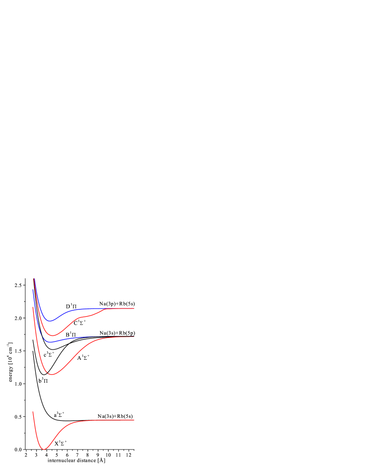
Figure 1: Selected low singlet and triplet electronic states in NaRb according to Ref. Korek:00 .

The goal of the present investigation is to study extensively the ground electronic state X${}^{1}\Sigma^{+}$ of the NaRb molecule. We chose the Fourier transform spectroscopy which is able to provide abundant and precise spectroscopic data, needed for construction of an accurate potential energy curve. In addition, this study is considered as the necessary background for further investigations of this molecule at long internuclear distances required for modeling cold collisions at 1mK and below.

II Experiment

The NaRb molecules were produced in a single section heat-pipe oven similar to that described in Ref. Allard:02 by heating 5 g of Na (purity 99.95 %) and 10 g of Rb (purity 99.75 %, natural isotopic composition) from Alfa Aesar. The oven was operated at temperatures between 560 K and 600 K and typically with 2 mbar of Ar as buffer gas. At these conditions apart from the atomic vapors all three types of molecules are formed - Na₂, Rb₂ and NaRb. This mixture was illuminated by three different laser sources: a single mode, frequency doubled Nd:YAG laser, Ar⁺ ion laser and Rhodamine 6G dye laser. Their wavelengths fall in a spectral window with weak absorption of Rb₂. Setting the working temperatures as low as possible we reduced the density of the Na₂ molecules reaching a relatively intense NaRb spectra free of Na₂ emission. The heat pipe oven was in operation more than 60 hours without refilling and at the end of the experiment was still in good working condition.

The fluorescence from the oven was collected in the direction opposite to the propagation of the laser beam and then focused into the input aperture of Bruker IFS 120 HR Fourier transform spectrometer. The signal was detected with a Hamamatsu R928 photomultiplier tube or a silicon diode. The scanning path of the spectrometer was set to reach a typical resolution of 0.0115 cm^-1 $\div$ 0.03 cm^-1 and the number of scans for averaging varied between 10 and 20. In order to avoid the illumination of the detector by the He-Ne laser, used for calibration of the spectrometer, a notch filter with 8 nm FWHM was introduced. For better signal-to-noise ratio some spectra were recorded by limiting the desired spectral window with colored glass or interference filters.

The single mode, frequency doubled Nd:YAG laser with a typical output power of 70 mW at 532.1 nm excited the C${}^{1}\Sigma^{+}\leftarrow$ X${}^{1}\Sigma^{+}$ and D${}^{1}\Pi\leftarrow$ X${}^{1}\Sigma^{+}$ systems of NaRb, compare Fig. 1. The frequency was varied between 18787.25 cm^-1 and 18788.44 cm^-1 and spectra were recorded at frequencies which excite strong fluorescence.

The Ar⁺ ion laser was operated both in single (typical power 100$\div$500 mW) and multi mode (typical power 0.5$\div$3 W) regimes. The 514.5 nm, 501.7 nm, 496.5 nm, 488.0 nm and 476.5 nm Ar⁺ ion laser lines induced fluorescence mainly due to the D${}^{1}\Pi\leftarrow$ X${}^{1}\Sigma^{+}$ system of NaRb. The Na₂ B${}^{1}\Pi_{\mathrm{u}}\rightarrow$ X${}^{1}\Sigma^{+}_{\mathrm{g}}$ band was also observed, especially exciting with the bluer Ar⁺ laser lines, but its intensity was reduced by decreasing the working temperature down to 560 K. Along with the D $\leftarrow$ X system, the 514.5 nm line excites also transitions in the C${}^{1}\Sigma^{+}\leftarrow$ X${}^{1}\Sigma^{+}$ system of NaRb Docenko:02 . The special form of potential energy curve of the C${}^{1}\Sigma^{+}$ state Korek:00 results in favorable Franck-Condon factors for transitions from some C state levels both to low and high lying energy levels of the ground state. Such C state levels are excited by the 514.5 nm line and the green florescence of the D $\leftarrow$ X system is accompanied by a red fluorescence due to C $\leftarrow$ X transitions, which reach $v^{\prime\prime}=76$ of the ground state (Fig. 2).

In order to bring the frequency of the single mode Ar⁺ laser exactly in resonance with desired transitions we did the following. As a first step we recorded the LIF for a given frequency simultaneously with the Fourier spectrometer and a GCA/McPherson Instruments scanning monochromator (1m focal length). The high resolution Fourier spectrum helped us to assign unambiguously the record of the monochromator. Then we set the monochromator on a strong and pronounced line of the progression of interest and we tuned the Ar⁺ laser frequency until the maximum signal on the monochromator was reached. The frequency stability of the laser with a temperature stabilized intracavity etalon was sufficient in order to perform 10 to 20 scans with the Fourier spectrometer.

Figure 2: The vibrational progression up to $v^{\prime\prime}=76$ in Na⁸⁵Rb excited by a single mode Ar⁺ laser. Lines not indicated are also assigned.

The Rhodamine 6G laser excites the B${}^{1}\Pi\leftarrow$ X${}^{1}\Sigma^{+}$ transition and also weak transitions in the C${}^{1}\Sigma^{+}\leftarrow$ X${}^{1}\Sigma^{+}$ system and was used for two reasons. The first was to enrich the information on the ground state levels with intermediate vibrational quantum numbers because of the gap between the levels from the D${}^{1}\Pi\leftarrow$ X${}^{1}\Sigma^{+}$ system (mainly with low $v^{\prime\prime}$) and those from the C${}^{1}\Sigma^{+}\leftarrow$ X${}^{1}\Sigma^{+}$ system (mainly with high $v^{\prime\prime}$). Secondly, we wanted to excite levels of the B state with significant triplet admixture due to perturbations from the neighboring b${}^{3}\Pi$ and c${}^{3}\Sigma^{+}$ states Wang2:91 ; Wang:92 . Indeed, scanning the frequency of the dye laser from 16729 cm^-1 to 16965 cm^-1 we encountered a large number of excitations where a second fluorescence band around 12000 cm^-1 appeared along with the B $\leftarrow$ X system (see Fig. 3). The analysis of this band (a report is in preparation) confirmed that we have observed transitions to the ground triplet state a${}^{3}\Sigma^{+}$.

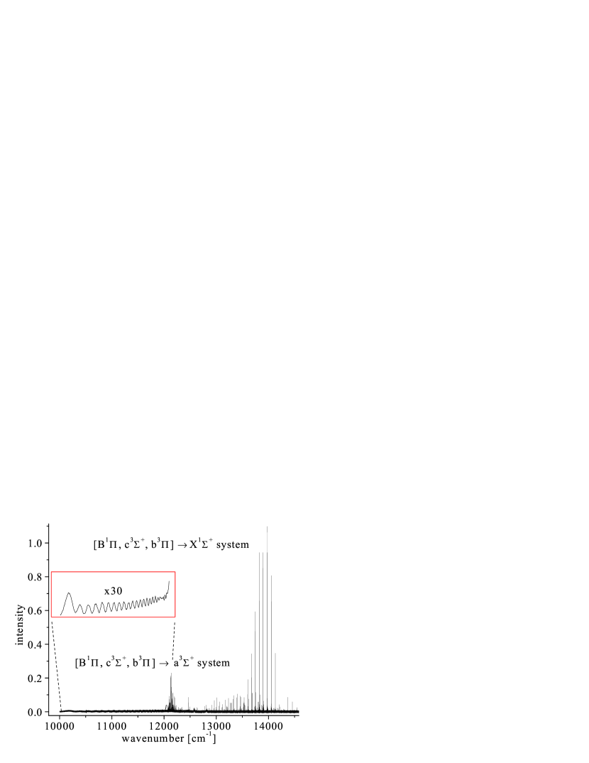
Figure 3: The [B${}^{1}\Pi$, b${}^{3}\Pi$, c${}^{3}\Sigma^{+}$]-X${}^{1}\Sigma^{+}$ and [B${}^{1}\Pi$, b${}^{3}\Pi$, c${}^{3}\Sigma^{+}$]-a${}^{3}\Sigma^{+}$ bands of NaRb excited by a single mode Rhodamine 6G laser. The insert shows the continuum due to the bound-free emission to the repulsive wall of the a${}^{3}\Sigma^{+}$ state.

All transitions excited in Na⁸⁵Rb and Na⁸⁷Rb by the single mode Nd:YAG and Rhodamine 6G lasers and by the Ar⁺ laser in single- and multi mode, assigned and used in this analysis are listed in Table 1 of the supplementary material (EPAPS No. ….).

III Analysis

The assignment of the recorded spectra was simplified by the published potential energy curve in Ref. Docenko:02 . After we identified the strongest progressions, which were already observed in previous studies Takahashi:81 ; Nikolayeva:00 ; Zaitsevskii:01 ; Docenko:02 , a new potential was fitted. This preliminary potential was further improved filling additionally collected experimental data; this sequential procedure allows continuous checking of the assignment, especially for high $J^{\prime\prime}$ and in cases of large gaps in $v^{\prime\prime}$. The total data set (Fig. 4) consists of more than 6150 transitions in Na⁸⁵Rb and 2650 in Na⁸⁷Rb given in Table 2 of the supplementary material (EPAPS No…..).

Figure 4: The range of vibrational and rotational quantum numbers of the observed ground state energy levels in Na⁸⁵Rb and Na⁸⁷Rb

For fitting the experimental data we used the approach adopted in Ref. Allard:02 . In order to exclude any fitting parameters concerning the excited states, we fitted the ground state potential directly to the observed differences between ground state levels. In our case of 8800 transitions we selected about 43300 differences for representing the different cases of vibrational intervals (for details see also Allard:02 ). The uncertainties of the differences were estimated taking into account the instrumental accuracy and resolution, and the signal-to-noise ratio for both transitions forming the difference. The uncertainty of strong lines was set to 0.002 $\div$ 0.003 cm^-1 increasing to 0.007 cm^-1 for weaker ones with SNR $\approx 2$. Differences which were measured several times were averaged with weighting factors determined from their uncertainties.

As already discussed in Allard:02 , for our experimental set up a fluorescence progression excited by a single mode laser will be shifted in frequency if the laser is not tuned to the center of the Doppler profile. This problem is partially overcome by fitting differences instead of transition frequencies. Nevertheless there can be still a residual shift of the differences due to the frequency dependence of the Doppler shift. For example if the laser frequency around 20000 cm^-1 is detuned from the line center by one Doppler width (about 0.03 cm^-1 for NaRb at 600 K) the difference between two transitions $\nu_{1}$ and $\nu_{2}$ separated by $\nu_{1}-\nu_{2}$= 4000 cm^-1 will be shifted from the “true” one by 0.006 cm^-1. This shift is comparable with the typically expected uncertainty ($\approx 0.004$ cm^-1) but it cannot be determined in our experiment. Therefore, initially we did not correct the uncertainties of the large differences (a possible solution could be to increase the uncertainty of the difference $\nu_{1}-\nu_{2}$ proportionally to the ratio $(\nu_{1}-\nu_{2})/\nu_{1}$). Large differences however were checked carefully during the fitting procedure and finally no need for such correction was found.

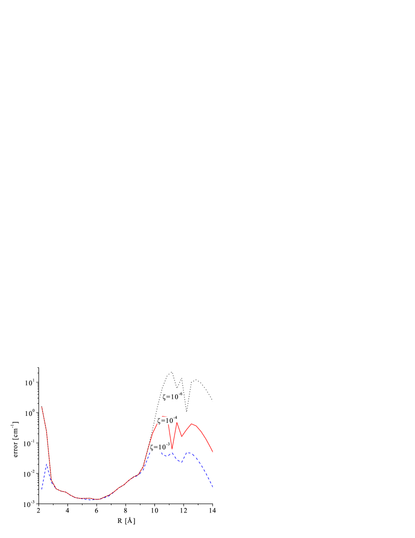
Figure 5: The derived standard deviation (in logarithmic scale) of the points of the pointwise potential curve for three different values of the singularity parameter $\zeta$ (for details see Ref. Allard:02 ).

IV Construction of PEC

The ground singlet states of both isotopomers of NaRb are described in the adiabatic approximation with a single potential energy curve. The potential was constructed as a set of points $\{R_{i},U(R_{i})\}$ (see Ref. ipaasen ) connected with cubic spline function. The pointwise representation of the potential, however, is not convenient for long internuclear distances. On the other hand, in order to ensure proper boundary conditions for solving the Schrödinger equation for high vibrational energy levels, distances up to $R\approx 20$ Å are needed. Therefore for $R\geq R_{\mathrm{out}}$ we adopted the usual dispersion form:

$$U(R)=D_{e}-C_{6}R^{-6}-C_{8}R^{-8}-C_{10}R^{-10}\mbox{ ,}$$ (1)

with coefficients $C_{6},C_{8}$ taken from Ref. Derevianko:01a ; Porsev:03 . The connecting point $R_{\mathrm{out}}$ and the parameters $D_{e}$ and $C_{10}$ were varied in order to ensure a smooth connection with the pointwise potential as follows. Initially, the PEC was constructed in a pointwise form up to 16 Å. After each fitting iteration $D_{e}$ and $C_{10}$ were adjusted to fit the shape of the pointwise potential between 13.0 Å and 16.0 Å to the analytic formula (1). The crossing point of the pointwise and the long range curves was taken as $R_{\mathrm{out}}$. Since the experimental data are almost insensitive to details of the potential shape in this region, we found this procedure sufficient and did not fit the long range parameters directly to the experimental data. Once the final form of the PEC was achieved, we found that it is possible to extend the validity of the long range expression down to approximately 11.8 Å. At the same time the quality of the derived potential did not change if the analytic formula (1) was fitted to the shape of the pointwise potential between 11.8 Å and 13.24 Å. A discussion on the advantage of using this matching procedure can be found in Ref. MC:03 .

The final set of potential parameters consists of 51 points. In order to calculate the value of the potential for $R<R_{\mathrm{out}}$ a natural cubic spline Numer through all 51 points and for $R\geq R_{\mathrm{out}}$ the long range expression (1) should be used with parameters listed in Table 1. This final PEC gives a standard deviation of $\sigma=0.0031$ cm^-1 and a normalized standard deviation of $\bar{\sigma}=0.70$ showing the internal consistency of the data set and the quality of the derived potential.

Table 1: Pointwise representation of the potential energy curve for the X${}^{1}\Sigma^{+}$ state of NaRb.

R [Å]	U [cm-1]	R [Å]	U [cm-1]
2.101916	21110.5539	5.167536	2866.7126
2.200000	16374.1819	5.328985	3174.1150
2.298084	12751.3674	5.490435	3450.2078
2.396168	9944.6386	5.651884	3694.1882
2.494252	7761.9582	5.813333	3906.7423
2.592337	5992.3235	6.065085	4179.8842
2.690421	4637.9707	6.253898	4343.3002
2.788505	3543.2165	6.442712	4476.4609
2.886589	2638.9307	6.631525	4584.0755
2.984673	1900.4037	6.820339	4670.5331
3.082757	1308.0797	7.009152	4739.7196
3.180841	845.5522	7.197966	4794.9580
3.278926	498.1298	7.386780	4839.0226
3.377010	252.2899	7.556326	4870.9517
3.475094	95.41660	7.783673	4904.8112
3.573178	15.73046	8.098462	4939.0358
3.671262	2.3375	8.384103	4961.0335
3.792152	62.2402	8.669744	4977.0314
3.933165	217.7034	9.014483	4990.8655
4.074177	443.0825	9.398621	5001.4491
4.215190	718.3282	9.722105	5007.8576
4.360290	1035.8028	10.201818	5014.3657
4.521739	1411.4474	11.214546	5022.0531
4.683188	1794.2206	12.227273	5025.7686
4.844638	2170.6796	13.240000	5027.9612
5.006087	2530.6262
$D^{\mathrm{X}}_{\mathrm{e}}$=5030.8480 cm-1
$R_{\mathrm{out}}$=12.090520 Å		$C_{8}$=3.590$\cdot 10^{8}$ cm-1Å8
$C_{6}$=1.293$\cdot 10^{7}$ cm-1Å6		$C_{10}$=3.539$\cdot 10^{10}$ cm-1Å10

In order to find the region where the PEC is unambiguously characterized by the experimental data we analyzed the uncertainty of the fitting parameters as described in detail in Ref. Li2F:00 ; Allard:02 . By minimizing the merit function $\chi^{2}$ using the Singular Value Decomposition (SVD) method Wilkinson:SVD ; Numer it is possible to determine the parameters on which $\chi^{2}$ and consequently the quality of the fit depend only weakly. The fitting parameters in our case are the values of the potential itself in a preset grid of points. In Fig. 5 the uncertainties of the fitted potential for intermediate internuclear distances are presented for three different values of the singularity parameter $\zeta$ (see Li2F:00 ). Although the outer classical turning point of the last observed energy level ($v^{\prime\prime}=76$, $J^{\prime\prime}=27$) is 12.4 Å  we see that the shape of the potential energy curve is unambiguously fixed (within the experimental uncertainty) approximately only between 3.0 Å and 9.8 Å since the uncertainties there almost do not depend on $\zeta$. Therefore, although the fitted potential energy curve describes all the experimental data up to $v^{\prime\prime}=76$, there is no rigorous way to estimate the uncertainty of its shape beyond 9.8 Å (see also Allard:02 ). The result of Fig. 5 might indicate that the correlation between the left (R $<$ 3Å) and right (R $>$ 9.8 Å) branch of the potential becomes significant. In this respect the reported potential in Table 1 for these regions is only one possibility which describes our observations within the error limits. From Table 1 we derive some parameters which will be useful when applying the potential for other calculations and spectroscopic studies. Their values are not rounded in order to keep consistency with the data from Table 1.

• equilibrium distance of the potential,
  $R_{e}=3.643415$ Å,

• position of the level with $v^{\prime\prime}=0$ and $J^{\prime\prime}=0$,
  $E_{00}=53.3117$ cm^-1 with respect to potential minimum,

• the dissociation energy of the ground state, calculated with respect to $E_{00}$,
  $D^{\mathrm{X}}_{0}$=4977.5363 cm^-1.

In Fig. 6 the potential energy curves published in Ref. Zemke:NaRb ; Docenko:02 are compared with the pointwise potential (PW) of this study. The reason for the difference between the PW potential and the Modified Lennard-Jones (MLJ) potential Docenko:02 around $R_{e}$ is probably that for the construction of the later potential the rotational quantum numbers for levels with $v^{\prime\prime}<30$ were limited only to the narrow interval from Kasahara:96 ($J^{\prime\prime}=10,12$). With such data set the rotational constant $B_{v}$ can be determined only with large uncertainty which corresponds to shifts of the whole potential along the internuclear axes which is clearly indicated in Fig. 6. As already discussed in Section I the hybrid potential from Ref. Zemke:NaRb was constructed using the whole range of available rotational quantum numbers from the literature (Wang2:91 ; Kasahara:96 ) and therefore the agreement with the present study around $R_{e}$ is much better. The deviations between the PW and the hybrid potential reaching 20 cm^-1 for intermediate internuclear distances are caused by the extrapolation between the theoretical long range part of the potential and the experimental short range part. In the same region the experimentally determined shape of the MLJ potential is in a much better agreement with the present study.

Since the primary data from Wang2:91 were not available to us, we were able to check our potential only against the data published in Kasahara:96 . Forming differences between transition frequencies exactly as for our LIF data we found an agreement with the differences predicted by the present PEC from Table 1 with a standard deviation of 0.0026 cm^-1, well within the expected experimental error of 100 MHz. Only two transitions ((12,11)-(17,10) and (12,11)-(19,10)) were excluded from this comparison since differences with them showed systematically large deviations reaching 0.01 cm^-1.

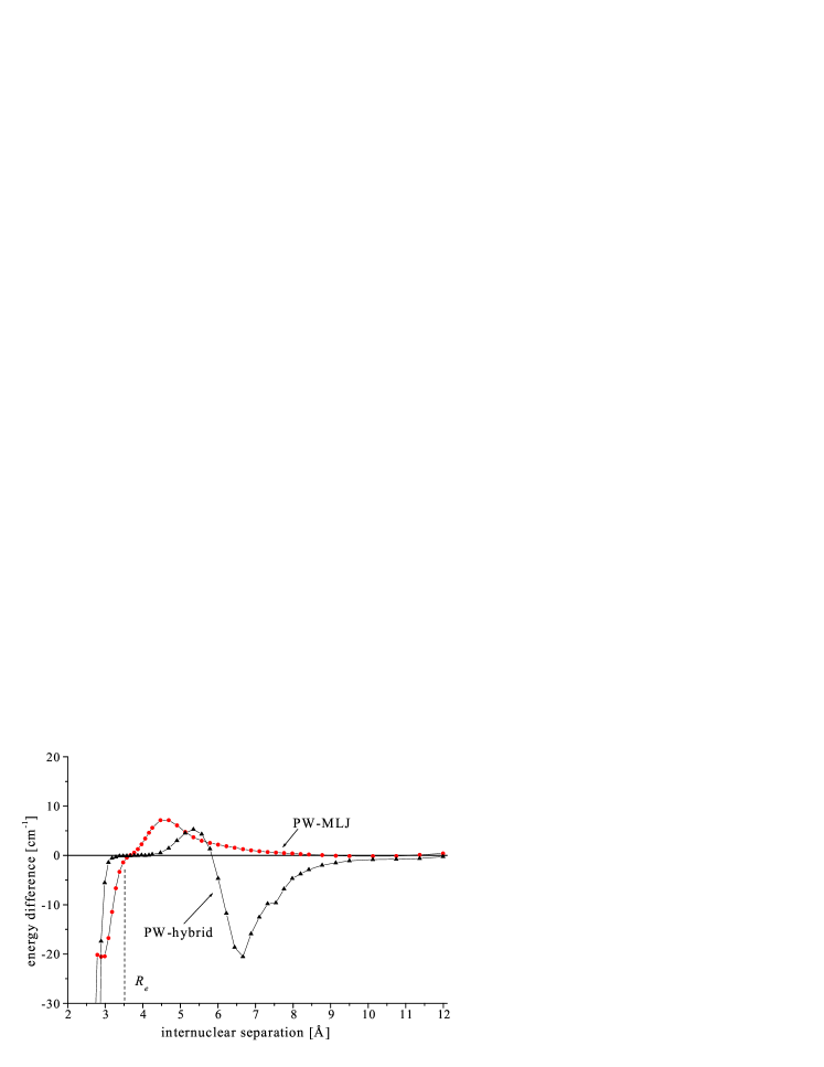
Figure 6: Differences between the pointwise representation of the NaRb ground state potential derived in this study (PW) and previous potentials energy curves from Ref. Zemke:NaRb (Hybrid), Ref. Docenko:02 (MLJ). The energy at the equilibrium point $R_{e}$ is set to zero for all potentials and used as a reference point.

In Table 2 a set of Dunham coefficients for ²³Na⁸⁵Rb is listed which describes the whole set of the measured differences for both isotopomers with a deviation of 0.0030 cm^-1 and a normalized standard deviation of 0.84. For calculating the eigenvalues for ²³Na⁸⁷Rb the usual scaling rules were used. The distribution of the indexes of the Dunham coefficients indicates that for description of such a large set of vibrational and rotational quantum numbers the parameters of the Dunahm expansion lose their original meaning of “spectroscopic constants”. The extremely small values of some coefficients ($\sim 10^{-40}$ cm^-1 !) indicate that they should be used with caution due to roundoff errors. At last, the extrapolation properties of such set of Dunham coefficients are doubtful. Therefore, we prefer to give the full description of the experimental data by a potential energy curve, which is obviously a much better physical model, and to present Dunham coefficients only for convenience since there are still applications where their use is easier and faster.

Table 2: Dunham coefficients for ²³Na⁸⁵Rb in cm^-1, derived from the experimental data with $v^{\prime\prime}\leq 76$ and $J^{\prime\prime}\leq 200$.

$i$

$k$

$Y_{ik}$

1	0	$106.8544964$
2	0	$-0.37984464$
3	0	$-7.703864$	$\times 10^{-4}$
5	0	$-5.390011$	$\times 10^{-7}$
7	0	$6.5551619$	$\times 10^{-10}$
9	0	$-1.9725192$	$\times 10^{-12}$
10	0	$9.9663375$	$\times 10^{-14}$
11	0	$-2.5123$	$\times 10^{-15}$
12	0	$3.7418$	$\times 10^{-17}$
13	0	$-3.33869$	$\times 10^{-19}$
14	0	$1.652$	$\times 10^{-21}$
15	0	$-3.48$	$\times 10^{-24}$
0	1	$7.019021$	$\times 10^{-2}$
1	1	$-2.943389$	$\times 10^{-4}$
2	1	$-1.699605$	$\times 10^{-6}$
4	1	$-1.474183$	$\times 10^{-9}$
6	1	$5.732233$	$\times 10^{-12}$
7	1	$-3.68622$	$\times 10^{-13}$
8	1	$1.031766$	$\times 10^{-14}$
9	1	$-1.2551$	$\times 10^{-16}$
11	1	$1.22142$	$\times 10^{-20}$
13	1	$-1.6097$	$\times 10^{-24}$
14	1	$9.446$	$\times 10^{-27}$
0	2	$-1.20357$	$\times 10^{-7}$
1	2	$-7.98199$	$\times 10^{-10}$
2	2	$-4.21837$	$\times 10^{-12}$
7	2	$-1.2888117$	$\times 10^{-17}$
8	2	$1.760426295$	$\times 10^{-18}$
9	2	$-1.17937534$	$\times 10^{-19}$
10	2	$4.906556$	$\times 10^{-21}$
11	2	$-1.3413739$	$\times 10^{-22}$
12	2	$2.3980927$	$\times 10^{-24}$
13	2	$-2.684354$	$\times 10^{-26}$
14	2	$1.70$	$\times 10^{-28}$
15	2	$-4.6349$	$\times 10^{-31}$
0	3	$1.4803$	$\times 10^{-13}$
1	3	$1.9481$	$\times 10^{-15}$
3	3	$-9.3543$	$\times 10^{-18}$
8	3	$7.87129$	$\times 10^{-24}$
9	3	$-6.789833$	$\times 10^{-25}$
10	3	$2.13759$	$\times 10^{-26}$
11	3	$-2.61852$	$\times 10^{-28}$
13	3	$1.974$	$\times 10^{-32}$
15	3	$-1.0266$	$\times 10^{-36}$
1	4	$-1.953$	$\times 10^{-20}$
2	4	$-1.906$	$\times 10^{-21}$
5	4	$1.11596$	$\times 10^{-24}$
6	4	$-7.344$	$\times 10^{-26}$
8	4	$7.4791$	$\times 10^{-29}$
10	4	$-6.261$	$\times 10^{-32}$
11	4	$8.982$	$\times 10^{-34}$
14	4	$-6.3065$	$\times 10^{-40}$
7	5	$-1.3005$	$\times 10^{-33}$

V Results and Discussion

In this paper a spectroscopic study of the NaRb ground state is presented. A variety of laser sources was used to excite several band systems in both isotopomers of the NaRb molecule and the induced fluorescence was analyzed with a high resolution Fourier transform spectrometer. More than 8800 transitions were identified resulting in a set of more than 4000 ground state energy levels with wide range of vibrational and rotational quantum numbers. An accurate potential energy curve was fitted to the experimental data reproducing differences between ground state energy levels with $\sigma=0.0031$ cm^-1 and $\bar{\sigma}=0.70$.

In order to check the consistency of the derived potential energy curve we performed additional fits in several different ways. Instead of fitting differences, we applied the commonly used approach of fitting directly transition frequencies, getting the term energies of the excited state levels as free parameters. In this case two representations of the potential were tried: a pointwise and an analytic form described in detail in Ref. Samuelis:00 . Both representations gave the same quality of the fit compared to the pointwise potential determined from differences and the potentials were practically identical in the studied range. Thus no additional parameters sets are given here in order to avoid the confusion of the reader what potential form should be preferred.

The classical turning point of the last observed energy level ($v^{\prime\prime}=76$, $J^{\prime\prime}=27$) is around 12.4 Å. Although this point lies beyond the Le Roy radius for the NaRb 3²S+5²S asymptote ($R_{\mathrm{LeRoy}}=11.2$ Å), the analysis of the PEC uncertainties indicates that with the present body of experimental data it is unsafe to determine $C_{6}$ and the other dispersion coefficients. For this reason the experimental PEC was smoothly connected to a long range potential formed by dispersion terms taken from the literature Derevianko:01a ; Porsev:03 . For better description of the near asymptotic region of the PEC transition frequencies to weakly bound energy levels are needed (see for example MC:03 ). Some improvement might be expected already from the combined analysis of the X${}^{1}\Sigma^{+}$ and a${}^{3}\Sigma^{+}$ states at long internuclear distances which is in progress.

Weiss et al. Weiss:03 applied the MLJ potential from Docenko:02 and extended it for $R>11$ Å  by the long range parameters from Marinescu:99 ; Derevianko:01a and the exchange interaction taken from Smirnov:65 to determine the singlet and triplet scattering lengths for 3²S Na + 5²S Rb. Using the newly derived potential for the inner part we constructed the full potential with the same long range parameters as in Weiss:03 and derived a singlet scattering length of +305a₀ ($a_{0}\approx 0.52918$ Å, the Bohr radius) for ²³Na⁸⁵Rb and +103a₀ for ²³Na⁸⁷Rb. These results do not agree with the ones from Ref. Weiss:03 : +167a₀ (+50a₀/-30a₀) for ²³Na⁸⁵Rb and 55a₀ (+3a₀/-3a₀) for ²³Na⁸⁷Rb. We used exactly the same approach for the long range as in Weiss:03 to see clearly the influence of the inner part of the potential. By the new values we will not claim that we have determined more realistic scattering lengths. Rather we want to point out that the existing data do not allow to specify the scattering length in an useful uncertainty interval. Note also that slight changes in the exchange energy still allow to alter the sign of the scattering length in ²³Na⁸⁵Rb. Thus energy levels closer to the asymptote ($<4.5$ cm^-1) must be studied.

VI Acknowledgments

This work is supported by DFG through SFB 407. The authors appreciate the assistance of M. Klug and Ch. Samuelis during the experiments. A.P. gratefully acknowledges the research stipend from the Alexander von Humboldt Foundation. O. D., M. T. and R. F. acknowledge the support by the University of Latvia, by the Latvian Science Council grant 01.0264, the Latvian Ministry of Education and Science (grant TOP 02-45) as well as by NATO SfP 978029 - Optical Field Mapping grant.

References

- (1) James P. Shaffer, Witek Chalupczak, and N. P. Bigelow. Phys. Rev. A 60, R3365 (1999).
- (2) G. Ferrari, M. Inguscio, W. Jastrzebski, G. Modugno, G. Roati and A. Simoni. Phys. Rev. Lett. 89, 53202 (2002).
- (3) Z. Hadzibabic, C. A. Stan, K. Dieckmann, S. Gupta, M. W. Zwierlein, A. Görlitz and W. Ketterle. Phys. Rev. Lett. 88, 160401 (2002).
- (4) S. B. Weiss, M. Bhattacharya and N. P. Bigelow. arXiv:physics/0303006 v1.
- (5) Y.-C. Wang, M. Kajitani, S. Kasahara, M. Baba K. Isikawa, and H. Katô. J. Chem. Phys. 95, 6229 (1991).
- (6) S. Kasahara, T. Ebi, M. Tanimura, H. Ikoma K. Matsubara, M. Baba, and H. Katô. J. Chem. Phys. 105, 1341 (1996).
- (7) O. Docenko, O. Nikolayeva, M. Tamanis, R. Ferber, E. A. Pazyuk and A. V. Stolyarov. Phys. Rev. A 66, 052508 (2002).
- (8) M. Marinescu and H. R. Sadeghpour. Phys. Rev. A 59, 390 (1999).
- (9) W. T. Zemke and W. C. Stwalley. J. Chem. Phys. 114, 10811 (2001).
- (10) M. Korek, A.R. Allouche, M. Kobeissi, A. Chaalan, M. Dagher, K. Fakherddin and M. Aubert-Frécon. Chem. Phys. 256, 1 (2000).
- (11) A. Zaitsevskii, S.O. Adamson, E.A. Pazyuk, A.V. Stolyarov, O. Nikolayeva, O. Docenko, I. Klincare, M. Auzinsh, M. Tamanis, R. Ferber and R. Cimiraglia. Phys. Rev. A 63, 052504 (2001).
- (12) O. Allard, A. Pashov, H. Knöckel and E. Tiemann. Phys. Rev. A 66, 42503 (2002).
- (13) Y.-C. Wang, K. Matsubara, and H. Katô. J. Chem. Phys. 97, 811 (1992).
- (14) N. Takahashi and H. Katô. J. Chem. Phys. 75, 4350 (1981).
- (15) O. Nikolayeva, I. Klincare, M. Auzinsh, M. Tamanis, R. Ferber, E. A. Pazyuk, A. V. Stolyarov, A. Zajtsevskii and R. Cimiraglia. J. Chem. Phys. 113, 4896 (2000).
- (16) A. Pashov, W. Jastrzȩbski, and P. Kowalczyk. Comput. Phys. Commun. 128, 622 (2000).
- (17) W. H. Press, S. A. Teukolski, W. T. Vetterling, and B. P. Flannery. Numerical Recipes in Fortran 77. Cambridge Unversity Press, 1992.
- (18) A. Dervianko, J. F. Babb and A. Dalgarno. Phys. Rev. A 63, 052704 (2001).
- (19) S. G. Porsev and A. Derevianko. J Chem. Phys. 119, 844 (2003).
- (20) O. Allard, C. Samuelis, A. Pashov, H. Knöckel and E. Tiemann. Eur. Phys. J. D 26, 155 (2003).
- (21) A. Pashov, W. Jastrzȩbski, and P. Kowalczyk. J. Chem. Phys. 113, 6624 (2000).
- (22) J. H. Wilkinson and C. Reinsch. Linear Algebra. Springer-Verlag, Berlin, 1971.
- (23) C. Samuelis, E. Tiesinga, T. Laue, M. Elbs, H. Knöckel, and E. Tiemann. Phys. Rev. A 63, 012710 (2000).
- (24) B. M. Smirnov and M. I. Chibisov. JETP 21, 624 (1965).