Noise spectroscopy of non-linear magneto optical resonances in Rb vapor.

Abstract

Nonlinear magneto-optical (NMO) resonances occurring for near-zero magnetic field are studied in Rb vapor using light-noise spectroscopy. With a balanced detection polarimeter, we observe high contrast variations of the noise power (at fixed analysis frequency) carried by diode laser light resonant with the $5$S${}_{1/2}\left(F=2\right)\rightarrow 5$P${}_{1/2}\left(F=1\right)$ transition of ⁸⁷Rb and transmitted through a rubidium vapor cell, as a function of magnetic field $B$. A symmetric resonance doublet of anti-correlated noise is observed for orthogonal polarizations around $B=0$ as a manifestation of ground state coherence. We also observe sideband noise resonances when the magnetic field produces an atomic Larmor precession at a frequency corresponding to one half of the analysis frequency. The resonances on the light fluctuations are the consequence of phase to amplitude noise conversion owing to nonlinear coherence effects in the response of the atomic medium to the fluctuating field. A theoretical model (derived from linearized Bloch equations) is presented that reproduces the main qualitative features of the experimental signals under simple assumptions.

I Introduction.

I.1 Noise spectroscopy.

Light waves such as laser beams possess unavoidable fluctuations either in amplitude, frequency or phase. Such fluctuations may arise from the specific dynamics of the light source and are, in any case, submitted to the constraints imposed by the quantum nature of light. The light field fluctuations determine its spectrum. In most cases, the fluctuations in the light wave play a significant role in the interaction with matter. A trivial example is the broadening of spectral features as a result of the finite spectral width of the light Georges and Lambropoulos (1979). The study of the detailed influence of light fluctuations in the light-atom interaction has motivated a large amount of research Georges and Lambropoulos (1979); Agarwal (1978); Georges (1980); Dalton and Knight (1982a, b); Elliott et al. (1985); Anderson et al. (1990); Ritsch et al. (1990); Vemuri et al. (1991); Camparo and Lambropoulos (1991); Jyotsna and Agarwal (1995); Kinrot et al. (1995); Camparo and Lambropoulos (1993). In some cases, the light fluctuations are modelled as classical stochastic processes Agarwal (1978), in other cases a fully quantum approach is required Dalton and Knight (1982a, b). It has been demonstrated that several features of the atomic response are significantly affected by the light fluctuations. In turn, the interaction with the atomic system may result in interesting modifications of the light field statistics giving rise to such effects as anti-bunching, squeezing, etc. Scully and Zubairy (1997).

A renewal of interest in the study of light fluctuations in matter-wave interactions occurred after Yabusaki et al. Yabusaki et al. (1991) demonstrated that the study of fluctuations of the light transmitted through an atomic sample can be used as a spectroscopic tool McIntyre et al. (1993); Walser and Zoller (1994); Rosenbluh et al. (1998); Camparo and Coffer (1999). Indeed, the spectral analysis of the photocurrent produced in a detector by the light transmitted through the sample reveals spectral features that are associated to the atomic dynamics. In the experiment of Yabusaki et al. (1991) a diode laser was used. Diode laser light is known to possess (under rather ordinary conditions) small amplitude fluctuations and large phase fluctuations Zhang et al. (1995). If the laser beam is directly sent on a detector (such as a photodiode) which is sensitive only to light intensity, a low level of fluctuations is observed (essentially shot-noise). On the other hand, if the light beam reaches the detector after traversing a resonant atomic medium a substantial increase in the fluctuation level is observed. One can say that the atomic medium is responsible for transforming the phase noise (present in the incident field) into amplitude noise that can be observed with the photodetector Walser and Zoller (1994); Camparo and Coffer (1999).

The simplest way for achieving the transformation from phase noise into intensity noise is to produce interference of the field with a second (reference) field of same frequency (homodyning) which is out of phase. Let the first field be $\alpha\left(t\right)=\left[\bar{\alpha}+\delta\alpha\left(t\right)\right]e^{i\omega t}+cc$ where $\bar{\alpha}$ is a real constant amplitude and the fluctuation term $\delta\alpha\left(t\right)=ib\left(t\right)$ is purely imaginary (i.e. represents phase noise if $\left|b\left(t\right)\right|\ll\bar{\alpha}$). Let $\beta\left(t\right)=\left[A+iB\right]e^{i\omega t}+cc$ be a monochromatic reference field with complex amplitude and negligible fluctuations. Then the fluctuation in the total field intensity is given by:

$$\delta I\left(t\right)=2Bb\left(t\right)\;,$$ (1)

indicating that the intensity noise is proportional to the incident field phase noise and the quadrature component of the reference field.

For optically thin atomic samples, one can describe Walser and Zoller (1994) the transmitted field $E_{T}$ as:

$$E_{T}\left(t\right)=\left[\mathbf{\alpha}\left(t\right)+i\mathbf{\beta}\left(t\right)\right]e^{i\omega t}\;,$$ (2)

where $\mathbf{\alpha}\left(t\right)$ is the incident field and $\mathbf{\beta}\left(t\right)$ is a field radiated by the atoms that is proportional to the atomic electric dipole. Consequently, the field generated by the atoms plays the role of the reference field in the homodyne detection. From Eqs. 1 and 2 we see that the phase fluctuations present in the incident field will be transformed into light intensity fluctuations by the real part of the atomic dipole which is directly linked to the dispersive properties of the medium. It is clear from this analysis that the observation of the transmitted field noise, as a function of different parameters, provides an useful handle to study the influence of such parameters on the atomic dispersion. In the preceding discussion we have neglected fluctuations in the atomic dipole responding to the fluctuations in the incident field. If such atomic fluctuations are included in the analysis they result in an additional contribution to the transmitted field noise carrying information on the atomic dynamics. In particular, one should expect a resonant behavior of the transmitted noise whenever a spectral component of the incident field fluctuation corresponds to a characteristic frequency of the atom-field evolution.

I.2 Nonlinear magneto-optical effects.

When a light field resonantly interacts with an atomic transition between two levels with angular momentum degeneracy, the different polarization components of the incident field couple to different transitions between Zeeman sublevels. As a result, the absorption and dispersion experienced by the different polarization components may be different, giving rise to such effects as birefringence and dichroism which result in changes in the polarization (as well as amplitude and phase) of the transmitted light. These effects depend on the specific atomic Zeeman sublevel energies and are consequently very sensitive to the presence of an external magnetic field. Such magneto-optical effects have been recently reviewed by Budker et al. Budker et al. (2002a). In this comprehensive review a distinction is established between linear magneto-optical effects (depending linearly on the light field intensity) and nonlinear magneto-optical effects (NMOE) involving the quadratic or higher order dependence on light intensity. While linear magneto-optics is a quite old branch of optical physics, NMOE has attracted considerable attention in recent years. Such attention was motivated by the discovery in experiments on atomic transitions with a long-lived lower state, of a very large enhancement in the magneto-optical response of the atomic sample when the optical field verifies the condition for a two-photon (Raman) resonance between ground state Zeeman sublevels. In the case of a single optical field interacting with the atoms, the Raman resonance condition for two orthogonal polarization components occurs at zero magnetic field. The enhanced magneto-optical response is nonlinear in the light intensity and is due to the coherence induced by the field between ground state Zeeman sublevels. A typical example of such NMOE is the nonlinear Faraday effect resulting in a steep variation of the optical field polarization angle when a longitudinal magnetic field is tuned across $B=0$. A distinctive feature of such NMOE is its narrow width, which corresponds, in terms of magnetic field, to $g\mu_{B}B\sim\hbar\gamma$, where $\gamma$ is the relaxation rate acting upon the ground state Zeeman coherence, $g$ is the Landé factor and $\mu_{B}$ the Bohr magneton. Since ground state dephasing collisions are usually negligible in actual experimental conditions involving alkali atoms, $\gamma$ is essentially determined by the interaction time between light and atom. Several techniques can be used to obtain long (effective) interaction times such as Ramsey zones, paraffin coated cells or vapor cells with buffer gas. NMOE resonances as narrow as $2\pi\times 1$ Hz have been observed Budker et al. (1998). The nonlinear Faraday effect is intimately related to other NMOE such as ground state Hanle effect, Hanle/CPT resonances, self rotation, alignment to orientation conversion, slow group velocity, etc. that are the consequence of the coherence created in the atomic ground state Budker et al. (2002a).

The experimental observation of NMOE imposes some demanding experimental conditions. A careful shielding and control of the magnetic field is necessary. Also, in order to detect the small NMOE from background noise and systematic deviations, some kind of modulation technique is normally required. The nonlinear Faraday effect has been investigated using high precision polarimetry in which the incident field polarization was modulated by a Faraday rotator Budker et al. (1998, 1999). In the balanced detection scheme, the light transmitted through the sample is separated into two branches with orthogonal polarizations and balanced intensities. As the magnetic field is scanned, the difference between the intensities of the two branches is monitored. A lock-in amplifier extracts the signal at the first or second harmonic of the modulation frequency. Recently, frequency modulation of light was used for the detection of nonlinear magneto-optical rotation Budker et al. (2002b). In such a case, in addition to the usual nonlinear magneto-optical (NMO) resonance occurring for $B\simeq 0$, symmetric sidebands occur when the magnetic field gives rise to a Larmor precession frequency equal to a multiple of the FM frequency (that can be easily achieved in the MHz range). These sidebands whose intrinsic width is, as for the central feature, determined by $\gamma$ allow the extension of NMOE based magnetometry to fields of the order of one Gauss. Recently, narrow NMOE resonances have been observed in Rb vapor in the presence of Ne buffer gas Failache et al. (2003) using a parametric resonance technique Dupont-Roc (1970). In this case the magnetic field is modulated. As for the FM NMOE spectroscopy, sharp sidebands are observed when the modulation frequency equals twice the atomic Larmor precession in the magnetic field.

The purpose of this paper is to demonstrate that noise spectroscopy can be used as a convenient sensitive tool for the observation of nonlinear magneto-optical effects. The method consists of taking advantage of the intrinsic phase modulation of the light field produced by its random fluctuations. FM and noise spectroscopy are closely related techniques as noticed in McIntyre et al. (1993); Rosenbluh et al. (1998). In both cases the atomic medium introduces an imbalance between symmetric spectral field components resulting in an intensity modulation of the light.

The observation of noise resonances associated to the transient precession (triggered by spontaneous emission events) of oriented atoms in a magnetic field was recently reported Mitusi (2000). In addition, the connection between light fluctuation statistics and NMOE has come into focus after the proposal Matsko et al. (2002) and the recent experimental observation Ries et al. (2003); Josse et al. (2003) of vacuum squeezing via self rotation.

A close connection exists between NMOE and other coherence phenomena such as electromagnetically induced transparency (EIT). EIT is frequently realized in three level $\Lambda$ systems where the two lower levels are Zeeman sublevels of the same degenerate atomic level and the fields acting on the two arms of the $\Lambda$ system are the two circular components of a linearly polarized optical wave Akulshin et al. (1998); Phillips et al. (2001). Notice that, in this case, a perfect (classical) correlation exists between the fluctuations on the two fields participating in  the EIT. The resonance between the fields and the atomic levels is controlled by a longitudinal magnetic field. From this point of view, the zero-field NMO resonance correspond to the Raman resonance condition and thus to the occurrence of EIT owing to coherent population trapping (CPT) in the ground state. Due to its potential application to quantum optical information processing Lukin and Imamoglu (2001), there is currently a large interest in the statistical properties of  light fields participating in EIT resonances Garrido Alzar et al. (2003). From this perspective, the following study of the noise properties of the transmitted light by an atomic sample in the vicinity of a NMO resonance also concerns the statistical properties of two perfectly correlated classical fields undergoing an EIT resonance.

II Experiment.

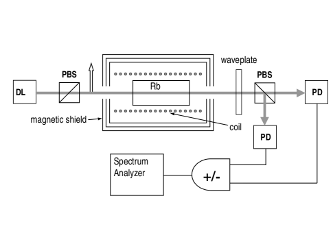
Figure 1: Experimental setup. DL: diode laser; PBS: polarizing beam splitter; PD: photodiode.

The experimental setup is sketched in Fig. 1. It consisted of a diode laser, frequency stabilized (with a saturated-absorption-based control) to the ⁸⁷Rb D1 line $F_{g}=2$ to $F_{e}=1$ transition. The laser output was linearly polarized and sent through a 5 cm long Rb vapor cell (room temperature, no buffer gas). The total light power available at the cell was 3 mW (0.5 cm² beam cross section). The cell was placed inside a three-layer mu-metal magnetic shield surrounding a solenoid that allows the scanning of a longitudinal magnetic field. After the cell, the light polarization was analyzed with a balanced polarimeter consisting of a waveplate and a polarizing beam splitter cube. Two different polarization decompositions of the light were used. When a $\lambda/4$ waveplate was present between the cell and the beam splitter the light was separated into the two orthogonal circular components ($\sigma^{+}$ and $\sigma^{-}$). If, instead, a $\lambda/2$ waveplate was used, the light was decomposed into two linear and orthogonal polarizations at $\pm 45^{\circ}$ with respect to the incident field polarization. The light intensities along the two output branches of the polarimeter were detected by similar (balanced) photodiodes with 10 MHz bandwidth. The two photocurrents were added or subtracted before being sent to an electronic spectrum analyzer with 1.8 GHz bandwidth. The spectrum analyzer was used in the zero span mode thus operating as a band-pass filter. A 2.5 MHz analysis frequency (30 kHz resolution bandwidth) was used since this frequency happened to be well separated from spurious ambient noise. The noise power was recorded as a function of the magnetic field at the cell. The experiments were carried with an extended cavity diode laser (linewidth $\lesssim$ 1 MHz) whose field fluctuations are spectrally narrower if compared with free running lasers. This choice was due to practical considerations related to the improved frequency stability and tunability of extended cavity diode lasers. We have carried some preliminary tests indicating that the use of a free running laser is also possible. Since in that case the field fluctuations have a broader spectrum, one may expect that the use of a free running laser will favor the utilization of larger analysis frequencies Camparo and Coffer (1999).

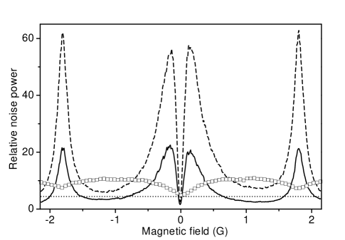
Figure 2: Observed noise power relative to shot-noise at 2.5 MHz as a function of magnetic field. Solid line: photocurrent difference noise for circular polarizations. Dashed line: photocurrent difference noise for linear polarizations. Hollow squares: Noise on the photocurrent sum for both polarization choices. Dotted line: off-resonance noise background on photocurrent sum.

The recorded signals corresponding to the noise power on the sum and difference of the two photocurrents as a function of magnetic field, for two different choices of the polarization components of the polarimeter, are presented in Fig. 2. The noise power is presented relative to the shot-noise level measured on the photocurrent difference when the laser frequency is tuned away from the atomic resonance. Also shown by the dotted line in Fig. 2 is the excess intensity-noise level (6.5 $\pm$ 0.1 dB above the shot-noise) existing on the off-resonance light. Around $B=0$, the noise on the photocurrent sum presents a reduction (to a level approaching the excess-noise level) due to the occurrence of EIT. In addition, smaller reduction of the sum noise are observed on two sidebands occurring when the magnetic field induces a Zeeman shift of the ground state Zeeman sublevels corresponding to one half of the analysis frequency (The Zeeman shift for the 5P${}_{1/2}\left(F=2\right)$ level of ⁸⁷Rb is $0.7$ MHz/Gauss). The photocurrent difference noise is dominant for small values of $B$ (corresponding to the occurrence of the EIT resonance) and at the sidebands indicating anti-correlation of the field fluctuations. A sharp ($100\%$ contrast) decrease in the photocurrent difference noise occurs for exact cancellation of the magnetic field where the noise drops below the off-resonance excess-noise level (dotted line) down to the shot-noise level (corresponding to 1 in the units used on the vertical axis of Fig. 2). As discussed below, this complete cancellation of the atomic contribution to the photocurrent difference noise is a consequence of the symmetry existing between the two polarization components when $B=0$. Rather similar shapes in the magnetic field dependence of the photocurrent difference noise are observed for circular and linear polarizations. In the latter case the noise power is increased ($4.1$ $\pm 0.7$ dB around $B=0$). The intensity dependence of the central feature of the photocurrent difference noise for circular polarizations is shown in Fig. 3. The doublet narrows and decreases as the light intensity is reduced. The narrowest observed doublet corresponds to a 70 mG separation between maxima. A similar narrowing and reduction is observed on the central dip on the photodetector sum signal noise (not shown).

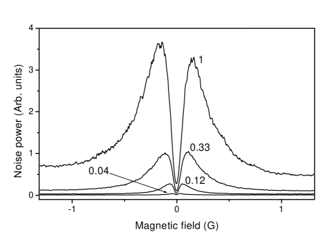
Figure 3: Central structure of the noise power signal at 2.5 MHz for circular polarizations as a function of magnetic field for various light intensities. The relative light power is indicated.

III Theory.

We present in this section a simple theoretical analysis of the interaction of an atomic system and a fluctuating light field leading to the calculation of balanced detection signals. The model is intended for an electric-dipole-allowed atomic transition between two energy levels with arbitrary angular momentum degeneracy. The transmitted field is analyzed along arbitrary polarization components. The calculation is a direct extension of previous treatments Lezama et al. (2000); Valente et al. (2003) with the inclusion of a fluctuating component on the incident field. The field is assumed to present small time dependent fluctuations around a constant nonzero mean value. This assumption allows the calculation of the atomic fluctuations through a linear response theory Jyotsna and Agarwal (1995).

We consider two degenerate levels: a ground level $g$ of total angular momentum $F_{g}$ and energy $0$ and an excited state $e$ of angular momentum $F_{e}$ and energy $\hbar\omega_{0}$. The total radiative relaxation coefficient of level $e$ is $\Gamma$. We assume that the atoms in the excited state radiatively decay into the ground state $g\$at the rate $\eta\Gamma$, where $\eta$ is a branching ratio coefficient that depends on the specific atomic transition [$0\leq\eta\leq 1$; $\eta=1$ for a closed (cycling) transition]. We consider a homogeneous ensemble of atoms at rest. However, in order to simulate the effect of a finite interaction time of the atoms with the light, we assume that the atoms escape the interaction region at a rate $\gamma$ ($\gamma\ll\Gamma$). This escape is compensated, in steady-state, by the arrival of fresh atoms in the ground state.

The incident field is $\mathbf{E}(t)=E\mathbf{e}e^{i\omega_{L}t}+E^{*}\mathbf{e}^{*}e^{-i\omega_{L}t}$ where $E$ is the complex amplitude and $\mathbf{e}$ is a unit polarization vector.

The atom field coupling in the rotating wave approximation (RWA) is:

$$W = \hbar\Omega\mathbf{e}.\mathbf{Q}_{ge}e^{i\omega_{L}t}+HC$$

$$= \hbar\left(V_{ge}e^{i\omega_{L}t}+V_{eg}e^{-i\omega_{L}t}\right)\;.$$

Here $\mathbf{Q}_{ge}=P_{g}\mathbf{Q}P_{e}$ where $P_{g}$ and $P_{e}$ are the projectors on ground and excited state manifolds respectively. The dimensionless operator $\mathbf{Q}$ is related to the atomic electric dipole operator through:

$$\mathbf{D}=\left\langle g\|\mathbf{D}\|e\right\rangle\mathbf{Q}\;,$$ (4)

where $\left\langle g\|\mathbf{D}\|e\right\rangle$ is the reduced matrix element of the dipole operator between the ground and excited state (considered real). $2\Omega=\left\langle g\|\mathbf{D}\|e\right\rangle E/\hbar$ is the reduced Rabi frequency of the field.

The total Hamiltonian in the RWA is: $H=H_{0}+W$ where $H_{0}=\hbar\omega_{0}P_{e}+(\beta_{g}P_{g}+\beta_{e}P_{e})F_{z}B$ is the atomic Hamiltonian including the Zeeman coupling with the magnetic field $B$ ($\beta_{g}$ and $\beta_{e}$ are the ground and excited sate gyromagnetic factors and $F_{z}$ is the total angular momentum projection along the magnetic field).

The evolution of the atomic density matrix $\rho$ is governed by the Bloch equation:

$$\dot{\rho} = -\frac{i}{\hbar}\left[H_{0}+W,\rho\right]-\frac{\Gamma}{2}\left\{P_{e},\rho\right\}$$

$$+\eta\Gamma\left(2F_{e}+1\right)\sum_{q=-1,0,1}Q_{ge}^{q}\rho Q_{eg}^{q}-\gamma\left(\rho-\rho_{0}\right)\;.$$

$\ Q_{ge}^{q}=Q_{eg}^{q\dagger}\ \ (q=-1,0,1)$ are the standard components of $\mathbf{Q}$ and $\gamma\rho_{0}$ represents a constant pumping rate (due to the arrival of fresh atoms) in the isotropic state $\rho_{0}=P_{g}/\left(2F_{g}+1\right)$.

After traversing an optically thin atomic medium, the transmitted field is given by Walser and Zoller (1994):

$$\mathbf{\varepsilon}\left(t\right) = \left(\mathbf{E}+i\kappa\mathbf{P}\right)e^{i\omega_{L}t}$$ (6)

$$= \left[\mathbf{\alpha}\left(t\right)+i\mathbf{\beta}\left(t\right)\right]e^{i\omega_{L}t}\;,$$ (7)

where $\kappa$ is a constant dependent on the optical thickness of the sample. We assume that both $\mathbf{\alpha}\left(t\right)$ and $\mathbf{\beta}\left(t\right)$ are stationary fluctuating (complex) quantities corresponding to the incident field and to the field radiated by the atoms respectively. We write:

$$\mathbf{\alpha}\left(t\right) = \left[\bar{\alpha}+\delta\alpha\left(t\right)\right]\mathbf{e}$$ (8)

$$\mathbf{\beta}\left(t\right) = \mathbf{\bar{\beta}}+\delta\mathbf{\beta}\left(t\right)\;,$$ (9)

with $\overline{\delta\alpha\left(t\right)}=0$ and $\overline{\delta\mathbf{\beta}\left(t\right)}=0$ (the upper bar indicating a stochastic average).

The output field component with complex polarization $\mathbf{q}$ is $\varepsilon_{q}\left(t\right)\equiv\mathbf{q}^{\ast}\cdot\mathbf{\varepsilon}\left(t\right)\equiv\bar{\varepsilon}_{q}+\delta\varepsilon_{q}\left(t\right)\equiv\left(\alpha_{q}+i\beta_{q}\right)+\left[\delta\alpha_{q}\left(t\right)+i\delta\beta_{q}\left(t\right)\right]$ and the corresponding intensity:

$$I_{q}\left(t\right) = \left|\bar{\varepsilon}_{q}\right|^{2}+\delta I_{q}\left(t\right)$$ (10)

$$\delta I_{q}\left(t\right) \simeq \left(\alpha_{q}^{\ast}-i\beta_{q}^{\ast}\right)\left[\delta\alpha_{q}\left(t\right)+i\delta\beta_{q}\left(t\right)\right]+cc\;,$$ (11)

where only linear noise contributions are retained.

Taking the Fourier transform of Eq. 11 we get:

$$\widetilde{\delta I}_{q}\left(\omega\right) \simeq \widetilde{\delta I}_{q}^{F}\left(\omega\right)+\widetilde{\delta I}_{q}^{A}\left(\omega\right)$$ (12)

$$\widetilde{\delta I}_{q}^{F}\left(\omega\right) = \left(\alpha_{q}^{*}-i\beta_{q}^{*}\right)\widetilde{\delta\alpha}_{q}\left(\omega\right)$$ (13)

$$+\left(\alpha_{q}+i\beta_{q}\right)\widetilde{\delta\alpha}_{q}^{*}\left(-\omega\right)$$

$$\widetilde{\delta I}_{q}^{A}\left(\omega\right) = i\left(\alpha_{q}^{*}-i\beta_{q}^{*}\right)\widetilde{\delta\beta}_{q}\left(\omega\right)$$ (14)

$$-i\left(\alpha_{q}+i\beta_{q}\right)\widetilde{\delta\beta}_{q}^{*}\left(-\omega\right)\;,$$

where we have identified two contributions to the light intensity fluctuations: $\widetilde{\delta I}_{q}^{F}\left(\omega\right)$ arising from the incident field fluctuations and $\widetilde{\delta I}_{q}^{A}\left(\omega\right)$ originating from the induced atomic dipole fluctuations. If the atomic dipole fluctuations can be neglected, then $\widetilde{\delta I}_{q}\left(\omega\right)\simeq\widetilde{\delta I}_{q}^{F}\left(\omega\right)$ and the only terms producing phase to amplitude noise conversion are proportional to the real part of the mean atomic dipole moment as was assumed in Eq. 1.

In general, the atomic dipole fluctuations are not negligible. We evaluate their contribution using a linear response approach. For this, we write the incident field fluctuations in the form $\delta\alpha\left(t\right)=a\left(t\right)+ib\left(t\right)$ were $a\left(t\right)$ and $b\left(t\right)$ are real fluctuating functions with zero average value. Since $\bar{\alpha}$ has been taken real, $a\left(t\right)$ [Fourier transform: $\widetilde{a}\left(\omega\right)$] represents in-phase (amplitude) fluctuations while $b\left(t\right)$ [Fourier transform: $\widetilde{b}\left(\omega\right)$] corresponds to quadrature fluctuations. In the limit of small fluctuations $b\left(t\right)$ represent phase noise. The calculation of the spectrum of transmitted field intensity fluctuations, $\widetilde{\delta I}_{q}\left(\omega\right)$, as a function of $\ \widetilde{a}\left(\omega\right)$ and $\widetilde{b}\left(\omega\right)$ is carried out in the Appendix. Further simplification is obtained under the assumption that the two quadrature noise components are totally uncorrelated [$\overline{\widetilde{a}\left(\omega\right)\widetilde{b}\left(\omega^{\prime}\right)}=\overline{\widetilde{a}\left(\omega\right)\widetilde{b}^{\ast}\left(\omega^{\prime}\right)}=0$]. The expression for the cross-correlation spectrum $S_{qq^{\prime}}\left(\omega\right)\equiv\overline{\widetilde{\delta I}_{q}\left(\omega\right)\widetilde{\delta I}_{q^{\prime}}^{\ast}\left(\omega\right)}$ is obtained in the Appendix in the form:

$$S_{qq^{\prime}}\left(\omega\right)=G_{qq^{\prime}}^{a}\left(\omega\right)\overline{\left|\widetilde{a}\left(\omega\right)\right|^{2}}+G_{qq^{\prime}}^{b}\left(\omega\right)\overline{\left|\widetilde{b}\left(\omega\right)\right|^{2}}$$ (15)

(see Eq. 39) showing that the intensity noise spectrum can be derived from the knowledge of the noise power spectra on the two quadratures of the incident field. It should be mentioned that in the case of diode lasers, correlations between phase and amplitude fluctuations are known to play a significant role Henry (1982); Vahala et al. (1983) and consequently Eq. 15 should only be considered as approximative. However, in the following section the amplitude fluctuations will be neglected ($\widetilde{a}\left(\omega\right)=0$) in which case Eq. 15 can be consistently used.

In a balanced detection experiment, two photodiodes record the light intensities corresponding to two orthogonal polarizations $\mathbf{q}$ and $\mathbf{q}^{\prime}$ respectively. The fluctuation power spectra of the sum [$Z_{+}\left(\omega\right)$] and difference [$Z_{-}\left(\omega\right)$] of the two photocurrents are given by:

$$Z_{\pm}\left(\omega\right)=S_{qq}\left(\omega\right)+S_{q^{\prime}q^{\prime}}\left(\omega\right)\pm S_{qq^{\prime}}\left(\omega\right)\pm S_{q^{\prime}q}\left(\omega\right)$$ (16)

IV Numerical results.

We present in this section the transmitted field noise spectra calculated from the model above. Having the comparison with experimental results in mind, we restrict ourselves to a limited choice of the parameters within the large freedom allowed by the model. We consider a model atomic transition $F_{g}=1\rightarrow F_{e}=0$. The transition is considered closed in the sense that the radiative decay from the excited state returns the atom to the ground level ($\eta=1$ in the model). However, the transition actually behaves as an open transition due to the existence of a trapping state in the ground level Renzoni et al. (1999). Numerical simulations with more realistic choices of the atomic level angular momenta and branching ratio are straightforward and give results qualitatively similar to those presented here.

The field incident on the atomic sample is taken linearly polarized and we consider the decomposition of the transmitted light either into two orthogonal circular polarization components or two orthogonal linear polarization components.

A strong simplification is introduced based on the fact that phase noise is known to be dominant in diode lasers Zhang et al. (1995). We consider that all the incident field noise is in the quadrature component $b\left(t\right)$ [we take $a\left(t\right)=0$]. Such assumption leads to a qualitative agreement with the experimental observation. If amplitude noise is introduced in the calculation, it generally results in a dominant noise background since in this case there are intensity fluctuations at the detectors even in the absence of the atomic medium.

We calculate noise power at a fixed analysis frequency $\omega$ as a function of the longitudinal magnetic field $B$. This calculation does not require the knowledge of the incident field spectrum. According to Eq. 15, only the value of $\overline{\left|\widetilde{b}\left(\omega\right)\right|^{2}}$ at the analysis frequency (a scale factor) is needed. In all the calculations presented below we have used $\omega=0.3\Gamma$ ($\sim$ 2 MHz in the case of the Rb D lines). The evaluations of $\beta_{q}$, and $\widetilde{\delta\beta}_{q}\left(\omega\right)$ require the knowledge of the proportionality constant $K$ (see Eqs. 29, 34). We have taken $K=1$ which (together with $\gamma=10^{-3}\Gamma$) results in $\sim$20% weak field linear absorption (a rather realistic figure in view of the experiments).

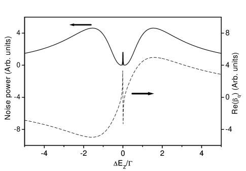
Figure 4: Solid line: noise power at $\omega=0.3\Gamma$ of a circular polarization component of the transmitted light field after interaction with an $F_{g}=1\rightarrow F_{e}=0$ atomic transition. Dashed line: real part of the mean atomic dipole along the considered circular polarization. Parameters: $\delta=0$, $\Omega=0.4\Gamma$, $\gamma=10^{-3}\Gamma$, $K=1$.

The calculated value for the noise power $S_{qq}\left(\omega\right)$ for one circular polarization component is presented as a function of the longitudinal magnetic field in Fig. 4 (in terms of the corresponding Zeeman energy shift: $\Delta E_{Z}=g\mu_{B}B$). In this plot, the atom field detuning $\delta=\omega_{0}-\omega_{L}$ is taken as zero. The noise spectrum is mainly composed of two broad peaks symmetric around $B=0$ with width and separation of the order of $\Gamma$ and a narrow structure (a doublet) of characteristic width much smaller than $\Gamma$. The broad structure arises from a linear magneto-optical effect: the circular birefringence resulting in the dephasing of one circular field component with respect to the incident field. As discussed above, such dephasing results in phase to amplitude noise conversion. The central structure is a result of the NMOE occurring near zero magnetic field owing to ground state coherence. For comparison, we show in the same figure the real part of the mean induced atomic dipole along the circular polarization considered. Notice the steep variation around $B=0$. The zero-crossing of the real part of the mean induced atomic dipole results in the doublet structure and the exact cancellation of the noise at $B=0$. At low intensities the width of the narrow structure is determined by $\gamma$.

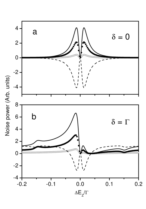
Figure 5: Nonlinear magneto-optical effect on noise power. Solid line: noise power $S_{qq}\left(\omega\right)$ for a single circular component. Solid circles: contribution to $S_{qq}\left(\omega\right)$ of $\widetilde{\delta I}_{q}^{A}\left(\omega\right)$. Hollow circles: contribution to $S_{qq}\left(\omega\right)$ of $\widetilde{\delta I}_{q}^{F}\left(\omega\right)$. Dashed line: cross-correlation noise power $S_{qq^{\prime}}\left(\omega\right)$ for the two orthogonal circular components. a) $\delta=0$, b) $\delta=\Gamma$. Other parameters: $\omega=0.3\Gamma$, $\Omega=\Gamma$, $\gamma=10^{-3}\Gamma$, $K=1$.

A closer look into the central NMO structure is presented in Fig. 5. The plot of the noise power $S_{qq}\left(\omega\right)$ (solid line) is shown together with the contributions to the noise power of the two terms $\widetilde{\delta I}_{q}^{F}\left(\omega\right)$ and $\widetilde{\delta I}_{q}^{A}\left(\omega\right)$ identified in Eq. 12 (circles). Also shown in Fig. 5a is the cross-correlation spectrum $S_{qq^{\prime}}\left(\omega\right)$ for the two different (orthogonal) circular polarizations. In the present case of $\delta=0$, we have $S_{qq^{\prime}}\left(\omega\right)=-S_{qq}\left(\omega\right)$ and consequently $Z_{+}\left(\omega\right)=0$ and $Z_{-}\left(\omega\right)=4S_{qq}\left(\omega\right)$.

In figure 5b a nonzero laser-atom detuning was used. We have taken $\delta=\Gamma$ as a representative example. Notice the asymmetry in the plot of $S_{qq}\left(\omega\right)$. Such asymmetry is expected since, for zero detuning, a given circular polarization of the field will get closer or farther to resonance depending on the magnetic field sign. Nevertheless, the cross-correlation spectrum $S_{qq^{\prime}}\left(\omega\right)$ remains symmetric with respect to $B=0$. Another significant feature in Fig. 5b is the presence in both $S_{qq}\left(\omega\right)$ and $S_{qq^{\prime}}\left(\omega\right)$ of sidebands occurring for values of the magnetic field for which the Zeeman shift $\Delta E_{Z}$ satisfies $2\Delta E_{Z}=\hbar\omega$ ($\Delta E_{Z}/\Gamma=0.15$ for the parameters of Fig. 5) Budker et al. (2002b). One can check from Fig. 5b that these sidebands are entirely due to the $\widetilde{\delta I}_{q}^{A}\left(\omega\right)$ contribution.

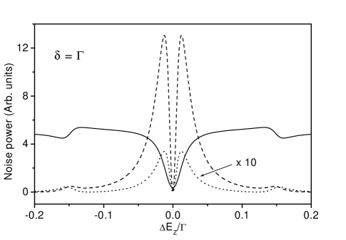
Figure 6: Calculated balanced detector noise signals. Dashed: photocurrent difference noise for circular polarizations. Dotted: photocurrent difference noise for linear polarizations. Solid: photocurrent sum noise for both polarization choices. $\delta=\Gamma$, $\omega=0.3\Gamma$, $\Omega=\Gamma$, $\gamma=10^{-3}\Gamma$, $K=1$.

The plots of the calculated intensity sum and difference noise signals, $Z_{+}\left(\omega\right)$ and $Z_{-}\left(\omega\right)$ respectively, for the choice of parameters of Fig. 5b in a balanced polarimeter in which the field is decomposed into orthogonal circular polarization components are shown in Fig. 6.  $Z_{+}\left(\omega\right)$, the total transmitted intensity noise, presents a broad background level owing to linear phase to amplitude noise conversion produced by the nonzero real part of the mean atomic polarization. Along with this broad linear contribution, $Z_{+}\left(\omega\right)$ presents narrow NMO structures: the central dip and the sidebands. The central dip is easily understood by noticing that at $B=0$ the condition is met for coherence population trapping (CPT) among Zeeman sublevels which result in electromagnetically induced transparency (EIT). The sidebands are due to resonances in the atomic fluctuations when the analysis frequency corresponds to twice the atomic Larmor frequency. The photocurrent difference noise $Z_{-}\left(\omega\right)$ is dominated by the central doublet which is related to the nonlinear circular birefringence occurring around $B=0$. For a nonzero magnetic field, the two circular polarizations of the induced atomic dipole are dephased in opposite directions resulting in anti-correlated light fluctuations. As a result of the symmetry existing at $B=0$ for the two polarization components we have $S_{qq}\left(\omega\right)=S_{q^{\prime}q^{\prime}}\left(\omega\right)=S_{qq^{\prime}}\left(\omega\right)=S_{q^{\prime}q}\left(\omega\right)$ and consequently $Z_{-}\left(\omega\right)$ cancels at this point. The dependence of $\ Z_{-}\left(\omega\right)$ (for orthogonal circular polarizations) on the light intensity is presented in Fig. 7.

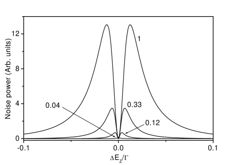
Figure 7: Intensity dependence of the balanced detector photocurrent difference noise signal $Z_{-}\left(\omega\right)$ for circular polarizations. The corresponding values of $\left(\Omega/\Gamma\right)^{2}$ are indicated ($\delta=\Gamma$, $\omega=0.3\Gamma$, $\gamma=10^{-3}\Gamma$, $K=1$).

Let us discuss now the case of a balanced detector polarimeter in which the two orthogonal output polarizations $\mathbf{q}$ and $\mathbf{q}^{\prime}$ are linear. In such a case, if the laser-atom detuning $\delta$ is zero the output light fluctuations are zero on both polarizations. This is a somehow surprising result since the nonlinear Faraday effect results in the rotation of the mean transmitted field polarization. However, in this case the real part of the induced atomic polarization along the two components $\mathbf{q}$ and $\mathbf{q}^{\prime}$ is zero (i.e. the interaction is purely absorptive) and thus no phase to noise conversion occurs. The situation is different for nonzero $\delta$. The curves corresponding to $S_{qq}\left(\omega\right)$ and $S_{qq^{\prime}}\left(\omega\right)$ for $\delta=\Gamma$ are presented in Fig. 8. The corresponding trace for $Z_{-}\left(\omega\right)$ is shown in Fig. 6   ($Z_{+}\left(\omega\right)$ is the same than for circular polarizations). Notice the significant reduction of $Z_{-}\left(\omega\right)$ in comparison with the result obtained for circular polarizations. Such behavior is in contrast with the experimental observation where an increase in the photocurrent difference noise is observed for linear polarization. We will discuss this discrepancy in the next section.

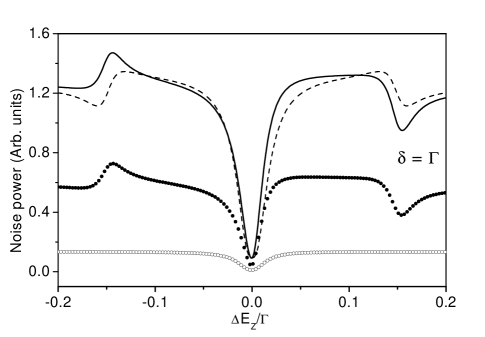
Figure 8: Nonlinear magneto-optical effect on noise power. Solid line: noise power $S_{qq}\left(\omega\right)$ for a single linear polarization component. Solid circles: contribution to $S_{qq}\left(\omega\right)$ of $\widetilde{\delta I}_{q}^{A}\left(\omega\right)$. Hollow circles: contribution to $S_{qq}\left(\omega\right)$ of $\widetilde{\delta I}_{q}^{F}\left(\omega\right)$. Dashed line: cross-correlation noise power $S_{qq^{\prime}}\left(\omega\right)$ for the two orthogonal linear polarization components. $\delta=\Gamma$, $\omega=0.3\Gamma$, $\Omega=\Gamma$, $\gamma=10^{-3}\Gamma$, $K=1$.

V Discussion.

The traces presented in Fig. 2 provide a clear demonstration of the use of noise analysis for the observation of NMOE. The observed features (much narrower than the optical transition linewidth $\Gamma$) are the consequence of ground state coherence. As in the usual ground state Hanle effect and other NMOE, a coherence resonance is observed around $B=0$. Additional resonances of comparable width are also observed when the magnetic field induces a precession of the ground state alignment at one half of the analysis frequency. Such resonances may be understood as Raman resonances between the laser carrier frequency and the “sidebands” produced by the light “modulation” produced by the spectral component of the noise at the analysis frequency.

The similarity between the experimental observations and the calculations (Fig. 6) is apparent. It suggests that the essential ingredients of the NMO noise effects are contained in the simple model considered.

However, several important differences between the model assumptions and the actual experimental conditions must be mentioned. The first concerns the fact that the numerical calculations were made for a homogeneous sample of atoms while the experiment is carried out on a vapor cell where different atoms experience different detunings $\delta$, owing to the Doppler effect. Numerical integration over $\delta$ is straightforward. The resulting curves for the balanced detection signals preserve the shape of the central feature but do not present the relatively large weight of the sidebands observed in the experiments. Our second comment concerns the naive description of the laser noise. As already mentioned, the laser amplitude noise was completely neglected. In the context of the model this appears to be a reasonable assumption since even modest amounts of amplitude noise (compared to quadrature noise) result in a magnetic-field-independent signal background. Moreover, diode lasers are known to possess phase noise in excess of amplitude noise over a wide bandwidth. Nevertheless, this simplification is quite restrictive since in addition to ignoring the small but non-negligible amplitude noise present in diode lasers, it prevents the description within the model of the effect of shot-noise. Another important simplification in the theory above is the linearized treatment of the field noise as due to small fluctuations around a constant mean value. Such a treatment is not appropriate when the field phase experiences random fluctuations resulting in phase diffusion. In the present experimental conditions, the phase diffusion time of our laser is of the order of a microsecond (inverse of the laser linewidth), which is short compared to the temporal evolution of coherence resonances. This suggests that the treatment of the laser light as a phase-diffusing field should be more appropriate. We have carried out a calculation using a phase-diffusing field model that will be presented elsewhere.

A striking difference between the experimental and the theoretical curves concerns the relative amplitude of the photocurrent difference noise for circular and linear polarizations. While the experimental result is that the noise is enhanced for linear polarizations by a factor of approximately two, the calculation shows a strong noise reduction (see Fig. 6). We believe this to be a consequence of the inadequacy of the linear model. As a matter of fact, preliminary results obtained with a phase diffusing field model show, in this respect, a good agreement with the experimental observation.

Another important difference between theoretical and experimental traces is the weight of the sidebands. The large contribution to the noise occurring at the sidebands appears to be out of reach for our present theoretical approach. This suggests that new key ingredients such as correlated amplitude and phase fluctuations, propagation effects in optically thick media or the influence of resonance fluorescence scattered into the detected light modes Ries et al. (2003), must be considered for a more accurate theoretical description.

VI Conclusions.

We have shown that noise analysis provides a useful handle for the study of NMOE. Our experiments reveal NMO features observed with large contrast and resolution without the use of any light frequency modulation other than noise modulation intrinsically present in any light source. The technique presented here can be easily applied to other elements and transitions. Since laser sources frequently present a broad noise spectrum, the noise detection of NMOE can be used over a large dynamic range of analysis frequencies, allowing the observation of coherent features for relatively large values of the magnetic field (several Gauss). On the other hand, application of the noise detection technique to paraffin coated or buffer gas cells should allow the observation of coherence resonances in the $\mu$G range. Noise detected NMO resonances may therefore be of interest for high precision magnetometry.

We have presented a simple and rather general theoretical treatment for the calculation of the spectral properties of the noise signals available in a balanced detection experiment. Good qualitative correspondence between the predictions of the model and the observations was obtained. However, some features, mainly the weight and shapes of the sideband resonances and the observed dependence of the noise signals on the orthogonal polarization decomposition, strongly suggest that a more precise treatment of the optical field fluctuations (including quantum fluctuations) and the atomic medium may be necessary. Additional work along this line is currently underway.

Appendix A

We present in this appendix the steps leading to the calculation of the noise spectral signals observed in a balanced detection polarimeter. We initially transform the Bloch equation Eq. III using a Liouville space representation. Later on, the linear response of the atomic dipole to the incident fluctuating field is derived and the spectral signals calculated.

A.1 Liouville space representation.

We consider a complex vectorial space $\mathbb{L}$ of dimension given by the number of elements in $\rho$. To each density matrix $\rho$ in Hilbert space we associate a (column) vector $y$ in $\mathbb{L}$ in such way that each matrix element in $\rho$ corresponds to an element of $y$.

$$\rho\longleftrightarrow y$$ (17)

For an operator $O$ acting upon $\rho$ we have:

$$O\rho \longleftrightarrow \mathcal{L}\left(O\right)y$$ (18)

$$\rho O \longleftrightarrow \mathcal{R}\left(O\right)y\;,$$

where $\mathcal{L}\left(O\right)$ and $\mathcal{R}\left(O\right)$ are linear operators in $\mathbb{L}$.

Let $u$ be the vector in $\mathbb{L}$ with all elements corresponding to populations equal to one and all elements corresponding to coherences equal to zero. We note for further use that $trace\left(O\rho\right)=u^{\dagger}\mathcal{L}\left(O\right)y$.

After some algebra, one can show that the Bloch equation Eq. III can be written in the form Walser and Zoller (1994):

$$\dot{y}=\exp\left(-i\mathcal{N}\omega_{L}t\right)\mathcal{A}\exp\left(i\mathcal{N}\omega_{L}t\right)y+\gamma y_{0}$$ (19)

with:

$$\mathcal{N} = \mathcal{L}\left(P_{e}\right)\mathcal{-R}\left(P_{e}\right)$$ (20)

$$\mathcal{A} \equiv -\frac{i}{\hbar}\left[\mathcal{L}\left(H_{0}+V\right)-\mathcal{R}\left(H_{0}+V\right)\right]$$ (21)

$$-\frac{\Gamma}{2}\left[\mathcal{L}\left(P_{e}\right)+\mathcal{R}\left(P_{e}\right)\right]-\gamma\mathbb{I}$$

$$+\eta\Gamma\left(2F_{e}+1\right)\sum_{q=-1,0,1}\mathcal{L}\left(Q_{ge}^{q}\right)\mathcal{R}\left(Q_{eg}^{q}\right)$$

$$\rho_{0} \longleftrightarrow y_{0}$$ (22)

where $\mathbb{I}$ is the identity operator in $\mathbb{L}$ and $V=V_{ge}+V_{eg}$ (see Eq. III).

It is convenient to consider the Liouville space vector $x=\exp\left(i\mathcal{N}\omega_{L}t\right)y$ entirely composed by slowly varying coefficients. Substitution in Eq. 19 gives:

$$\dot{x}=\left(i\mathcal{N}\omega_{L}+\mathcal{A}\right)x+\gamma y_{0}\;.$$ (23)

After solving 23, the slowly varying envelope of the atomic polarization can be obtained through:

$$\mathbf{P}\left(t\right)=u^{\dagger}\mathcal{L}\left(\mathbf{D}_{eg}\right)x\left(t\right)\;.$$ (24)

A.2 Fluctuating atomic response.

We seek a solution of Eq. 23 in the form $x\left(t\right)=\bar{x}+\delta x\left(t\right)$. Linearizing Eq. 23 we have the following system:

$$0 = \mathcal{B}\left(\bar{\alpha}\right)\bar{x}+\gamma y_{0}$$ (25)

$$\delta\dot{x}\left(t\right) = \mathcal{B}\left(\bar{\alpha}\right)\delta x\left(t\right)$$ (26)

$$-\left[\mathcal{D}^{-}\delta\alpha\left(t\right)+\mathcal{D}^{+}\delta\alpha^{\ast}\left(t\right)\right]\bar{x}$$

$$\mathcal{D}^{-} \equiv \frac{i}{\hbar}\left[\mathcal{L}\left(\mathbf{e}.\mathbf{D}_{ge}\right)-\mathcal{R}\left(\mathbf{e}.\mathbf{D}_{ge}\right)\right]$$ (27)

$$\mathcal{D}^{+} \equiv \frac{i}{\hbar}\left[\mathcal{L}\left(\mathbf{e}^{\ast}.\mathbf{D}_{eg}\right)-\mathcal{R}\left(\mathbf{e}^{\ast}.\mathbf{D}_{eg}\right)\right]\;,$$ (28)

where $\mathcal{B}\equiv i\mathcal{N}\omega_{L}+\mathcal{A}$ and we have taken advantage of the fact that $\mathcal{A}$ is linear on the complex field amplitudes $\alpha\left(t\right)$ and $\alpha^{\ast}\left(t\right)$ (see Eq. 21). Eq. 25 gives the mean value $\bar{x}$ from which the average atomic dipole components $\beta_{q}$ can be obtained (using Eq. 24) as:

$$\beta_{q}=Ku^{\dagger}\mathcal{L}\left(\mathbf{q}^{\ast}\cdot\mathbf{D}_{eg}\right)\bar{x}\;,$$ (29)

where $K$ is a proportionality constant.

Taking the Fourier transform of Eq. 26:

$$\widetilde{\delta x}\left(\omega\right)=\left[i\omega\mathbb{I}+\mathcal{B}\left(\bar{\alpha}\right)\right]^{-1}\left[\mathcal{D}^{-}\widetilde{\delta\alpha}\left(\omega\right)+\mathcal{D}^{+}\widetilde{\delta\alpha}^{\ast}\left(-\omega\right)\right]\bar{x}\;,$$ (30)

we notice that $\widetilde{\delta x}\left(\omega\right)$ presents a resonant behavior for $\omega$ approaching the eigenfrequencies of the evolution operator $\mathcal{B}\left(\bar{\alpha}\right)$.

We proceed by writing $\delta\alpha\left(t\right)=a\left(t\right)+ib\left(t\right)$, where $a\left(t\right)$ and $b\left(t\right)$ are real fluctuating functions with zero mean value. Using the corresponding Fourier transforms, $\widetilde{a}\left(\omega\right)$ and $\widetilde{b}\left(\omega\right)$, in Eq. 30 we have:

$$\widetilde{\delta x}\left(\omega\right) = \left[i\omega\mathbb{I}+\mathcal{B}\left(\bar{\alpha}\right)\right]^{-1}\left[\left(\mathcal{D}^{-}+\mathcal{D}^{+}\right)\widetilde{a}\left(\omega\right)\right.$$ (31)

$$\left.+i\left(\mathcal{D}^{-}-\mathcal{D}^{+}\right)\widetilde{b}\left(\omega\right)\right]\bar{x}\;,$$

and from Eq. 24 we get:

$$\widetilde{\delta\beta}_{q}\left(\omega\right)=f_{a}\left(\omega\right)\widetilde{a}\left(\omega\right)+f_{b}\left(\omega\right)\widetilde{b}\left(\omega\right)\;,$$ (32)

with

$$f_{a}\left(\omega\right) = Ku^{\dagger}\mathcal{L}\left(\mathbf{q}^{\ast}\cdot\mathbf{D}_{eg}\right)\left[i\omega\mathbb{I}+\mathcal{B}\left(\bar{\alpha}\right)\right]^{-1}$$ (33)

$$\times\left(\mathcal{D}^{-}+\mathcal{D}^{+}\right)\bar{x}$$

$$f_{b}\left(\omega\right) = Ku^{\dagger}\mathcal{L}\left(\mathbf{q}^{\ast}\cdot\mathbf{D}_{eg}\right)\left[i\omega\mathbb{I}+\mathcal{B}\left(\bar{\alpha}\right)\right]^{-1}$$ (34)

$$\times i\left(\mathcal{D}^{-}-\mathcal{D}^{+}\right)\bar{x}\;.$$

Substituting Eq. 32 into Eqs. 12-14 we write:

$$\widetilde{\delta I}_{q}\left(\omega\right)=g_{q}^{a}\left(\omega\right)\widetilde{a}\left(\omega\right)+g_{q}^{b}\left(\omega\right)\widetilde{b}\left(\omega\right)\;,$$ (35)

with

$$g_{q}^{a}\left(\omega\right) \equiv \left(\alpha_{q}^{\ast}-i\beta_{q}^{\ast}\right)\left[\left(\mathbf{q}^{\ast}\cdot\mathbf{e}\right)+if_{a}\left(\omega\right)\right]$$ (36)

$$+\left(\alpha_{q}+i\beta_{q}\right)\left[\left(\mathbf{q}\cdot\mathbf{e}^{\ast}\right)-if_{a}^{\ast}\left(-\omega\right)\right]$$

$$g_{q}^{b}\left(\omega\right) \equiv i\left(\alpha_{q}^{\ast}-i\beta_{q}^{\ast}\right)\left[\left(\mathbf{q}^{\ast}\cdot\mathbf{e}\right)+f_{b}\left(\omega\right)\right]$$ (37)

$$-\left(\alpha_{q}+i\beta_{q}\right)\left[\left(\mathbf{q}\cdot\mathbf{e}^{\ast}\right)+f_{b}^{\ast}\left(-\omega\right)\right]\ .$$

A.3 Spectrum.

We are interested in the spectral components:

$$S_{qq^{\prime}}\left(\omega\right)=\overline{\widetilde{\delta I}_{q}\left(\omega\right)\widetilde{\delta I}_{q^{\prime}}^{*}\left(\omega\right)}\;.$$ (38)

Further simplification can be obtained under the additional assumption that the two quadrature components of the noise are uncorrelated [$\overline{\widetilde{a}\left(\omega\right)\widetilde{b}\left(\omega^{\prime}\right)}=\overline{\widetilde{a}\left(\omega\right)\widetilde{b}^{*}\left(\omega^{\prime}\right)}=0$]; using Eq. 35 we get:

$$S_{qq^{\prime}}\left(\omega\right) = g_{q}^{a}\left(\omega\right)g_{q^{\prime}}^{a*}\left(\omega\right)\overline{\left|\widetilde{a}\left(\omega\right)\right|^{2}}$$ (39)

$$+g_{q}^{b}\left(\omega\right)g_{q^{\prime}}^{b*}\left(\omega\right)\overline{\left|\widetilde{b}\left(\omega\right)\right|^{2}}\;.$$

References

- Georges and Lambropoulos (1979) A. T. Georges and P. Lambropoulos, Phys. Rev. A 18, 991 (1979).
- Agarwal (1978) G. Agarwal, Phys. Rev. A 18, 1490 (1978).
- Georges (1980) A. T. Georges, Phys. Rev. A 21, 2034 (1980).
- Dalton and Knight (1982a) B. J. Dalton and P. L. Knight, Opt. Commun. 42, 411 (1982a).
- Dalton and Knight (1982b) B. J. Dalton and P. L. Knight, J. Phys. B: At. Mol. Phys. 15, 3997 (1982b).
- Elliott et al. (1985) D. S. Elliott, M. W. Hamilton, K. Arnett, and S. J. Smith, Phys. Rev. A 32, 887 (1985).
- Anderson et al. (1990) M. H. Anderson, R. D. Jones, J. Cooper, S. J. Smith, D. S. Elliott, H. Ritsch, and P. Zoller, Phys. Rev. A 42, 6690 (1990).
- Ritsch et al. (1990) H. Ritsch, P. Zoller, and J. Cooper, Phys. Rev. A 41, 2653 (1990).
- Vemuri et al. (1991) G. Vemuri, M. H. Anderson, J. Cooper, and S. J. Smith, Phys. Rev. A 44, 7635 (1991).
- Camparo and Lambropoulos (1991) J. C. Camparo and P. Lambropoulos, Opt. Commun. 85, 213 (1991).
- Jyotsna and Agarwal (1995) I. V. Jyotsna and G. Agarwal, Phys. Rev. A 51, 3169 (1995).
- Kinrot et al. (1995) O. Kinrot, I. S. Averbukh, and Y. Prior, Phys. Rev. Lett. 75, 3822 (1995).
- Camparo and Lambropoulos (1993) J. C. Camparo and P. Lambropoulos, Phys. Rev. A 47, 480 (1993).
- Scully and Zubairy (1997) M. O. Scully and M. S. Zubairy, Quantum optics (Cambridge University Press, Cambridge, 1997).
- Yabusaki et al. (1991) T. Yabusaki, T. Mitsui, and U. Tanaka, Phys. Rev. Lett. 67, 2453 (1991).
- McIntyre et al. (1993) D. H. McIntyre, C. E. Fairchild, J. Cooper, and R. Walser, Optics Lett. 18, 1816 (1993).
- Walser and Zoller (1994) R. Walser and P. Zoller, Phys. Rev. A 49, 5067 (1994).
- Rosenbluh et al. (1998) M. Rosenbluh, A. Rosenhouse-Dantsker, A. D. Wilson-Gordon, M. D. Levenson, and R. Walser, Opt. Commun. 146, 158 (1998).
- Camparo and Coffer (1999) J. C. Camparo and J. G. Coffer, Phys. Rev. A 59, 728 (1999).
- Zhang et al. (1995) T. C. Zhang, J. P. Poizat, P. Grelu, J. F. Roch, P. Grangier, F. Marin, A. Bramati, V. Jost, M. D. Levenson, and E. Giacobino, Quantum. Semiclass. Opt. 7, 601 (1995).
- Budker et al. (2002a) D. Budker, W. Gawlik, D. F. Kimball, S. M. Rochester, V. V. Yashchuk, and A. Weis, Rev. Mod. Phys 74, 1153 (2002a).
- Budker et al. (1998) D. Budker, V. V. Yashchuk, and M. Zolotorev, Phys. Rev. Lett. 81, 5788 (1998).
- Budker et al. (1999) D. Budker, D. F. Kimball, S. M. Rochester, and V. V. Yashchuk, Phys. Rev. Lett. 83, 1767 (1999).
- Budker et al. (2002b) D. Budker, D. F. Kimball, V. V. Yashchuk, and M. Zolotorev, Phys. Rev. A 65, 055403 (2002b).
- Failache et al. (2003) H. Failache, P. Valente, G. Ban, V. Lorent, and A. Lezama, Phys. Rev. A 67, 043810 (2003).
- Dupont-Roc (1970) J. Dupont-Roc, Rev. Phys. Appl. 5, 853 (1970).
- Mitusi (2000) T. Mitusi, Phys. Rev. Lett. 84, 5292 (2000).
- Matsko et al. (2002) A. B. Matsko, I. Novikova, G. R. Welch, D. Budker, D. F. Kimball, and S. M. Rochester, Phys. Rev. A 66, 043815 (2002).
- Ries et al. (2003) J. Ries, B. Brezger, and A. I. Lvovsky, Phys. Rev. A 68, 025801 (2003).
- Josse et al. (2003) V. Josse, A. Dantan, L. Vernac, A. Bramati, M. Pinard, and E. Giacobino, Phys. Rev. Lett. 91, 103601 (2003).
- Akulshin et al. (1998) A. M. Akulshin, S. Barreiro, and A. Lezama, Phys. Rev. A 57, 2996 (1998).
- Phillips et al. (2001) D. F. Phillips, A. Fleischhauer, A. Mair, R. L. Walsworth, and M. D. Lukin, Phys. Rev. Lett. 86, 783 (2001).
- Lukin and Imamoglu (2001) M. D. Lukin and A. Imamoglu, Nature 413, 273 (2001).
- Garrido Alzar et al. (2003) C. L. Garrido Alzar, L. S. Cruz, J. G. Aguirre Gómez, M. França Santos, and P. Nussenzveig, Europhys. Lett. 61, 485 (2003).
- Lezama et al. (2000) A. Lezama, S. Barreiro, A. Lipsich, and A. M. Akulshin, Phys. Rev. A 61, 013801 (2000).
- Valente et al. (2003) P. Valente, H. Failache, and A. Lezama, Phys. Rev. A 67, 013806 (2003).
- Henry (1982) C. H. Henry, IEEE J. Quantum Electron. 18, 259 (1982).
- Vahala et al. (1983) K. Vahala, C. Harder, and A. Yariv, Appl. Phys. Lett. 42, 211 (1983).
- Renzoni et al. (1999) F. Renzoni, A. Lindner, and E. Arimondo, Phys. Rev. A 60, 450 (1999).