Model reconstruction of nonlinear dynamical systems driven by noise

Abstract

An efficient technique is introduced for model inference of complex nonlinear dynamical systems driven by noise. The technique does not require extensive global optimization, provides optimal compensation for noise-induced errors and is robust in a broad range of dynamical models. It is applied to clinically measured blood pressure signal for the simultaneous inference of the strength, directionality, and the noise intensities in the nonlinear interaction between the cardiac and respiratory oscillations.

Most natural and man-made systems are inherently noisy and nonlinear. This has led to the use of stochastic nonlinear dynamical models for observed phenomena across many scientific disciplines. Examples range from lasers laser and molecular motors motors , to epidemiology epidemiology , to coupled matter–radiation systems in astrophysics astrophysics . In this approach a complex system is characterized by projecting it onto a specific dynamical model with parameters obtained from the measured time-series data. In a great number of important problems the model is not usually known exactly from “first principles” and one is faced with a rather broad range of possible parametric models to consider. Furthermore, important “hidden” features of a model such as coupling coefficients between the dynamical degrees of freedom can be very difficult to extract due to the intricate interplay between noise and nonlinearity. These obstacles render the inference of stochastic nonlinear dynamical models from experimental time series a formidable task, with no efficient general methods currently available for its solution.

Deterministic inference techniques Kantz:97 consistently fail to yield accurate parameter estimates in the presence of noise. The problem becomes even more complicated when both measurement noise as well as intrinsic dynamical noise are present Meyer:01 . Various numerical schemes have been proposed recently to deal with different aspects of this inverse problem McSharry:99 ; Heald:00 ; Meyer:00 ; Friedrich:00 ; Meyer:01 ; Rossi:02 ; Friedrich:03 . A standard approach is based on optimization of a certain cost function (a likelihood function) at the values of the model parameters that best reconstruct the measurements. It can be further generalized using a Bayesian formulation of the problem Meyer:00 ; Meyer:01 . Existing techniques usually employ numerical Monte Carlo techniques for complex optimization Rossi:02 or multidimensional integration Meyer:00 tasks. Inference results from noisy observations are shown to be very sensitive to the specific choice of the likelihood function McSharry:99 . Similarly, the correct choice of this function is one of the central questions in the inference of continuous-time noise-driven dynamical models considered here.

In this Letter, we present an efficient technique of Bayesian inference of nonlinear noise-driven dynamical models from time-series data that avoids extensive numerical optimization. It also guarantees optimum compensation of noise-induced errors by invoking the likelihood function in the form of a path integral over the random trajectories of the dynamical system. The robustness of our technique in a wide range of model parameters is verified using synthetic data from the stochastic Lorenz system. We also present the reconstruction of a nonlinear model of cardio-respiratory interaction from experimentally measured blood pressure signal.

Let the trajectory ${\bf x}(t)$ of a certain $N$-dimensional dynamical system be observed at sequential time instants $t_{0},t_{1},\ldots$ and a series ${\cal Y}=\{(t_{k},{\bf y}_{k});\,k=0:K\}$ thus be obtained. These measurements can be related to the (unknown) system trajectory through some conditional probability distribution function (PDF) $p_{\rm o}[{\cal Y}|{\bf x}(t)]$ giving the probability of observing a time series ${\cal Y}$ for a specific system trajectory ${\bf x}(t)$. If we assume that ${\bf y}_{k}$ has the same dimension as ${\bf x}(t_{k})$ and the measurement errors ${\bf y}_{k}-{\bf x}(t_{k})$ are uncorrelated Gaussian random variables with mean zero and variance $\epsilon^{2}$, then we obtain $p_{\rm o}\left({\cal Y}|{\cal X}\right)=\prod_{l=0}^{K}\,{\cal N}\,[{\bf y}_{l}-{\bf x}(t_{l}),\epsilon_{l}]$, where ${\cal X}=\{{\bf x}(t_{k})\}$.

Assume now that the underlying dynamical system is in fact nonlinear and stochastic, evolving according to

$$\dot{\bf x}(t)={\bf f}({\bf x})+{\bm{\xi}}(t),$$ (1)

where ${\bm{\xi}}(t)$ is an additive vector noise process. We parameterize this system in the following way. The nonlinear vector field ${\bf f}({\bf x})$ is written in the form

$${\bf f}({\bf x})={\hat{\bf U}}({\bf x})\,{\bf c}\equiv{\bf f}({\bf x};{\bf c}),$$ (2)

where ${\hat{\bf U}}({\bf x})$ is an $N\times M$ matrix of suitably chosen basis functions $\{U_{nm}({\bf x});\,n=1:N,\,m=1:M\}$, and ${\bf c}$ is an $M$-dimensional coefficient vector. An important feature of (2) for our subsequent development is that, while possibly highly nonlinear in ${\bf x}$, ${\bf f}({\bf x};{\bf c})$ is strictly linear in ${\bf c}$. Dynamical noise ${\bm{\xi}}(t)$ may also be parameterized. For instance, if ${\bf\xi}(t)$ is stationary white and Gaussian

$$\langle{\bm{\xi}}(t)\rangle=0,\quad\langle{\bm{\xi}}(t)\,{\bm{\xi}}^{T}(t^{\prime})\rangle={\hat{\bf D}}\,\delta(t-t^{\prime}),$$ (3)

then the $N\times N$ (symmetric) noise covariance matrix ${\hat{\bf D}}$ fully parameterizes the noise. The vector elements $\{c_{m}\}$ and the matrix elements $\{D_{nn^{\prime}}\}$ together constitute a set ${\cal M}=\{{\bf c},{\hat{\bf D}}\}$ of unknown parameters to be inferred from the measurements ${\cal Y}$.

In the Bayesian model inference, two distinct PDFs are ascribed to the set of unknown model parameters: the prior $p_{\textrm{pr}}({\cal M})$ and the posterior $p_{\textrm{post}}({\cal M}|{\cal Y})$, respectively representing our state of knowledge about ${\cal M}$ before and after processing a block of data ${\cal Y}$. The two PDFs are related to each other via Bayes’ theorem:

$$p_{\textrm{post}}({\cal M}|{\cal Y})=\frac{{\ell}({\cal Y}|{\cal M})\,p_{\textrm{pr}}({\cal M})}{\int\ell({\cal Y}|{\cal M})\,p_{\textrm{pr}}({\cal M})\,{\rm d}{\cal M}}.$$ (4)

Here $\ell({\cal Y}|{\cal M})$, usually termed the likelihood, is the conditional PDF of the measurements ${\cal Y}$ for a given choice ${\cal M}$ of the dynamical model. In practice, (4) can be applied iteratively using a sequence of data blocks ${\cal Y},{\cal Y}^{\prime}$, etc. The posterior computed from block ${\cal Y}$ serves as the prior for the next block ${\cal Y}^{\prime}$, etc. For a sufficiently large number of observations, $p_{\textrm{post}}({\cal M}|{\cal Y},{\cal Y}^{\prime},\ldots)$ is sharply peaked at a certain most probable model $\cal M={\cal M}^{\ast}$.

We specify a prior distribution $p_{\textrm{pr}}({\cal M})$ that is Gaussian with respect to elements of ${\bf c}$ and uniform with respect to elements of ${\bf\hat{D}}$. Thus, $p_{\textrm{pr}}({\cal M})={\cal N}({\bf c}-{\bf c}_{\textrm{pr}},{\hat{\bm{\Sigma}}}_{\textrm{pr}})$, where the mean ${\bf c}_{\textrm{pr}}$ and the covariance ${\hat{\bm{\Sigma}}}_{\textrm{pr}}$ respectively encapsulate our knowledge and associated uncertainty about the coefficient vector ${\bf c}$. We now write the expression for the likelihood in the form of a path integral over the random trajectories of the system:

$$\ell({\cal Y}|{\cal M})=\int_{{\bf x}(t_{\rm i})}^{{\bf x}(t_{\rm f})}p_{\rm o}({\cal Y}|{\cal X})\,{\cal F}_{\cal M}[{\bf x}(t)]\,{\cal D}{\bf x}(t),$$ (5)

where we choose $t_{\rm i}\ll t_{0}<t_{K}\leqslant t_{\rm f}$ so that $\ell$ does not depend on the particular initial and final states ${\bf x}(t_{\rm i})$, ${\bf x}(t_{\rm f})$. The form of the probability functional ${\cal F}_{\cal M}$ over the system trajectory ${\bf x}(t)$ is determined by the properties of the dynamical noise ${\bm{\xi}}(t)$ Graham:77 ; Dykman:90 .

In this Letter, we are focusing on the case of Gaussian white noise, as indicated in (1), (3). We consider a uniform sampling scheme $t_{k}=t_{0}+hk$, $h\equiv(t_{K}-t_{0})/K$ and assume that for each trajectory component $x_{n}(t)$ the measurement error $\epsilon$ is negligible compared with the fluctuations induced by the dynamical noise; that is, $\epsilon^{2}\ll h({\bf\hat{D}}^{2})_{n\,n}$. Consequently, we use $p_{\rm o}({\cal Y}|{\cal X})\rightarrow\prod_{k=0}^{K}\delta[{\bf y}_{k}-{\bf x}(t_{k})]$ in (5). Using results from Graham:77 for ${\cal F}_{\cal M}[{\bf x}(t)]$, the logarithm of the likelihood (5) takes the following form for sufficiently large $K$ (small time step $h$):

$$-\frac{2}{K}\log\ell({\cal Y}|{\cal M})=\ln\det{\hat{\bf D}}+\frac{h}{K}\sum_{k=0}^{K-1}\left[\,\,\mathop{\rm tr}{\hat{\bf\Phi}}({\bf y}_{k};{\bf c})\right.$$ (6)

$$\left.+(\dot{\bf y}_{k}-{\bf f}({\bf y}_{k};{\bf c}))^{T}\,{\hat{\bf D}}^{-1}\,(\dot{\bf y}_{k}-{\bf f}({\bf y}_{k};{\bf c}))\right]+N\ln(2\pi h),$$

here we introduce the “velocity” $\dot{\bf y}_{k}$ and matrix ${\bf\hat{\Phi}}({\bf x})$

$$\dot{\bf y}_{k}\equiv h^{-1}({\bf y}_{k+1}-{\bf y}_{k}),\quad({\hat{\bf\Phi}}({\bf x};{\bf c}))_{n\,n^{\prime}}\equiv\partial f_{n}({\bf x};{\bf c})/\partial x_{n^{\prime}}.$$

With the use of (2), substitution of the prior $p_{\textrm{pr}}({\cal M})$ and the likelihood $\ell({\cal Y}|{\cal M})$ into (4) yields the posterior $p_{\textrm{post}}({\cal M}|{\cal Y})={\rm const}\times\exp[-S({\cal M}|{\cal Y})]$, where

$$S({\cal M}|{\cal Y})\equiv S_{\textsf{y}}({\bf c},{\bf\hat{D}})=\frac{1}{2}\rho_{\textsf{y}}({\bf\hat{D}})-{\bf c}^{T}{\bf w}_{\textsf{y}}({\bf\hat{D}})+\frac{1}{2}{\bf c}^{T}{\bf\hat{\Xi}}_{\textsf{y}}({\bf\hat{D}}){\bf c}.$$ (7)

Here, use was made of the definitions

$$\hskip 3.25201pt\rho_{\textsf{y}}({\bf\hat{D}})=h\,\sum_{k=0}^{K-1}\dot{{\bf y}}_{k}^{T}\,{\bf\hat{D}}^{-1}\,\dot{{\bf y}}_{k}+K\,\ln(\det{\bf\hat{D}}),$$ (8)

$${\bf w}_{\textsf{y}}({\bf\hat{D}})={\bf\hat{\Sigma}}_{\textrm{pr}}^{-1}\,{\bf c}_{\textrm{pr}}+h\sum_{k=0}^{K-1}\left[{\bf\hat{U}}_{k}^{T}\,{\bf\hat{D}}^{-1}\,\dot{{\bf y}}_{k}-\frac{1}{2}{\bf v}({\bf y}_{k})\right],$$

$${\bf\hat{\Xi}}_{\textsf{y}}({\bf\hat{D}})={\bf\hat{\Sigma}}^{-1}_{\textrm{pr}}+h\,\sum_{k=0}^{K-1}{\bf\hat{U}}_{k}^{T}\,{\bf\hat{D}}^{-1}\,{\bf\hat{U}}_{k},$$

where ${\bf\hat{U}}_{k}\equiv{\bf\hat{U}}({\bf y}_{k})$ and the components of vector ${\bf v}({\bf x})$ are:

$$\textrm{v}_{m}({\bf x})=\sum_{n=1}^{N}\frac{\partial U_{n\,m}({\bf x})}{\partial x_{n}},\quad m=1:M.$$ (9)

The mean values of ${\bf c}$ and ${\bf\hat{D}}$ in the posterior distribution give the best estimates for the model parameters for a given block of data ${\cal Y}$ of length $K$ and provide a global minimum to $S_{\textsf{y}}({\bf c},{\hat{\bf D}})$. We handle this optimization problem in the following way. Assume for the moment that ${\bf c}$ is known in (7). Then the posterior distribution over ${\bf\hat{D}}$ has a mean ${\bf\hat{D}}^{\bf\prime}_{\textrm{post}}={\bf\hat{\Theta}}_{\textsf{y}}({\bf c})$ that provides a minimum to $S_{\textsf{y}}({\bf c},{\bf\hat{D}})$ with respect to ${\bf\hat{D}}={\bf\hat{D}}^{T}$. Its matrix elements are

$${\bf\hat{\Theta}}_{\textsf{y}}^{nn^{\prime}}({\bf c})\equiv\frac{1}{K}\,\sum_{k=0}^{K-1}\left[{\dot{\bf y}}_{k}-{\hat{\bf U}}({\bf y}_{k})\,{\bf c}\right]_{n}\left[{\dot{\bf y}}_{k}-{\hat{\bf U}}({\bf y}_{k})\,{\bf c}\right]^{T}_{n^{\prime}}.$$ (10)

Alternatively, assume next that ${\hat{\bf D}}$ is known, and note from (7) that in this case the posterior distribution over ${\bf c}$ is Gaussian. Its covariance is given by ${\bf\hat{\Xi}}_{\textsf{y}}({\bf\hat{D}})$ and the mean ${\bf c}^{\prime}_{\textrm{post}}$ minimizes $S_{\textsf{y}}({\bf c},{\bf\hat{D}})$ with respect to ${\bf c}$

$${\bf c}^{\prime}_{\textrm{post}}={\hat{\bm{\Xi}}}^{-1}_{\textsf{y}}({\bf\hat{D}}){\bf w}_{\textsf{y}}({\bf\hat{D}}).$$ (11)

We repeat this two-step optimization procedure iteratively, starting from some prior values ${\bf c}_{\textrm{pr}}$ and ${\bf\hat{\Sigma}}_{\textrm{pr}}$. We do not need a prior for ${\bf D}$ at this stage, according to (8)-(11). At convergence we obtain the “true” mean posterior values, ${\bf c}^{\prime}_{\textrm{post}}\rightarrow{\bf c}_{\textrm{{{post}}}}$ and ${\bf\hat{D}}^{\bf\prime}_{post}\rightarrow{\bf\hat{D}}_{\textrm{post}}$. The posterior covariance matrix ${\bf\hat{\Sigma}}_{\textrm{post}}={\bf\hat{\Xi}}_{y}^{-1}({\bf\hat{D}}_{\textrm{post}})$.

To continue the inference process with a new block of data ${\cal Y}^{\prime}$ of length $K^{\prime}$ we update the prior mean ${\bf c}_{\textrm{pr}}={\bf c}_{\textrm{post}}$, ${\bf\hat{D}}_{\textrm{pr}}={\bf\hat{D}}_{\textrm{post}}$, and covariance, ${\hat{\bm{\Sigma}}}_{\textrm{pr}}={\hat{\bm{\Sigma}}}_{\textrm{post}}$, and repeat the two-step optimization procedure. The modification is that updates now explicitly involve ${\bf\hat{D}}_{\textrm{pr}}$

$${\bf\hat{D}}_{\textrm{post}}=\frac{K}{K^{\prime}+K}{\bf\hat{D}}_{\textrm{pr}}+\frac{K^{\prime}}{K^{\prime}+K}{\bf\hat{\Theta}}_{\,y^{\prime}}({\bf c}_{\textrm{post}}).$$ (12)

We obtain (12) from (10) where the data record ${\cal Y}\cup{\cal Y}^{\prime}$ of length $K+K^{\prime}$ is used instead of ${\cal Y}$ and the sum over the first $K$ data points (block ${\cal Y}$) is given by the ${\bf\hat{D}}_{\textrm{pr}}$. Clearly, many non-overlapping, and not necessarily contiguous, data blocks of varying lengths may be used in this recursive model inference algorithm note .

The terms involving ${\rm tr}{\bf\hat{\Phi}}({\bf y}_{k})$ in (6) originate from the prefactor in ${\cal F}_{\cal M}[{\bf x}(t)]$ (5) and do not vanish at the dynamical system attractors (1), unlike the terms in (6) involving $\dot{\bf y}_{k}-{\bf f}({\bf y}_{k};{\bf c})$. Therefore both types of terms are required to optimally balance the effect of noise effect in $\{{\bf y}_{k}\}$ (7) and provide the robust convergence.

We now consider an example of the dynamics in (1) given by a noise-driven chaotic Lorenz system. It has dynamical variables, ${\bf x}=\{x_{1},x_{2},x_{3}\}$, the vector field

$${\bf f}({\bf x})=\left(x_{2}-x_{1},\,\,\,rx_{1}-x_{2}-x_{1}x_{3},\,\,\,x_{1}x_{2}-bx_{3}\right),$$ (13)

and noise correlation matrix $\langle\xi_{n}(t)\xi_{n^{\prime}}(t^{\prime})\rangle=d_{n}\delta_{n,n^{\prime}}$. The parameters in (13) are $\sigma=10$, $r=28$, $b=\frac{8}{3}$. We sample a system trajectory ${\bf x}(t)$ and produce a “data record” $\{{\bf y}(t_{k})\}$ to be fed directly into the algorithm. As an inferential framework, we introduce the following (bilinear) model of stochastic dynamics for ${\bf x}(t)$:

$${\dot{x}}_{n}=\sum_{i=1}^{3}a_{ni}\,x_{i}(t)+\sum_{i<j=1}^{3}b_{nij}\,x_{i}(t)\,x_{j}(t)+\xi_{n}(t),$$ (14)

$n,i,j=1,2,3$, where ${\cal M}=\{\{a_{ni}\},\{b_{nij}\},\{D_{nn^{\prime}}\}\}$ is the vector of 18 unknown coefficients. The form of the 12 basis functions $U_{nm}({\bf x})$ is evident from (14). We were able to infer the accurate values of ${\bf c},{\bf\hat{D}}$ for time step $h$ varying from $0.01$ to $10^{-6}$ and noise intensities $d_{n}$ varying from 0 to $10^{2}$. An example of convergence of the coefficients is shown in Fig. 1.

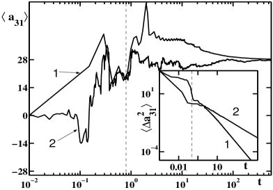
Figure 1: Examples of convergence of the coefficient $a_{31}$ corresponding to parameter $r$ of the Lorenz system (13) for the total length of the time record $T=560$ and the following sets of parameters: line $1$ $\{d_{n}\}=\{0.01,0.012,0.014\}$ time step $h=0.002$; line $2$ $\{d_{n}\}=\{100,120,140\}$ and $h=0.00002$. The insert shows dispersion $\langle\Delta a_{31}^{2}\rangle$=$\langle a_{31}^{2}\rangle$ - $\langle a_{31}\rangle^{2}$ for the same sets of parameters. The vertical dashed line shows the time-scale of the step-wise decrease in the variance.

We found a step-wise decrease in variances that occurs on a time scale of the period of oscillations $\tau_{osc}\approx 0.6$ (dashed line in the figure). The error of the inference is sensitive to the noise intensity, total time $T$ and the time step $h$. For example, for the parameters of the curve 1 in the Fig. 1 the relative error was $0.015\%$. The ratio $T/h$ has to be increased at least 250 times to achieve error less then $1\%$ when the noise intensity is increased $10^{4}$ times (curve 2 in the figure).

Finally, we apply our method to study the stochastic nonlinear dynamics of complex physiological system. To be specific we infer the strength, directionality and a degree of randomness of the cardiorespiratory interaction from the central venous blood pressure signal (record 24 of the MGH/MF Waveform Database available at www.physionet.org). Such estimations provide valuable diagnostic information about the responses of the autonomous nervous system Hayano:03 ; Malpas:02 . However, it is inherently difficult to dissociate a specific response from the rest of the cardiovascular interactions and the mechanical properties of the cardiovascular system in the intact organism Jordan:95 . Therefore a number of numerical techniques were introduced to address this problem using e.g. linear approximations Taylor:01 , or semi-quantitative estimations of either the strength of some of the nonlinear terms Jamsek:03 or the directionality of coupling Rosenblum:02 ; Palus:01 . But the problem remains wide open because of the complexity and nonlinearity of the cardiovascular interactions. Our algorithm provides an alternative effective approach to the solution of this problem. To demonstrate this we use a combination of low- and high-pass Butterworth filters to decompose the blood pressure signal into 2-dimensional time series $\{{\bf s}(t_{k})=(s_{0}(t_{k}),s_{1}(t_{k})),\,\,t_{k}=kh,\,k=0:K\}$ representing observations of mechanical cardiac and respiratory degrees of freedom on a discrete time grid with step $h=0.002$ sec. We now introduce an auxiliary two-dimensional dynamical system whos trajectory ${\bf x}(t)=(x_{0}(t),x_{1}(t))$ is related to the observations $\{{\bf s}(t_{k})\}$ as follows

$$x_{n}(t_{k})=a_{1n}\,\frac{s_{n}(t_{k}+h)-s_{n}(t_{k})}{h}+a_{2n}s_{n}(t_{k})+a_{3n},$$

where $n=0,1$. The corresponding simplified model of the nonlinear interaction between the cardiac and respiratory limit cycles has the form (cf. with  Stefanovska:01a )

$$\dot{x}_{n}=b_{1n}+b_{2n}s_{n}+b_{3n}x_{n}+b_{4n}s_{n}^{2}+b_{5n}x_{n}^{2}+b_{6n}s_{n}x_{n}$$

$$+\,b_{7n}s_{n}^{3}+b_{8n}s_{n}^{2}x_{n}+b_{9n}x_{n}x_{n}^{2}+b_{10n}x_{n}^{3}+b_{11n}x_{n}x_{n-1}$$

$$+\,b_{12n}x_{n}^{2}x_{1-n}+b_{13n}x_{n}x_{1-n}^{2}+\xi_{n}(t),\quad n=0,1.$$ (15)

where $\xi_{n}(t)$ is a Gaussian white noise with correlation matrix $D_{n\,n^{\prime}}$ (3). We emphasize that a number of important parameters of the decomposition of the original signal (including the bandwidth, the order of the filters and the scaling parameters $a_{ki}$) have to be selected to minimize the cost (7) and provide the best fit to the measured time series $\{{\bf s}(t_{k})\}$. The parameters of the model (15) can now be inferred directly from the noninvasively measured time series of blood pressure. The comparison between the time series of the inferred and actual cardiac oscillations is shown in Fig. 2.

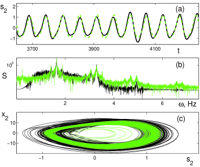
Figure 2: (a) Time series of the cardiac oscillations $s_{2}(n)$ in arbitrary units (black line) obtained from central venous blood pressure with 4-th order Butterworth filter (low-and high- cut-off frequencies were $f_{l}=0.8Hz$ and $f_{h}=2.8Hz$ and the sample rate was 90 Hz after resampling of the original signal). Inferred time series of the cardiac oscillator (green line). (b) Power spectrum of the cardiac oscillations obtained from the real data (black line). Power spectrum of the inferred oscillations (green line). (c) Limit cycle of the cardiac oscillations $(x_{2}(n),y_{2}(n)$ obtained from real data as described in the text (black line). Limit cycle of inferred oscillations (green line).

Similar results are obtained for the respiratory oscillations. In particular, the parameters of the nonlinear coupling and of the noise intensity of the cardiac oscillations are $b_{112}=3.9,b_{122}=0.62$, $b_{132}=-13.4$, and $D_{22}=4.75$ ($\langle\xi^{2}_{y_{2}}(t)\rangle=D_{22}$). Consistent with expectations, in all experiments the parameters of the nonlinear coupling are two orders of magnitude higher for the cardiac oscillations as compared to their values for the respiratory oscillations reflecting the fact that respiration strongly modulates cardiac oscillations, while the opposite effect of the cardiac oscillations on respiration is weak. Remarkably, our technique infers simultaneously the strength, directionality of coupling and the noise intensities in the cardiorespiratory interaction directly from the non-invasively measured time series.

In conclusion, we have derived an efficient technique for recursive inference of dynamical model parameters that does not require extensive numerical optimization and provides optimum compensation for the dynamical noise-induced errors. We verified the robustness of the technique in a very broad range of parameters of dynamical models, using synthetic data from the chaotic noise-driven Lorenz system. Successful application of the technique to inference from real data of the nonlinear interaction between the cardiac and respiratory oscillations in the human cardiovascular system is particularly encouraging, as it opens up a new avenue for the Bayesian inference of strongly nonlinear and noisy dynamical systems with limited first-principles knowledge. Future extensions will include more realistic observation schemes with “hidden” variables and finite measurement noise.

This work was supported by NASA IS IDU project (USA) and by EPSRC (UK).

References

- (1) M.B.Willemsen, et al., Phys. Rev. Lett. 84, p.4337 (2000).
- (2) K. Visscher, et al., Nature 400, p.184 (1999).
- (3) D.J.D. Earn, et al., Science, 287, p.667 (2000).
- (4) J.Christensen-Dalsgaard, Rev. Mod. Phys., 74, 1073 (2002).
- (5) H. Kantz and T. Schreiber, Nonlinear Time Series Analysis (Cambridge Univ. Press, Cambridge, UK, 1997).
- (6) P. McSharry, L. Smith, Phys. Rev. Lett. 83, 4285 (1999).
- (7) J.P.M. Heald, J. Stark, Phys. Rev. Lett. 84, 2366 (2000).
- (8) R. Meyer, N. Christensen, Phys. Rev. E 62, 3535 (2000).
- (9) J. Gradisek et al., Phys. Rev. E 62, 3146 (2000).
- (10) R. Meyer, N. Christensen, Phys. Rev. E 65, 16206 (2001).
- (11) J.-M. Fullana, M. Rossi, Phys. Rev. E 65, 31107 (2002).
- (12) M. Siefert et al., Europhys. Lett. 61, 466 (2003).
- (13) R. Graham, Z. Phys. B 26, 281 (1977).
- (14) M.I. Dykman, Phys. Rev. A 42, 2020 (1990).
- (15) In general, the posterior PDF is characterized by an inverse joint covariance matrix for the model parameters and . Elements of are given by the corresponding second derivatives of (7) with respect to , . The matrix should be recursively updated along with and after processing each block of data. Our algorithm only involves the part of corresponding to elements of (given by ). The rest of the matrix elements of was zeroed out. This shortcut does not change the algorithm preformance in the case under study where the time step is sufficiently small and elements of are typically inferred from fewer data points as compared to the components of the vector .
- (16) S. C. Malpas, Am. J. Physiol.: Heart. Circ. Physiol. 282, H6 (2002).
- (17) J. Hayano and F. Yasuma, Cardiov. Res. 58, 1 (2003).
- (18) D. Jordan, in Cardiovascular regulation, edited by D. Jordan and J. Marshall (Portland Press, Cambridge, 1995).
- (19) J. A. Taylor et al., Am J Physiol Heart Circ Physiol 280, H2804 (2001).
- (20) J. Jamsek, A. Stefanovska, P.V.E. McClintock, I.A. Khovanov, Phys. Rev. E, 68, 016201 (2003)
- (21) M. G. Rosenblum et al., Phys. Rev. E. 65, 041909 (2002).
- (22) M. Palus, A. Stefanovska, Phys. Rev. E, 67, 055201 (2003)
- (23) A. Stefanovska, et al., Physiol. Meas. 22, 535 (2001); A. Stefanovska, et al., Physiol. Meas. 22, 551 (2001).