Ballistic trajectory: parabola, ellipse, or what?

Abstract

Mechanics texts tell us that a particle in a bound orbit under gravitational central force moves on an ellipse, while introductory physics texts approximate the earth as flat, and tell us that the particle moves in a parabola. The uniform-gravity, flat-earth parabola is clearly meant to be an approximation to a small segment of the true central-force/ellipse orbit. To look more deeply into this connection we convert earth-centered polar coordinates to “flat-earth coordinates” by treating radial lines as vertical, and by treating lines of constant radial distance as horizontal. With the exact trajectory and dynamics in this system, we consider such questions as whether gravity is purely vertical in this picture, and whether the central force nature of gravity is important only when the height or range of a ballistic trajectory is comparable to the earth radius. Somewhat surprisingly, the answers to both questions is “no,” and therein lie some interesting lessons.

I Introduction

The trajectory of a particle moving without drag under the influence of the gravitational field of a perfectly spherical earth is a conic section. Since a cannonball, for example, is on a bound orbit, its flight from muzzle to target is part of an ellipse, as shown on the left in Fig. 1. The center of the earth is at the (distant) focus of the highly eccentric ellipse, and the part of the ellipse relevant to cannonball flight is a small segment near the apogee. Introductory texts, however, treat ballistic motion using Galileo’s approach. Specifically, the horizontal and vertical components of the motion of the projectile are separated, and the trajectory is given by a parabola. The parabola as a limit of an ellipse was noted by Newton in the Principiaprincipia :

If the ellipsis, by having its centre removed to an infinite distance, degenerates into a parabola, the body will move in this parabola; and the force, now tending to a centre infinitely remote, will become equable. Which is Galileo’s theorem.

Many of the introductory textbooks we have reviewed do not discuss the nature of the approximation, i.e., they do not discuss the conditions under which the flat-earth parabola is an accurate approximation for what is really a central force ellipse. Some textbooks, however, do make explicit statements about the approximation, statements that seem plausible, but turn out to be incorrect. Specifically, we found three classes of conditions which are used in those textbooks that do discuss the validity of the approximation. In the first class it is assumed that the maximal height of the trajectory above the surface of the earth is small compared with the radius of the earth (or, equivalently, that the magnitude of the gravitational acceleration does not change by much along the trajectory)height ; in the second class it is assumed that the range of the trajectory is small compared with the radius of the earth (or, equivalently, that the direction of the gravitational acceleration does not change by much along the trajectory)range ; in the third class it is assumed that both the height and the range are small compared with the radius of the earth (both the magnitude and the direction of the gravitational acceleration do not change by much)height_and_range . Other textbooks refer vaguely to neglecting the curvature of the earth in justifying the approximation, but do not quantify the condition vague .

In this paper we show that the correct condition under which the flat-earth picture is a good approximation for the trajectory, is that the maximal curvature of the trajectory is much greater than the curvature of the surface of the earth. This condition coincides with the three classes of naive conditions for many, but not all, trajectories. There are trajectories for which all the three naive classes of conditions are satisfied, but for which the approximation fails to be valid.

To “flatten the earth” without any approximation, we introduce geocentric polar coordinates $r,\phi$ in the plane of the orbit (as shown on the left of Fig. 1) and we plot them (on the right in Fig. 1) as if they were Cartesian coordinates $x,y$. We let $R$ denote the radius of our perfect earth, and we take $h$ to be the height, above the earth, of the peak of the trajectory. The apogee of the particle orbit is then at a distance $r=R+h$ from the center of the earth. For convenience, we choose our zero of $\phi$ so that it coincides with the apogee of the orbit.

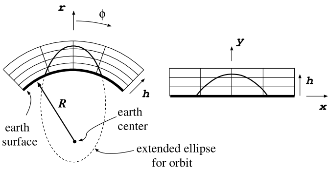
Figure 1: Ellipse for a ballistic trajectory pictured in polar coordinates and in flat earth coordinates.

In order to view the space above the earth in this way, as if the earth were flat, we need to distort the coordinates in somewhat the same manner as a map maker. We choose to do this with the explicit relationship notunique

$$x=(R+h)\phi\quad\quad\quad\quad y=r-R\ .$$ (1)

and to plot $x,y$ as if they were Cartesian coordinates.

In this paper we shall focus on two questions about exact ballistic trajectories. The first is the accuracy of the parabolic approximation. The naive expectation of most students (and many teachers) is that the approximation is valid if the trajectory is “small” compared to the radius of the earth, i.e. , if neither $h$ nor the range of the trajectory is comparable to the earth radius $R$. We shall see that this naive expectation is too naive.

Our second question involves the vertical nature of gravitation. In the “true” picture of gravitational acceleration, on the left side of Fig. 1, the gravitational force is radially directed towards the center of the earth. These radial lines are converted to vertical lines by the redrawing of the coordinates on the right hand side of Fig. 1, and by the transformation in Eq. (1). It would seem, therefore, that gravitational acceleration must be acting vertically in the picture on the right hand side of Eq. (1). The introductory textbooks add to this the assumption that $g$ is constant, and prove that a particle being acted upon only by gravitational forces moves in a parabola. This argument leads unavoidably to the conclusion that the particle trajectory deviates from a parabola only due to the slight variation of $g$ with altitude. We shall see that again the naive expectation is not correct.

II Elliptical orbits in flat-earth coordinates

To describe the orbit of a unit mass particle we start by letting

$$L=r^{2}\frac{d\phi}{dt}$$

represent the particle angular momentum per unit particle mass. With standard techniquesanymechbook we can write the equation of the particle’s orbit, in polar coordinates, as

$$r=\frac{1}{\frac{GM}{L^{2}}+\left(\frac{1}{R+h}-\frac{GM}{L^{2}}\right)\cos{\phi}}\ ,$$ (2)

which is the equation of an ellipse (though not in the most familiar form). Here $M$ is the mass of the earth and $G$ is the universal gravitational constant.

We can convert Eq. (2) to the flat-earth picture simply by introducing the $x,y$ coordinates of Eq. (1), and can write the trajectory in the right hand side of Fig. 1 as

$$y+R=\frac{1}{\frac{GM}{L^{2}}+\left(\frac{1}{R+h}-\frac{GM}{L^{2}}\right)\cos{(x/[R+h])}}\ .$$ (3)

To simplify the complex appearance of this equation we introduce two dimensionless parameters. The first is $\epsilon\equiv h/R$, a parameter that tells us something about the relative size of the trajectory and the earth. We want our second parameter to be expressed in terms of quantities appropriate to the usual description of a ballistic trajectory. To that end we introduce the parameter $V_{horiz}$, the particle velocity at the top of the trajectory, and we combine it with the acceleration of gravity at the surface of the earth $g$ to form the dimensionles parameter

$$\alpha\equiv\frac{V^{2}_{horiz}}{gh}\ .$$ (4)

We next note that $V_{horiz}=L/(R+h)$ and $g=GM/R^{2}$, so that $\alpha$ is equivalent to $(L^{2}/GMh)/(1+\epsilon)^{2}$. With these equivalences we can rewrite the trajectory in Eq. (3) as

$$\frac{y}{h}=\frac{\alpha(1+\epsilon)^{2}}{1+\left[\alpha\epsilon(1+\epsilon)-1\right]\cos{\left(\frac{\epsilon(x/h)}{[1+\epsilon]}\right)}}-\frac{1}{\epsilon}\ .$$ (5)

In Eq. (5), the only length scale that explicitly appears is $h$, a scale appropriate to the description of ballistic trajectories. But the parameter $\epsilon\equiv h/R$ still carries information about the size of the earth. The familiar parabolic trajectory follows when this parameter is taken to be very small. To see this, we can expand the right hand side in powers of $\epsilon$ and keep only the term to zero order in $\epsilon$ (keeping $\alpha$ fixed). The result is

$$\frac{y}{h}=1-\frac{1}{2\alpha}\frac{x^{2}}{h^{2}}=1-\frac{g}{2V^{2}_{horiz}}\frac{x^{2}}{h}\ ,$$ (6)

the standard parabolic ballistic trajectory,

We now look more carefully at the exact orbit in the flat-earth coordinates of Eq. (5). In Fig. 2 we present trajectories for $\epsilon=10^{-4}$, hence for $h\approx 0.63$ km. The derivation above, of the parabolic approximation, assumes that $\alpha$ is of order unity. To see interesting deviations from a parabola, we consider large values of $\alpha$ in the figure. For $\alpha=15,000$, the deviations from the parabola are striking indeed; the trajectory bends upward. This, of course, is simply the appearance in our coordinates of an elliptical orbit for which the radius of curvature at the apogee is greater than the radius of curvature of the earth’s surface.

Figure 2:

Trajectories for $h/R=10^{-4}$. Solid curves are exact trajectories in flat-earth coordinates and dashed curves are parabolic approximations. Curves are labeled by the value of $\alpha$ to which they correspond.

What may be most surprising in Fig. 2, is that large deviations from the parabola occur when the range of a trajectory is only around $90h$, or about 60 km, a tiny distance compared to the size of the earth. To see why this is so, we can put $y=0$ in Eq. (5) and we can solve for $x$, half the range of the particle:

$$\frac{x}{h}=\frac{1+\epsilon}{\epsilon}\cos^{-1}{\left(\frac{1-\epsilon\alpha(1+\epsilon)^{2}}{1-\epsilon\alpha(1+\epsilon)}\right)}=\sqrt{2\alpha}\left[1+\frac{\epsilon}{2}(\alpha-1)\right]+{\cal O}\left(\epsilon^{2}\right)\ .$$ (7)

The fractional error in the range of the trajectory, for large $\alpha$ is therefore

$$\frac{\epsilon}{2}(\alpha-1)\approx\frac{\epsilon\alpha}{2}\approx\frac{{\rm range}^{2}}{16Rh}\ ,$$ (8)

where we have used the fact that the range is approximately $2h\sqrt{2\alpha}$. Equation (8) shows that the deviation from the standard range formula is large when the range is of order $\sqrt{Rh}$ or $R\sqrt{\epsilon}$, and hence can be important for orbits that are much smaller than the scale of the earthloworbit . This conclusion is in good agreement with the $\alpha=3000,\epsilon=10^{-4}$ example in Fig. 2. For these parameters the parabolic approximation misses the target by $15\%$.

There is a nice way of understanding what we have just found. The replacement of the spherical earth surface with a flat surface, in Fig. 1, is justifiable only if the trajectory is more sharply curved than is the earth surface. That is, if the minimal radius of curvature along the trajectory is smaller than the radius of the earth. The radius of curvaturecurvature ${\cal R}$ of the trajectory iscurvature_ellipse

$${\cal R}:=\frac{\left[1+(dy/dx)^{2}\right]^{3/2}}{\left|d^{2}y/dx^{2}\right|}=\frac{h\alpha}{\left[1+x^{2}/\left(h\alpha\right)^{2}\right]^{3/2}}\ ,$$ (9)

where we have used Eq. (6). The condition that the maximum curvature of the trajectory (the curvature at $x=0$) is much greater than the curvature of the earth’s surface is that $h\alpha/R\ll 1$. This is violated when $\epsilon\alpha\sim 1$ for which we have, from Eq. (8), a large deviation from the parabolic range prediction. We can now understand this in terms of radius of curvature of the trajectory. For a small $h$, high velocity orbit, a projectile can move “just above” the surface of the earth on a trajectory with a range much larger than its height $h$ (but much smaller than $R$). The curvature of that trajectory in space is mostly due to the curvature of the earth. In the flat earth picture the true trajectory would seem to have almost constant height, and would greatly deviate from a parabolalatus_rectum . It should be noted that the meaning of a flat earth trajectory disappears if $\epsilon\alpha>1$. It follows from Eq. (9) that for $\epsilon\alpha>1$ the radius of curvature at the apogee exceeds that of the earth. This suggests that the elliptical or hyperbolic trajectory of the projectile will not intersect the earth surface. That this is, in fact, true can be verified by looking for solutions of $y=0$ in Eq. (5); for $\epsilon\alpha>1$, there are no solutions with positive $\epsilon$.

There is also an interesting non-geometrical way of viewing the condition $\alpha\epsilon\ll 1$. From the definitions of $\alpha$, $\epsilon$, and $g$, we have

$$\alpha\epsilon=\frac{V^{2}_{horiz}}{gR}=\frac{V^{2}_{horiz}}{V^{2}_{circ}}=\frac{2V^{2}_{horiz}}{V^{2}_{esc}}\,,$$ (10)

where $V_{circ}$ is the velocity of a circular orbit with radius $R$ (i.e. , just above the earth surface), and $V_{esc}$ is the escape velocity from the earth surface. The condition $\alpha\epsilon\ll 1$, then, is simply the condition that the motion is very slow compared to typical “orbital” (as opposed to “trajectory”) motions. For trajectories with $V_{horiz}$ comparable to $V_{esc}$ we should not be surprised that the deviation from a parabolic projectile trajectory is significant. We may, however, be surprised that the range of that trajectory may be short, much less than the earth radius. The key idea here is that the range is kept short by imposing a small value of $h$. For sufficiently small values of $h$ the high velocity projectiles hit the earth’s surface before they get a chance to show how far they would have gone in their large elliptical orbits. In order for this to happen, in order for the range to be kept small, the value of $h$ must be reduced as $V_{horizon}$ is increased. The limiting case is $V_{horizon}=V_{esc}/\sqrt{2\;}$, the maximum for which the trajectory has a range (i.e., for which the trajectory intercepts the earth’s surface). As this limit is approached, the condition on $h$, for the range to be much less than the earth radius, is $\epsilon\ll\left[1-2(V_{horizon}/V_{esc})^{2}\right]$.

III Is gravity vertical in the flat-earth picture?

In Section I we argued that gravitational acceleration must be vertical in the flat earth picture. It is apparent in Fig. 2 that this cannot be correct. For the $\alpha=15,000$ trajectory, the particle is accelerating upward. And this particle is at a height of only a kilometer or so above the earth’s surface, where the acceleration of gravity is certainly close to 9.8 m/sec² and is even more certainly downward.

Another clear indication that “vertical acceleration” is not the whole story, is the fact that the horizontal velocity $dx/dt$ changes in time. Figure 3 shows the small, but nonzero, fractional change in the horizontal velocity along the orbit.

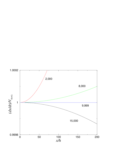
Figure 3:

Trajectories for $h/R=10^{-4}$. The horizontal velocity $dx/dt$ is shown as a function of horizontal position $x$. ($V_{horiz}$ is the horizontal velocity at the apogee.) Curves are labeled by $\alpha$. The value $\alpha=9,999$ represents a circular orbit.

To understand the results in this figure we note that

$$\frac{1}{V_{horiz}}\frac{dx}{dt}=\frac{(R+h)}{V_{horiz}}\frac{d\phi}{dt}=\frac{(R+h)L}{V_{horiz}r^{2}}=\frac{(R+h)^{2}}{r^{2}}\ .$$ (11)

In this simple calculation it is easy to see why the horizontal velocity changes: it is proportional to $L/r^{2}$. The angular momentum $L$ is constant, but $r$ is not constant except in the case of the circular orbit for which $\alpha=\alpha_{crit}\equiv R^{2}/h(R+h)$. As the particle moves to smaller radius (in the case $\alpha<\alpha_{crit}$) the horizontal velocity must increase; as the particle moves to larger radius (in the case $\alpha>\alpha_{crit}$) the particle velocity must decrease. In this mathematics it is easy to see why the horizontal velocity changes during the motion.

At a deeper level, the failure of naive intuition is due to the tacit expectation that the equations of motion for a unit mass particle can be put in a form

$$\frac{d^{2}x}{dt^{2}}=F_{x}\quad\quad\quad\frac{d^{2}y}{dt^{2}}=F_{y}\,,$$ (12)

where $F_{x}$ and $F_{y}$ are only functions of position $x,y$. Since particles released from rest will fall vertically downward we conclude that $F_{x}=0$, and gravity is vertical.

We are misled to this conclusion by the Cartesian appearance of the $x,y$ coordinates on the right side of Fig. 1. The actual equations of motioneqsofmotion , turn out to be

$$\frac{d^{2}x}{dt^{2}} = -\frac{2}{(y+R)}\frac{dx}{dt}\frac{dy}{dt}$$ (13)

$$\frac{d^{2}y}{dt^{2}} = -\frac{GM}{(y+R)^{2}}+\frac{(y+R)}{(R+h)^{2}}\left(\frac{dx}{dt}\right)^{2}\,.$$ (14)

In the case of a vertical trajectory ($dx/dt=0$) the equations are in complete agreement with our expectations. When $dx/dt\neq 0$, however, the velocity dependent terms, absent in Eqs. (12), are responsible for the failure of intuitonnotG ; neglect_vel . These velocity dependent terms are due to the fact that the $x,y$ coordinate lines are actually curved lines through physical space. We can draw them as straight lines, but the way in which we draw them, or the symbols we use to represent them, do not change the fact that they are curved in physical space. This curvature of spatial coordinates comes with its usual kinematical consequences. The $(dx/dt)^{2}$ in Eq. (14), for example, is just the usual centripetal term disguised by unusual coordinate names.

IV Conclusions

It is plausible to expect that the uniform-gravity, flat-earth gravity parabola is an accurate approximation if the height $h$ of the trajectory, and the range of the trajectory, are both much less than the earth radius $R$. In terms of our parameterization these conditions are, respectively $\epsilon\ll 1$ and $\alpha\epsilon^{2}\ll 1$. If we are to have the kinematics correct, as well as the shape of the orbit, then clearly the first condition is necessary; if $h$ is not small compared to $R$ gravity cannot be of uniform strength.

The second condition, however, is not sufficiently strict. The correct second condition for the validity of the flat-earth approximation is that the maximum curvature of the trajectory be much greater than the curvature of the earth’s surface. In our notation this corresponds to orbits that satisfy $\alpha\epsilon\ll 1$. This condition is not satisfied for a class of trajectories that do satisfy $\epsilon\ll 1$ and $\alpha\epsilon^{2}\ll 1$. That class consists of low height, high velocity motions. The importance of the high velocity feature of these orbits can be seen in the fact that our condition $\alpha\epsilon\ll 1$ is equivalent to the condition that the velocity of the orbit is much less the escape velocity from the earth surface.

V Acknowledgment

We thank Benjamin Bromley for pointing out the low-velocity interpretation, given in Eq. (10), for the parabola condition. This work has been partially supported by the National Science Foundation under grant PHY0244605.

References

- (1) I. Newton, The Principia, translated by A. Motte (Prometheus Books, New York, 1995), Scholium following Proposition X of Book I, Section II. Newton does not give much details about how the limit should be taken. While taking the center of the ellipse to infinity and letting the eccentricity approach unity (from below), the latus rectum is to be kept fixed. Notice that the center of the earth, at the distant focus, is also taken to infinity. For more details on a closely related way to take the limit see S. Chandrasekhar, Newton’s Principia for the Common Reader (Oxford University Press, Oxford, 1995).
- (2) K.R. Symon, Mechanics (Addison-Wesley, Reading, MA, 1971), pp. 111-112. This is a more advanced-level textbook (not introductory!), which also discusses the complicated issue of how the changing resistance of air with altitude affects the trajectory, but only discusses the height as a condition for the trajectory to be parabolic in the absence of air resistance.
- (3) I.M. Freeman, Physics: Principles and Insights (McGraw Hill, New York, 1973), p. 107; R. Wolfson and J.M. Pasachoff, Physics, 3rd ed (Addison Wesley, Reading, MA, 1999), Vol. 1, p. 72; R.A. Serway, Principles of Physics (Saunders, Orlando, FL, 1994), P. 63; D.E. Roller and R. Blum, Physics (Holden-Day, San Francisco, CA, 1981), vol. 1, p. 76, and p. 346.
- (4) D.C. Giancoli, Physics for Scientists & Engineers with Modern Physics, 3rd ed. (Prentice Hall, Upper Saddle River, NJ, 2000), p. 56; S. M. Lea and J.R. Burke, Physics: The Nature of Things (Brooks/Cole, St. Paul, MN, 1997), p. 92. The last reference also explicitly addresses the parabolic vs. elliptic trajectories.
- (5) E. Hecht, Physics Calculus (Brooks/Cole, Pacific Grove, CA, 1996), p. 94.
- (6) Our choice is not the only reasonable way of carrying out this mapping. We could alternatively have chosen , for example. By comparison, our choice suffers from having unequal physical distances, for equal increments of , along coordinate lines. Our choice, however, gives much simpler dynamical equations at the end of this article. The choice made has no distinguishable effect on the appearance of the results given in the figures.
- (7) See, e.g., J. B. Marion and S. T. Thornton, Classical Dynamics of Particles and Systems, 4th ed. (Saunders, Fort Worth, TX, 1995); H. Goldstein, C. P. Poole, and J. L. Safko, Classical Mechanics, 3rd ed. (Pearson, Upper Saddle River, NJ, 2001).
- (8) This sort of high velocity motion is not typical of practical ballistic trajectories, in which projectiles are launched at an angle near 45o. For such trajectories is of order unity, and the parabolic approximation is accurate. For a given range and a given , a larger value of means a larger value of , or equivalently of the required muzzle velocity. Though the conclusion from Eq. (8) is meant to be a point of principle, not of practical importance, it is interesting that large guns exist that are able to achieve muzzle velocities of several km/sec necessary to have peak height and range, of the same order as the values km and range km in our example.
- (9) The radius of curvature at a point in a plane curve is defined as the radius of the “osculating circle,” or the circle of curvature, the circle whose first and second derivative agree with those of the curve at that point. This curvature is equivalent to the magnitude of the derivative, with respect to arc length, of the unit tangent to the curve. See, e.g., M. P. do Carmo, Differential Geometry of Curves and Surfaces (Prentice Hall, Upper Saddle River, NJ, 1976).
-
(10)
The radius of curvature of the ellipse at its
apogee is
For (which is equivalent to ), and for , this coincides with Eq. (9) at the apogee. - (11) The condition that the parabolic trajectory is a good approximation for the true orbit, i.e., that , is equivalent to , being the semilatus rectum.
- (12) These equations can be derived by substituting and in the standard equations for central force motion. A rather simpler equivalent set of equations follows, of course, by writing the two constants of motion, energy and angular momentum, in terms of coordinates. The form in Eq. (14), with second derivatives with respect to time, is given to emphasize the velocity dependence of the acceleration.
- (13) One could claim that we have not shown that “gravity” fails to be vertical. The velocity-dependent terms in Eqs. (14), after all, do not contain the gravitational constant . Those terms are actually kinematic terms due to the nature of the coordinates. To avoid this criticism, the fallacious argument at the end of Sec. I was made for “a particle being acted upon only by gravitational forces.”
- (14) Notice that the velocity dependent term on the right hand side of Eq. (14) is made negligible with respect to the term not depending on the velocity if , but one cannot neglect the velocity dependent right hand side of Eq. (13). Notice, however, that typically indeed and the right hand side of Eq. (13) is rather small, such that Galileo’s picture of separate horizontal and vertical motions is a fair description of the motion. However, for the values of the parameters we considered above, is about unity, such that it is easy to see that the equations of motion (13) and (14) are indeed coupled, and “gravity is not vertical.”