Exact vortex solution of the Jacobs-Rebbi equation for ideal fluids

Abstract

The Jacobs-Rebbi equation arises in many contexts where vortical motion in two-dimensional ideal media is investigated. Alternatively, it can be derived in the Abelian Higgs field theory. It is considered non-integrable and numerical solutions have been found, consisting of localised, robust vortices. We show in this work that the equation is integrable and provide the Lax pair. The exact solution is obtained in terms of Riemann theta functions.

1 Introduction

Studying the interaction energy of vortices of the Ginsburg-Landau model of superconductivity, Jacobs and Rebbi [1] have derived a nonlinear equation from which the scalar function (order parameter) can be calculated. The derivation is based on the similarity of this model with the Abelian Higgs theory [2], [3], [4]. In a special case, corresponding to a particular choice of parameters, the nonlinear equation takes a simple form, a nonlinear elliptic differential equation in two spatial dimensions. The same problem is treated by Dunne [5] in a general context of gauge theories with Maxwell and/or Chern-Simons terms in the Lagrangean density. The same Abelian Higgs field theory is discussed and the special case mentioned above is identified as the minimum of the action functional (saturation of the Bogomolnyi inequality), realized by fields obeying a simpler set of equations. This special case is called self-duality, with reference to the equality of the differential two-form (the curvature of the fibre bundle) with its Hodge dual in the geometrical setting of the field-theoretical content.

In fluids and plasmas coherent motion and in particular vortices are ubiquituous [6]. They can appear even in turbulent states. In two-dimensions, apart from the dynamical equations derived from the conservation laws an alternative model has been proposed, consisting of the motion of discrete, point-like vortices in plane interacting via a potential [7]. It has been shown that this model can be mapped onto a field-theoretical model whose structure is very similar with the non-Abelian gauge-Higgs field theory [8]. The self-dual state of this field at stationarity is precisely the asymptotic state of the ideal fluid, which effectively provides an analytic derivation of the sinh-Poisson equation describing the fluid streamfunction. For the stationary states attained at very large time by the ideal ion instability in plasma (described by Hasegawa-Mima), the model of discrete vortices interacting in plane introduces a short-range potential (then a massive photon of the gauge field in the field theoretical model).

There are two differences between the field theoretical models developed starting from the plasma problems and the model from which Jacobs-Rebbi equation is derived. First, the absolute value of the scalar Higgs field is constant at large distances (on a circle of very large radius); this means that the vorticity should be constant at large distance, in the plasma case. Second, the model must be Abelian, which is less than we would need for treating the case of the Euler fluid (the sinh-Poisson equation). However, there are physical situations where the boundary conditions for the vorticity are compatible with the formulation of the Jacobs-Rebbi model. And, it is known that Abelian models can provide description of plasma problems (guiding centre particles, for example) leading to the Liouville equation. The effect of these differences still needs to be investigated, but in any case, the exact determination of the solution can only be a useful instrument.

It is usual to consider that the Jacobs-Rebbi equation cannot be solved analytically and in consequence numerical solutions have been provided.

We show in this paper that the Jacobs-Rebbi equation is exactly integrable. We consider the integrability on periodic domains and provide the Lax pair. We follow the standard algebraic-geometric method of integration and generate explicit solutions in terms of Riemann theta functions.

2 Derivation of the Jacobs-Rebbi equation

2.1 Derivation in the context of Ginsburg-Landau theory

The Ginsburg-Landau theory is the framework in which the Jacobs-Rebbi equation has been derived, since the original aim was the investigation of the energy of interaction between two vortices in superconducting Helium. The interest for vortical structures of Ginsburg-Landau comes also from the observation that the theory of a gauge field coupled to a scalar field (Abelian Higgs field) can in some cases exhibit also coherent vortical structures. We include in this Section the derivation according by Jacobs and Rebbi [1]. In fluid physics other approaches can be developed to arrive at similar forms of the equation.

The free energy of the Ginsburg-Landau theory and the potential energy of the Abelian-Higgs theory is

$$E = \int d^{3}x\left\{\frac{1}{4}F_{ij}F^{ij}\right.$$

$$\left.+\frac{1}{2}\left|\left(\partial_{i}-ieA_{i}\right)\phi\right|^{2}+c_{4}\left(\left|\phi\right|^{2}-c_{0}^{2}\right)^{2}\right\}$$

where $\phi$ is a complex scalar field, $A_{i}$ is the Abelian gauge potential and

$$F_{ij}=\partial_{i}A_{j}-\partial_{j}A_{i}$$

The minimum of the energy is attained for

$$\left|\phi\right|=c_{0}\neq 0$$

The variables are rescaled as

$$x_{i}=\frac{1}{c_{0}e}\widetilde{x}_{i}$$

$$A_{i}=c_{0}\widetilde{A}_{i}$$

$$\phi=c_{0}\widetilde{\phi}$$

and the energy becoms

$$E = \frac{c_{0}}{e}\int d^{3}\widetilde{x}\left\{\frac{1}{4}\widetilde{F}_{ij}\widetilde{F}^{ij}\right.$$

$$\left.+\frac{1}{2}\left|\left(\widetilde{\partial}_{i}-ie\widetilde{A}_{i}\right)\widetilde{\phi}\right|^{2}+\frac{\lambda^{2}}{8}\left(\left|\widetilde{\phi}\right|^{2}-1\right)^{2}\right\}$$

where

$$\lambda^{2}=\frac{8c_{4}}{e^{2}}$$

The model is restricted to the case where all field functions does not depend on the third coordinate and

$$A_{3}\equiv 0$$

In plane the coordinates are expressed by complex variables

$$z = \widetilde{x}_{1}+i\widetilde{x}_{2}$$

$$\overline{z} = \widetilde{x}_{1}-i\widetilde{x}_{2}$$

and the differential operators can be defined

$$\partial \equiv \frac{1}{2}\left(\frac{\partial}{\partial\widetilde{x}_{1}}-i\frac{\partial}{\partial\widetilde{x}_{2}}\right)$$

$$\overline{\partial} \equiv \frac{1}{2}\left(\frac{\partial}{\partial\widetilde{x}_{1}}+i\frac{\partial}{\partial\widetilde{x}_{2}}\right)$$

Analoguous combinations are used for the two remaining potential components

$$A = \frac{1}{2}\left(\widetilde{A}_{1}-i\widetilde{A}_{2}\right)$$

$$\overline{A} = \frac{1}{2}\left(\widetilde{A}_{1}+i\widetilde{A}_{2}\right)$$

The energy per unit length along the coordinate axis $x_{3}$ is

$$E=\frac{c_{0}\pi}{e}\mathcal{E}$$

$$\mathcal{E} = \frac{1}{2\pi}\int dzd\overline{z}\left\{2\left|\overline{\partial}A-\partial\overline{A}\right|\right.$$

$$\left.+\left|\left(\partial-iA\right)\widetilde{\phi}\right|^{2}+\left|\left(\overline{\partial}-i\overline{A}\right)\widetilde{\phi}\right|^{2}+\frac{\lambda^{2}}{8}\left(\left|\widetilde{\phi}\right|^{2}-1\right)^{2}\right\}$$

In the following the tilda will be omitted.

The equations of motion that are derived from the Lagrangean

$$\left(\partial-iA\right)\left(\overline{\partial}-i\overline{A}\right)\phi+\left(\overline{\partial}-i\overline{A}\right)\left(\partial-iA\right)\phi-\frac{\lambda^{2}}{4}\phi\left(\left|\phi\right|^{2}-1\right)=0$$

$$4\partial\overline{\partial}A-4\partial^{2}A$$

$$-i\overline{\phi}\partial\phi+i\phi\partial\overline{\phi}$$

$$-2A\phi\overline{\phi}$$

$$= 0$$

For a general value of $\lambda$ one can replace particular forms for the two functions $\phi$ and $A$ and obtain differential equations.

For the value

$$\lambda=1$$

the situation is different since one can obtain a lower bound for the energy.

The following integration by parts is done

$$\int dzd\overline{z}\left[\left(\partial-iA\right)\phi\left(\overline{\partial}+i\overline{A}\right)\overline{\phi}\right]$$

$$= \int dzd\overline{z}\left[\left(\overline{\partial}-i\overline{A}\right)\overline{\phi}\left(\partial+iA\right)\phi\right.$$

$$\hskip 28.45274pt\left.-i\left(\overline{\partial}A-\partial\overline{A}\right)\phi\overline{\phi}\right]$$

Then one obtains the new expression for the energy

$$\mathcal{E} = \frac{1}{\pi}\int dzd\overline{z}\left\{\left|\left(\overline{\partial}-i\overline{A}\right)\phi\right|^{2}+\left[-i\left(\overline{\partial}A-\partial\overline{A}\right)-\frac{1}{4}\left(\left|\phi\right|^{2}-1\right)\right]^{2}\right\}$$

$$-\frac{i}{2\pi}\int dzd\overline{z}\left(\overline{\partial}A-\partial\overline{A}\right)$$

Taking into account the boundary conditions and asking for the absolute minimum to be attained the terms in the curly braket must be taken zero and we obtain the equations

$$\left(\overline{\partial}-i\overline{A}\right)\phi=0$$

$$\overline{\partial}A-\partial\overline{A}+\frac{i}{4}\left(\left|\phi\right|^{2}-1\right)=0$$

This equations can be further transformed

$$A = i\partial\psi$$

$$\overline{A} = -i\overline{\partial}\psi$$

then the first equation reduces to

$$\left(\overline{\partial}-\overline{\partial}\psi\right)\phi=\exp\left(\psi\right)\overline{\partial}\left[\exp\left(-\psi\right)\phi\right]=0$$

which means that we can introduce an analytic function

$$f=\exp\left(-\psi\right)\phi$$

Inserting

$$\phi\left(z,\overline{z}\right)=\exp\left[-\psi\left(z,\overline{z}\right)\right]f\left(z\right)$$

in the second equation we obtain

$$\partial\overline{\partial}\psi=\frac{1}{8}\left[\exp\left(2\psi\right)f\overline{f}-1\right]$$

By a new substitution

$$\psi=\chi-\frac{1}{2}\ln\left(f\overline{f}\right)$$

the equation becomes

$$\partial\overline{\partial}\chi=\frac{1}{8}\left[\exp\left(2\chi\right)-1\right]$$

with the condition the $\chi$ goes to zero at infinity.

3 General procedure for obtaining solutions of the Jacobs-Rebbi equation

The procedure is similar to those developed for the sine-Gordon equation [9] and for sinh-Poisson equation [10]. Just as in the general case of nonlinear differential equations which are exctly integrable by the algebraic-geometric procedure, we start from a configuration which is specified initially. By contrast with other equations (for example KdV, etc) where the variables are space and time and the unknown function is given at $t=0$, here the coordinates are both spatial. Then the conditions to be specified are boundary conditions, for example taken on the lines $x=0$ and $y=0$.

Consider that a certain flow configuration is specified (for example from experimental measurements) and the boundary conditions are specified in the form of two functions

$$u_{0x}\left(y\right)\;\text{and}\;u_{0y}\left(x\right)$$

for $x\in\left[0,L\right]$ and $y\in\left[0,L\right]$. We assume that $L$ is much smaller than the radius of the circle on which the asymptotic value of the vorticity is given. The “initial” values of the unknown function is introduced in the Lax operator eigenvalue problem. Solving this problem we identify a set of eigenvalues (the Lax operator spectrum, see [11]) and the corresponding eigenfunctions with periodicity properties (Bloch functions). It is a general situation that in the spectrum there is a subset of eigenvalues for which the two eigenfunctions are identical. These eigenvalues are called non-degenerate and the subset is called main spectrum.

Using the main spectrum one can construct the hyperelliptic Riemann surface associated with the Wronskian of the eigenfunctions. For a two by two Lax operator, (i.e. hyperelliptic Riemann surface) the monodromy problem is simple.

One has to define on this surface the dual homological sets: cycles and differential one-forms. Then the period matrices can be calculated.

Using the inverse of the $A$-period matrix one can generate the variables (the phases) appearing in the arguments of the Riemann theta function.

Finally, one can calculate the solution at any point $\left(x,y\right)$ and can represent it graphically on a space domain.

3.1 The spectral problem for the Jacobi-Rebbi equation on periodic domain

From a detailed consideration of Lax pairs found by Forest and McLaughlin for the sine-Gordon equation [9], we obtain the following Lax equations. The first is

$$\left(\begin{array}[]{cc}-\frac{\lambda^{2}}{16\sqrt{p}}-\sqrt{p}&-i\frac{\partial}{\partial x}-\frac{1}{4}\left(\frac{\partial u}{\partial y}+i\frac{\partial u}{\partial x}\right)\\ i\frac{\partial}{\partial x}-\frac{1}{4}\left(\frac{\partial u}{\partial y}+i\frac{\partial u}{\partial x}\right)&-\frac{\lambda^{2}}{16\sqrt{p}}\exp\left(u\right)-\sqrt{p}\end{array}\right)\left(\begin{array}[]{c}\psi_{1}\\ \psi_{2}\end{array}\right)=0$$

This set of equations is considered on a periodic domain along the $x$ axis. It is of second differential order and has two independent solutions periodic on $x$, which we note $\phi_{+}$ and $\phi_{-}$. We chose them to correspond to the following initial conditions at $x=x_{0}$

$$\phi_{+}\left(x_{0},x_{0},p\right) \equiv \left(\begin{array}[]{c}1\\ 0\end{array}\right)$$

$$\phi_{-}\left(x_{0},x_{0},p\right) \equiv \left(\begin{array}[]{c}0\\ 1\end{array}\right)$$

Any other solution of the system, corresponding to the following condition taken at $x=x_{0}$

$$\phi\left(x=x_{0},p\right)=\left(\begin{array}[]{c}P\\ Q\end{array}\right)$$

is a linear combination of these two basis functions

$$\phi\left(x,x_{0},p\right)\equiv\left(\begin{array}[]{c}\phi_{1}\left(x,x_{0},p\right)\\ \phi_{2}\left(x,x_{0},p\right)\end{array}\right)=P\phi_{+}\left(x,x_{0},p\right)+Q\phi_{-}\left(x,x_{0},p\right)$$

We consider the second set of equations

$$\left(\begin{array}[]{cc}\frac{\lambda^{2}}{16\sqrt{p}}-\sqrt{p}&-\frac{\partial}{\partial y}-\frac{1}{4}\left(\frac{\partial u}{\partial y}+i\frac{\partial u}{\partial x}\right)\\ \frac{\partial}{\partial y}-\frac{1}{4}\left(\frac{\partial u}{\partial y}+i\frac{\partial u}{\partial x}\right)&\frac{\lambda^{2}}{16\sqrt{p}}\exp\left(u\right)-\sqrt{p}\end{array}\right)\left(\begin{array}[]{c}\psi_{1}\\ \psi_{2}\end{array}\right)=0$$

This is a system of two differential equations on the periodic domain along the $y$ axis, having two independent solutions. These two functions must actually be identical to the previously defined functions, $\phi_{+}$ and $\phi_{-}$ since finally we can only accept solutions of both sets of equations, on $x$ and on $y$. On the $y$ direction we take the initial conditions

$$\phi_{+}\left(y_{0},y_{0},p\right) = \left(\begin{array}[]{c}1\\ 0\end{array}\right)$$

$$\phi_{-}\left(y_{0},y_{0},p\right) = \left(\begin{array}[]{c}0\\ 1\end{array}\right)$$

Any other solution of the system, corresponding to the following condition taken at $y=y_{0}$

$$\psi\left(y=y_{0},p\right)=\left(\begin{array}[]{c}P^{\prime}\\ Q^{\prime}\end{array}\right)$$

is a linear combination of these two basis functions

$$\psi\left(y,y_{0},p\right)\equiv\left(\begin{array}[]{c}\psi_{1}\left(y,y_{0},p\right)\\ \psi_{2}\left(y,y_{0},p\right)\end{array}\right)=P^{\prime}\phi_{+}\left(y,y_{0},p\right)+Q^{\prime}\phi_{-}\left(y,y_{0},p\right)$$

The fact that we write only the $x$ or the $y$ notation is only derived from the context of the first or second system. Actually the pair of functions $\left(\phi,\psi\right)$ depend on $\left(x,y\right)$ on a two-dimensional periodic domain and are independent solutions of the two systems of equations. We note

$$w=i\left(\frac{\partial u}{\partial y}+i\frac{\partial u}{\partial x}\right)$$

$$\left(\begin{array}[]{cc}-\frac{\lambda^{2}}{16\sqrt{p}}-\sqrt{p}&-i\frac{\partial}{\partial x}+\frac{i}{4}w\\ i\frac{\partial}{\partial x}+\frac{i}{4}w&-\frac{\lambda^{2}}{16\sqrt{p}}\exp\left(u\right)-\sqrt{p}\end{array}\right)\left(\begin{array}[]{c}\phi_{1}\\ \phi_{2}\end{array}\right)=0$$

$$\left(\begin{array}[]{cc}\frac{\lambda^{2}}{16\sqrt{p}}-\sqrt{p}&-\frac{\partial}{\partial y}+\frac{i}{4}w\\ \frac{\partial}{\partial y}+\frac{i}{4}w&\frac{\lambda^{2}}{16\sqrt{p}}\exp\left(u\right)-\sqrt{p}\end{array}\right)\left(\begin{array}[]{c}\psi_{1}\\ \psi_{2}\end{array}\right)=0$$

or

$$\left(-\frac{\lambda^{2}}{16\sqrt{p}}-\sqrt{p}\right)\phi_{1}-i\frac{\partial\phi_{2}}{\partial x}+\frac{i}{4}w\phi_{2} = 0$$

$$i\frac{\partial\phi_{1}}{\partial x}+\frac{i}{4}w\phi_{1}+\left[-\frac{\lambda^{2}}{16\sqrt{p}}\exp\left(u\right)-\sqrt{p}\right]\phi_{2} = 0$$

$$\left(\frac{\lambda^{2}}{16\sqrt{p}}-\sqrt{p}\right)\phi_{1}-\frac{\partial\phi_{2}}{\partial y}+\frac{i}{4}w\phi_{2} = 0$$

$$\frac{\partial\phi_{1}}{\partial y}+\frac{i}{4}w\phi_{1}+\left[\frac{\lambda^{2}}{16\sqrt{p}}\exp\left(u\right)-\sqrt{p}\right]\phi_{2} = 0$$

$$\left(-\frac{\lambda^{2}}{16\sqrt{p}}-\sqrt{p}\right)\psi_{1}-i\frac{\partial\psi_{2}}{\partial x}+\frac{i}{4}w\psi_{2} = 0$$

$$i\frac{\partial\psi_{1}}{\partial x}+\frac{i}{4}w\psi_{1}+\left[-\frac{\lambda^{2}}{16\sqrt{p}}\exp\left(u\right)-\sqrt{p}\right]\psi_{2} = 0$$

$$\left(\frac{\lambda^{2}}{16\sqrt{p}}-\sqrt{p}\right)\psi_{1}-\frac{\partial\psi_{2}}{\partial y}+\frac{i}{4}w\psi_{2} = 0$$

$$\frac{\partial\psi_{1}}{\partial y}+\frac{i}{4}w\psi_{1}+\left[\frac{\lambda^{2}}{16\sqrt{p}}\exp\left(u\right)-\sqrt{p}\right]\psi_{2} = 0$$

According to standard procedures we define squared eigenfunctions, as combinations of the components of the two independent solutions $\phi$ and $\psi$.

$$f = -\frac{i}{2}\left(\psi_{1}\phi_{2}+\phi_{1}\psi_{2}\right)$$ (5)

$$g = \psi_{1}\phi_{1}$$

$$h = -\psi_{2}\phi_{2}$$

and calculate the derivatives at $x$ and at $y$.

$$\frac{\partial f}{\partial x} = \frac{1}{2}\left(\sqrt{p}+\frac{\lambda^{2}}{16\sqrt{p}}\right)g+\frac{1}{2}\left[\sqrt{p}+\frac{\lambda^{2}}{16\sqrt{p}}\exp\left(u\right)\right]h$$ (6)

$$\frac{\partial g}{\partial x} = 2\left[\frac{\lambda^{2}}{16\sqrt{p}}\exp\left(u\right)+\sqrt{p}\right]f-\frac{w}{2}g$$

$$\frac{\partial h}{\partial x} = 2\left(\frac{\lambda^{2}}{16\sqrt{p}}+\sqrt{p}\right)f+\frac{w}{2}h$$

and

$$\frac{\partial f}{\partial y} = i\left[\sqrt{p}-\frac{\lambda^{2}}{16\sqrt{p}}\exp\left(u\right)\right]h+i\left(\sqrt{p}-\frac{\lambda^{2}}{16\sqrt{p}}\right)g$$ (7)

$$\frac{\partial g}{\partial y} = -\frac{iw}{2}g+2i\left[\frac{\lambda^{2}}{16\sqrt{p}}\exp\left(u\right)-\sqrt{p}\right]f$$

$$\frac{\partial h}{\partial y} = \frac{iw}{2}h+2i\left(\frac{\lambda^{2}}{16\sqrt{p}}-\sqrt{p}\right)f$$

Using the squared eigenfunction it is possible to construct the constant of motion

$$C=f^{2}-gh$$ (8)

with the properties

$$\frac{\partial C}{\partial x} = 0$$

$$\frac{\partial C}{\partial y} = 0$$

Then $C$ depends only on the eigenvalue $p$

$$C\equiv C\left(p\right)$$

It can be shown that the Wronskian of two solutions of the systems of equations

$$W = \det\left(\begin{array}[]{cc}\phi_{1}&\psi_{1}\\ \phi_{2}&\psi_{2}\end{array}\right)$$

$$= \phi_{1}\psi_{2}-\phi_{2}\psi_{1}$$

can be expressed in terms of this constant of motion by the relation

$$C=-\frac{W^{2}}{4}$$

The fact that we have a formal expression for the Wronskian in terms of a function of only the eigenvalue $p$, allows us to discuss the problem of the existence of two independent solutions to the systems of equations. There will be independent solutions everywhere on the complex $p$ plane except at the points where the Wronskian vanishes. The set of points on the complex $p$ plane where the Wronskian vanishes (and there is only one solution) is called main spectrum of the scattering problem.

We will write the squared Wronskian (i.e. $C$) as a polynomial of the variable $p$ thus formally introducing the points of the main spectrum, $p_{i},i=1,2N$.

$$-\frac{1}{4}W^{2}=\prod_{i=1}^{2N}\left(p-p_{i}\right)$$ (10)

Since there is a relation between the squared eigenfunctions and the Wronskian, we will introduce analoguous expressions as polynomial in the variable $p$

$$f = \frac{1}{\sqrt{p}}\sum_{k=1}^{N}f_{k}p^{k}$$ (11)

$$g = \sum_{k=0}^{N}g_{k}p^{k}$$

$$h = \sum_{k=0}^{N}h_{k}p^{k}$$

where the coefficients are functions of $\left(x,y\right)$.

We dispose of differential equations relating these functions, Eqs.(6) and (7), and we will insert the polynomial expansion and find relations between the coefficients.

$$\frac{1}{\sqrt{p}}\sum_{k=1}^{N}\frac{\partial f_{k}}{\partial x}p^{k} = \frac{1}{2}\sqrt{p}\sum_{k=0}^{N}\left(g_{k}+h_{k}\right)p^{k}$$

$$+\frac{1}{2}\frac{\lambda^{2}}{16\sqrt{p}}\sum_{k=0}^{N}\left[g_{k}+\exp\left(u\right)h_{k}\right]p^{k}$$

It results

$$0=\frac{1}{2}\frac{\lambda^{2}}{16}\left[g_{0}+h_{0}\exp\left(u\right)\right]$$ (12)

$$\frac{\partial f_{1}}{\partial x}=\frac{1}{2}\left(g_{0}+h_{0}\right)+\frac{1}{2}\frac{\lambda^{2}}{16}\left[g_{1}+h_{1}\exp\left(u\right)\right]$$

$$\frac{\partial f_{k}}{\partial x}=\frac{1}{2}\left(g_{k-1}+h_{k-1}\right)+\frac{1}{2}\frac{\lambda^{2}}{16}\left[g_{k}+h_{k}\exp\left(u\right)\right]\;,\;k=2,...,N$$ (13)

$$0=\frac{1}{2}\left(g_{N}+h_{N}\right)$$ (14)

Using now the definition of the Wronskian and the polynomial expressions

$$C = f^{2}-gh$$

$$= \left(\frac{1}{\sqrt{p}}\sum_{k=1}^{N}f_{k}p^{k}\right)^{2}-\sum_{k=0}^{N}g_{k}p^{k}\sum_{k=0}^{N}h_{k}p^{k}$$

$$= \prod_{k=1}^{2N}\left(p-p_{k}\right)$$

In order the invariant quantity $C\left(p\right)$ (or the Wronskian) to be a polynomial in $p$, there should be no source of singularity in Eq.(3.1) and this means that the function $f\left(p\right)$ must have

$$f_{0}\equiv 0$$

as we have already taken in (6).

The coefficient of the zero-degree of $p$ in $C\left(p\right)$ is

$$C\left(p=0\right)=-g_{0}h_{0}$$ (16)

Eq.(3.1) gives

$$C\left(0\right)=\left(-1\right)^{2N}\prod_{k=1}^{2N}p_{k}=-g_{0}h_{0}$$ (17)

We now introduce the zeros $\gamma_{k}\left(x,y\right),k=1,...,N$ of the function $g\left(x,y;p\right)$ (we suppress the arguments $\left(x,y\right)$)

$$g\left(p\right)=\prod_{k=1}^{N}\left(p-\gamma_{k}\right)$$ (18)

from which it results

$$g\left(0\right)=\left(-1\right)^{N}\prod_{k=1}^{N}\gamma_{k}=g_{0}$$ (19)

From the equations (17), (LABEL:g0onh0) and (19) we obtain

$$\exp\left(u\right)=-\frac{g_{0}^{2}}{h_{0}g_{0}}=\frac{\left[\left(-1\right)^{N}\prod_{k=1}^{N}\gamma_{k}\right]^{2}}{\prod_{k=1}^{2N}p_{k}}$$ (20)

or

$$u=\ln\left[\frac{\left(\prod_{k=1}^{N}\gamma_{k}\right)^{2}}{\prod_{k=1}^{2N}p_{k}}\right]$$ (21)

Eq.(21) shows that if we have the main spectrum and if we could calculate the zeros of the squared eigenfunction $g$, we could find the solution to the nonlinear equation. The ensemble of zeros of the squared eigenfunction $g$ is called auxiliary spectrum.

3.2 The equations for the auxiliary spectrum

To find the differential equations obeyed by $\gamma_{k}$ we start from the Eqs.(6) for $g$

$$\frac{\partial g}{\partial x}=2\left[\frac{\lambda^{2}}{16\sqrt{p}}\exp\left(u\right)+\sqrt{p}\right]f-\frac{w}{2}g$$ (22)

and its $y$ version

$$\frac{\partial g}{\partial y}=-\frac{iw}{2}g+2i\left[\frac{\lambda^{2}}{16\sqrt{p}}\exp\left(u\right)-\sqrt{p}\right]f$$ (23)

and calculate all terms at $p=\gamma_{k}$, a zero of $g$, using Eq.(18)

$$\left.\frac{\partial g}{\partial x}\right|_{p=\gamma_{k}} = -\frac{\partial\gamma_{k}}{\partial x}\prod_{\begin{subarray}{c}l=1\\ l\neq k\end{subarray}}^{N}\left(\gamma_{k}-\gamma_{l}\right)$$

$$= 2\left[\frac{\lambda^{2}}{16\sqrt{\gamma_{k}}}\exp\left(u\right)+\sqrt{\gamma_{k}}\right]f\left(\gamma_{k}\right)$$

The value of $f\left(\gamma_{k}\right)$ is determined from the expression of $C\left(p\right)$ , Eqs.(8) and (3.1), after inserting $p=\gamma_{k}$

$$\prod_{l=1}^{2N}\left(\gamma_{k}-p_{l}\right)=\left[f\left(\gamma_{k}\right)\right]^{2}$$

In Eq.(3.2) we will also replace $\exp\left(u\right)$ from Eq.(20). Then

$$\frac{\partial\gamma_{k}}{\partial x}=-2\left[\frac{\lambda^{2}}{16\sqrt{\gamma_{k}}}\frac{\left(\prod_{l=1}^{N}\gamma_{l}\right)^{2}}{\prod_{l=1}^{2N}p_{l}}+\sqrt{\gamma_{k}}\right]\frac{\left[\prod_{l=1}^{2N}\left(\gamma_{k}-p_{l}\right)\right]^{1/2}}{\prod_{\begin{subarray}{c}l=1\\ l\neq k\end{subarray}}^{N}\left(\gamma_{k}-\gamma_{l}\right)}$$ (25)

In a similar way we have

$$\left.\frac{\partial g}{\partial y}\right|_{p=\gamma_{k}} = -\frac{\partial\gamma_{k}}{\partial y}\prod_{\begin{subarray}{c}l=1\\ l\neq k\end{subarray}}^{N}\left(\gamma_{k}-\gamma_{l}\right)$$

$$= 2i\left[\frac{\lambda^{2}}{16\sqrt{\gamma_{k}}}\exp\left(u\right)-\sqrt{\gamma_{k}}\right]f\left(\gamma_{k}\right)$$

or

$$\frac{\partial\gamma_{k}}{\partial y}=-2i\left[\frac{\lambda^{2}}{16\sqrt{\gamma_{k}}}\frac{\left(\prod_{l=1}^{N}\gamma_{l}\right)^{2}}{\prod_{l=1}^{2N}p_{l}}-\sqrt{\gamma_{k}}\right]\frac{\left[\prod_{l=1}^{2N}\left(\gamma_{k}-p_{l}\right)\right]^{1/2}}{\prod_{\begin{subarray}{c}l=1\\ l\neq k\end{subarray}}^{N}\left(\gamma_{k}-\gamma_{l}\right)}$$ (26)

3.3 Checking the formulas as solutions

As Ting, Chen, Lee [10] have shown for the case of the sinh-Poisson equation, it may be useful to try to find out if the formulas determined above, Eqs.(25) and (26) may already be taken as solution, for a set of $\gamma_{k}$ which is not yet determined. The procedure consists of replacing the expression (21) in the initial equation, perform the derivatives of the functions $\gamma_{k}\left(x,y\right)$ appearing in this expression and taking into account the equations of motion, Eqs.(25) and (26).

The following change of variables makes the calculation easier

$$x\rightarrow x^{\prime}=ix+y$$

$$y\rightarrow y^{\prime}=-ix+y$$

and the initial equation becomes

$$4\frac{\partial^{2}u}{\partial x^{\prime}\partial y^{\prime}}=\frac{\lambda^{2}}{2}\left[\exp\left(u\right)-1\right]$$

The equations of motions are translated in the new variables

$$\frac{\partial\gamma_{k}}{\partial x^{\prime}}-\frac{\partial\gamma_{k}}{\partial y^{\prime}}$$

$$= 2i\left[\frac{\lambda^{2}}{16\sqrt{\gamma_{k}}}\frac{\left(\prod_{l=1}^{N}\gamma_{l}\right)^{2}}{\prod_{l=1}^{2N}p_{l}}+\sqrt{\gamma_{k}}\right]\frac{\left[\prod_{l=1}^{2N}\left(\gamma_{k}-p_{l}\right)\right]^{1/2}}{\prod_{\begin{subarray}{c}l=1\\ l\neq k\end{subarray}}^{N}\left(\gamma_{k}-\gamma_{l}\right)}$$

$$\frac{\partial\gamma_{k}}{\partial x^{\prime}}+\frac{\partial\gamma_{k}}{\partial y^{\prime}}$$

$$= -2i\left[\frac{\lambda^{2}}{16\sqrt{\gamma_{k}}}\frac{\left(\prod_{l=1}^{N}\gamma_{l}\right)^{2}}{\prod_{l=1}^{2N}p_{l}}-\sqrt{\gamma_{k}}\right]\frac{\left[\prod_{l=1}^{2N}\left(\gamma_{k}-p_{l}\right)\right]^{1/2}}{\prod_{\begin{subarray}{c}l=1\\ l\neq k\end{subarray}}^{N}\left(\gamma_{k}-\gamma_{l}\right)}$$

Adding and substracting these equations we obtain

$$\frac{\partial\gamma_{k}}{\partial x^{\prime}}=2i\sqrt{\gamma_{k}}\frac{\left[\prod_{l=1}^{2N}\left(\gamma_{k}-p_{l}\right)\right]^{1/2}}{\prod_{\begin{subarray}{c}l=1\\ l\neq k\end{subarray}}^{N}\left(\gamma_{k}-\gamma_{l}\right)}$$ (27)

$$\frac{\partial\gamma_{k}}{\partial y^{\prime}}=-i\frac{\lambda^{2}}{8\sqrt{\gamma_{k}}}\frac{\left(\prod_{l=1}^{N}\gamma_{l}\right)^{2}}{\prod_{l=1}^{2N}p_{l}}\frac{\left[\prod_{l=1}^{2N}\left(\gamma_{k}-p_{l}\right)\right]^{1/2}}{\prod_{\begin{subarray}{c}l=1\\ l\neq k\end{subarray}}^{N}\left(\gamma_{k}-\gamma_{l}\right)}$$

This last expression can be written, using Eqs.(20) and (27)

$$\frac{\partial\gamma_{k}}{\partial y^{\prime}}=-\frac{\lambda^{2}}{16}\frac{1}{\gamma_{k}}\exp\left(u\right)\frac{\partial\gamma_{k}}{\partial x^{\prime}}$$ (28)

The conversion formula is

$$\exp\left(u\right)=\frac{\left(\prod_{l=1}^{N}\gamma_{l}\right)^{2}}{\prod_{l=1}^{2N}p_{l}}$$ (29)

and can be used to obtain the derivatives of $u$

$$\frac{\partial u}{\partial x^{\prime}} = 2\exp\left(-u\right)\frac{\left(\prod_{l=1}^{N}\gamma_{l}\right)^{2}}{\prod_{l=1}^{2N}p_{l}}\sum_{l=1}^{N}\frac{1}{\gamma_{l}}\frac{\partial\gamma_{l}}{\partial x^{\prime}}$$

$$= 4i\sum_{l=1}^{N}\frac{1}{\sqrt{\gamma_{l}}}\frac{\left[\prod_{m=1}^{2N}\left(\gamma_{l}-p_{m}\right)\right]^{1/2}}{\prod_{\begin{subarray}{c}m=1\\ m\neq l\end{subarray}}^{N}\left(\gamma_{l}-\gamma_{m}\right)}$$

$$\frac{\partial^{2}u}{\partial y^{\prime}\partial x^{\prime}} = 4i\sum_{l=1}^{N}\frac{1}{\sqrt{\gamma_{l}}}\left\{\frac{1}{\prod_{\begin{subarray}{c}m=1\\ m\neq l\end{subarray}}^{N}\left(\gamma_{l}-\gamma_{m}\right)}\right.$$

$$\times\frac{1}{2}\left[\prod_{m=1}^{2N}\left(\gamma_{l}-p_{m}\right)\right]^{1/2}\sum_{m=1}^{2N}\frac{1}{\left(\gamma_{l}-p_{m}\right)}\frac{\partial\gamma_{l}}{\partial y^{\prime}}$$

$$\left.-\frac{\left[\prod_{m=1}^{2N}\left(\gamma_{l}-p_{m}\right)\right]^{1/2}}{\prod_{\begin{subarray}{c}m=1\\ m\neq l\end{subarray}}^{N}\left(\gamma_{l}-\gamma_{m}\right)}\sum_{\begin{subarray}{c}m=1\\ m\neq l\end{subarray}}^{N}\frac{1}{\gamma_{l}-\gamma_{m}}\left(\frac{\partial\gamma_{l}}{\partial y^{\prime}}-\frac{\partial\gamma_{m}}{\partial y^{\prime}}\right)\right\}$$

$$+4i\sum_{l=1}^{N}\left(-\frac{1}{2}\right)\frac{1}{\gamma_{l}^{3/2}}\left(\frac{\partial\gamma_{l}}{\partial y^{\prime}}\right)\frac{\left[\prod_{m=1}^{2N}\left(\gamma_{l}-p_{m}\right)\right]^{1/2}}{\prod_{\begin{subarray}{c}m=1\\ m\neq l\end{subarray}}^{N}\left(\gamma_{l}-\gamma_{m}\right)}$$

Using Eqs.(27), (28) and the conversion equation (29) this expression is rewritten

$$\frac{\partial^{2}u}{\partial y^{\prime}\partial x^{\prime}} = 4i\sum_{l=1}^{N}\frac{1}{\sqrt{\gamma_{l}}}\left\{\frac{1}{4i}\left(-\frac{\lambda^{2}}{16}\right)\exp\left(u\right)\frac{1}{\gamma_{l}^{3/2}}\left(\frac{\partial\gamma_{l}}{\partial x^{\prime}}\right)^{2}\sum_{m=1}^{2N}\frac{1}{\left(\gamma_{l}-p_{m}\right)}\right.$$

$$\left.-\frac{1}{2i}\left(-\frac{\lambda^{2}}{16}\right)\exp\left(u\right)\frac{1}{\sqrt{\gamma_{l}}}\left(\frac{\partial\gamma_{l}}{\partial x^{\prime}}\right)\sum_{\begin{subarray}{c}m=1\\ m\neq l\end{subarray}}^{N}\frac{1}{\gamma_{l}-\gamma_{m}}\left(\frac{1}{\gamma_{l}}\frac{\partial\gamma_{l}}{\partial x^{\prime}}-\frac{1}{\gamma_{m}}\frac{\partial\gamma_{m}}{\partial x^{\prime}}\right)\right\}$$

$$+4i\sum_{l=1}^{N}\left(-\frac{1}{4i}\right)\left(-\frac{\lambda^{2}}{16}\right)\exp\left(u\right)\frac{1}{\gamma_{l}^{3}}\left(\frac{\partial\gamma_{l}}{\partial x^{\prime}}\right)^{2}$$

We finally obtain four terms in the expression

$$\frac{\partial^{2}u}{\partial y^{\prime}\partial x^{\prime}}=-\frac{\lambda^{2}}{16}\exp\left(u\right)\left(T_{1}-2T_{2}+2T_{3}-T_{3}\right)$$ (30)

$$T_{1}=\sum_{l=1}^{N}\frac{1}{\gamma_{l}^{2}}\left(\frac{\partial\gamma_{l}}{\partial x^{\prime}}\right)^{2}\sum_{m=1}^{2N}\frac{1}{\left(\gamma_{l}-p_{m}\right)}$$

$$T_{2}=\sum_{l=1}^{N}\frac{1}{\gamma_{l}^{2}}\left(\frac{\partial\gamma_{l}}{\partial x^{\prime}}\right)^{2}\sum_{\begin{subarray}{c}m=1\\ m\neq l\end{subarray}}^{N}\frac{1}{\gamma_{l}-\gamma_{m}}$$

$$T_{3}=\sum_{l=1}^{N}\sum_{\begin{subarray}{c}m=1\\ m\neq l\end{subarray}}^{N}\frac{1}{\gamma_{l}-\gamma_{m}}\frac{1}{\gamma_{l}\gamma_{m}}\frac{\partial\gamma_{l}}{\partial x^{\prime}}\frac{\partial\gamma_{m}}{\partial x^{\prime}}$$

$$T_{4}=\sum_{l=1}^{N}\frac{1}{\gamma_{l}^{3}}\left(\frac{\partial\gamma_{l}}{\partial x^{\prime}}\right)^{2}$$

This expression must be compared with

$$\frac{\partial^{2}u}{\partial y^{\prime}\partial x^{\prime}}=\frac{\lambda^{2}}{8}\left[\exp\left(u\right)-1\right]$$ (31)

It can be verified that, for an arbitrary set of $p_{k},k=1,...2N$, and a set of functions $\gamma_{l}\left(x,y\right),l=1,...,N$ verifying the differential equations (25) and (26) (or, equivalently, Eqs.(27) and (28) ) the two expressions (30) and (31) are identical. This means that the initial nonlinear equation is verified if $u\left(x,y\right)$ is given by the expression (21). The verification can be done by summing the residuues in a formal expression defined by integration in the complex plane of a function having an adequate singularity structure. We note however that the expression can be verified also on purely algebraic grounds, chosing arbitrary sets $\left\{p_{k}\right\}$ and $\left\{\gamma_{k}\right\}$. From these numbers one calculates the derivatives appearing in the four terms of the above formula, without any need to solve the differential equations. The expression is verified simply as an algebraic expression, by a symbolic software, or, for any particular choice the verification can be done numerically.

We conclude that we dispose at this moment of a method to find a solution of the Jacobs-Rebbi equation on a periodic spatial domain. This consists of chosing a set of $2N$ arbitrary complex numbers, $\left\{p_{k}\right\}$ and solving the first order differential equations for $\left\{\gamma_{k}\right\}$ with a set of initial conditions.

3.4 Solving the equations for the auxiliary spectrum

To solve the differential equations for $\gamma_{k}\left(x,y;p\right),k=1,...,N$ starting from a set of initial conditions is a difficult task as is apparent from the form of the Eqs.(25) and (26). However there is a standard procedure that provides the analytic solution of these equations. It is based on the fundamental property of $\gamma_{k}\left(x,y;p\right)$ of being defined when $p$ maps the complex plane (of the spectral variable of the Lax operator) to the complex function given by the square root of the Wronskian. Since the later is a polynomial in $p$, the square root defines a hyperelliptic Riemann surface, i.e. a compactified double covering of the complex plane with cuts connecting pairs of zeros of the Wronskian. These are the points $\left\{p_{k},k=1,...,2N\right\}$ of the main spectrum, plus the point zero and the point at infinity. The point zero appears since in formulas (25) and (26) a factor of $\sqrt{\gamma_{k}}$ can be adjoined to the product of the $l=1,...,2N$ differences $\left(\gamma_{k}-p_{l}\right)$, simply by taking formally $p_{0}=0$. Then the object which can be defined on the basis of the square root of the Wronskian but reflecting the need for the particular form in the equations of $\gamma_{k}$ ’s is

$$R\left(p\right)=\sqrt{\prod_{l=0}^{2N}\left(p-p_{k}\right)}$$

with $p_{0}=0$. The geometry of this hyperelliptic surface is important in finding the solution.

Pairs of zeros $p_{k}$ are joined by cuts and in addition the origin is connected to infinity. This gives a number of $N+1$ cuts and generates a compact Riemann surface of genus $g=N$.

On this surface there are defined two objects characterising the differential geometry of the curve:

• a basis of the one dimensional cohomology group of the surface; this means two sets each of $N$ closed paths on the curve (cycles), having particular intersection properties. The two sets are noted $a_{j}$, and respectively $b_{j}$, $j=1,...,N$. The intersections are

  $$a_{j}\circ a_{k} = 0$$

  $$a_{j}\circ b_{k} = \delta_{jk}$$

  $$b_{j}\circ b_{k} = 0$$

  A typical example, for an elliptic curve $g=1$ with the topology of the torus, consists of the two possible closed turns around the torus, the short way ($a$) and the long way ($b$).

• a basis in the ring of the one-dimensional differential forms

  $$d\mu_{k}=\frac{p^{N-k}dp}{R\left(p\right)},\;k=1,...,N$$

With these two sets one calculate several quantities which are invariants of the Riemann surface. Essentially there are calculated integrals of the elements of the basis of differential forms along the cycles $a_{j}$ and $b_{j}$. These are called periods and are organised in two matrices

$$A_{ij}=\int_{a_{j}}d\mu_{i}=\int_{a_{j}}\frac{p^{N-i}dp}{R\left(p\right)}\;,\;i=1,N,\;j=1,N$$

$$B_{ij}=\int_{b_{j}}d\mu_{i}=\int_{b_{j}}\frac{p^{N-i}dp}{R\left(p\right)}\;,\;i=1,N,\;j=1,N$$

It is useful to work with the inverse of the matrix $A$

$$C=A^{-1}$$

Using $C$, the matrix of $A$ periods is reduced at the identity matrix, and the matrix $B$ becomes

$$\tau=CB$$ (32)

the $\tau$-matrix, with positive imaginary part.

Using this geometrical framework the solution of the $\gamma_{k}$ equations can be obtained by oparating first a transformation from the set $\left\{\gamma_{k}\right\}$ to a set of functions $\left\{\phi_{k}\right\}$ representing phases of motion along the cycles of the Riemann surface. This transformation effectively linearises the motion, which can be trivially integrated in these new variables.

We have to define the functions of the target set, the phases $\left\{\phi_{k}\right\}$. They are integrals of linear combinations of the differential one-forms along paths on the Riemann surface, each starting from an initial point $\gamma_{0}$ and ending in the point which correspond to a function $\gamma_{l}$. The integrand is a combination of the differential one-forms with coefficients from the matrix $C=A^{-1}$

$$\phi_{k}=-\sum_{l=1}^{N}\int_{\gamma_{0}}^{\gamma_{l}}\sum_{m=1}^{N}C_{km}d\mu_{m}$$ (33)

The mapping that realises the correspondence from a collection of points $\left\{\gamma_{l},l=1,N\right\}$ of the hyperelliptic Riemann surface to a manifold defined by the collection of points $\left\{\phi_{k},k=1,N\right\}$ is called Abel map. The manifold generated by the points $\left\{\phi_{k},k=1,N\right\}$ has genus $g=N$ (as the initial curve) and has the topology of a torus. It is called Jacobi torus.

Since the upper limit in the integrals are precisely our points $\gamma_{k}$, we can obtain the differential equations for $l_{k}$ by direct derivation of this formula and using the differential equations for $\gamma_{k}$.

$$\frac{\partial\phi_{k}}{\partial x} = -\sum_{l=1}^{N}\frac{\partial\gamma_{l}}{\partial x}\sum_{m=1}^{N}C_{km}d\mu_{m}\left(\gamma_{l}\right)$$

$$= -\sum_{m=1}^{N}C_{km}\sum_{l=1}^{N}\frac{\gamma_{l}^{N-m}}{R\left(\gamma_{l}\right)}\frac{\partial\gamma_{l}}{\partial x}$$

and

$$\frac{\partial\phi_{k}}{\partial y}=-\sum_{m=1}^{N}C_{km}\sum_{l=1}^{N}\frac{\gamma_{l}^{N-m}}{R\left(\gamma_{l}\right)}\frac{\partial\gamma_{l}}{\partial y}$$

Replacing the derivatives from Eqs.(25) and (26) we have

$$\frac{\partial\phi_{k}}{\partial x}=2\sum_{m=1}^{N}C_{km}\sum_{l=1}^{N}\frac{\gamma_{l}^{N-m}}{\prod_{\begin{subarray}{c}n=1\\ n\neq l\end{subarray}}^{N}\left(\gamma_{l}-\gamma_{n}\right)}\frac{1}{\sqrt{\gamma_{l}}}\left[\frac{\lambda^{2}}{16\sqrt{\gamma_{l}}}\frac{\left(\prod_{n=1}^{N}\gamma_{n}\right)^{2}}{\prod_{n=1}^{2N}p_{n}}+\sqrt{\gamma_{l}}\right]$$ (34)

and

$$\frac{\partial\phi_{k}}{\partial y}=2i\sum_{m=1}^{N}C_{km}\sum_{l=1}^{N}\frac{\gamma_{l}^{N-m}}{\prod_{\begin{subarray}{c}n=1\\ n\neq l\end{subarray}}^{N}\left(\gamma_{l}-\gamma_{n}\right)}\frac{1}{\sqrt{\gamma_{l}}}\left[\frac{\lambda^{2}}{16\sqrt{\gamma_{l}}}\frac{\left(\prod_{n=1}^{N}\gamma_{n}\right)^{2}}{\prod_{n=1}^{2N}p_{n}}-\sqrt{\gamma_{l}}\right]$$ (35)

We have to calculate separately the two terms in each of the above formulas.

$$\rho_{1}\equiv\sum_{l=1}^{N}\frac{\gamma_{l}^{N-m-1}}{\prod_{\begin{subarray}{c}n=1\\ n\neq l\end{subarray}}^{N}\left(\gamma_{l}-\gamma_{n}\right)}\frac{\lambda^{2}}{16}\frac{\left(\prod_{n=1}^{N}\gamma_{n}\right)^{2}}{\prod_{n=1}^{2N}p_{n}}$$

$$\rho_{2}=\sum_{l=1}^{N}\frac{\gamma_{l}^{N-m}}{\prod_{\begin{subarray}{c}n=1\\ n\neq l\end{subarray}}^{N}\left(\gamma_{l}-\gamma_{n}\right)}$$

Since the product of all the $\gamma_{n}$ ’s is independent of the summation index $l$, we will factorse it, as well as the product of the eigenvalues $p_{n}$ and the constant

$$\rho_{1}=\frac{\lambda^{2}}{16}\frac{\left(\prod_{n=1}^{N}\gamma_{n}\right)^{2}}{\prod_{n=1}^{2N}p_{n}}\sum_{l=1}^{N}\frac{\gamma_{l}^{N-m-1}}{\prod_{\begin{subarray}{c}n=1\\ n\neq l\end{subarray}}^{N}\left(\gamma_{l}-\gamma_{n}\right)}$$

Tracy (for the case of Nonlinear Schrodinger Equation) [12] and Ting, Chen, Lee (for sinh-Poisson equation) [10] adopt different procedures to calculate the sum. For example, one can write the Lagrange interpolation fromula for an arbitrary function on a set of $N$ points $\left\{x_{k}\right\}$

$$f\left(x\right)=\sum_{j=1}^{N}f\left(x_{j}\right)\frac{\prod_{k=1}^{N}\left(x-x_{k}\right)}{\prod_{\begin{subarray}{c}k=1\\ k\neq j\end{subarray}}^{N}\left(x_{j}-x_{k}\right)}$$

Then one takes

$$f\left(x\right)\equiv x^{q}$$

then

$$x^{q}=\sum_{j=1}^{N}x_{j}^{q}\frac{\prod_{\begin{subarray}{c}k=1\\ k\neq j\end{subarray}}^{N}\left(x-x_{k}\right)}{\prod_{\begin{subarray}{c}k=1\\ k\neq j\end{subarray}}^{N}\left(x_{j}-x_{k}\right)}$$

If the product at the numerator is expanded one gets a polynomial of degree $N$ while in the left hand side we have a polynomial of degree $q$. Comparing the coefficients of the same powers of the variable $x$ in both sides it is obtained

$$\delta\left[q-(N-1)\right]=\sum_{j=1}^{N}x_{j}^{q}\frac{1}{\prod_{\begin{subarray}{c}k=1\\ k\neq j\end{subarray}}^{N}\left(x_{j}-x_{k}\right)}$$

From this we find that

$$\sum_{l=1}^{N}\frac{\gamma_{l}^{N-m-1}}{\prod_{\begin{subarray}{c}n=1\\ n\neq l\end{subarray}}^{N}\left(\gamma_{l}-\gamma_{n}\right)} = \delta\left[N-m-1-\left(N-1\right)\right]$$

$$= \delta\left(m\right)$$

and

$$\sum_{l=1}^{N}\frac{\gamma_{l}^{N-m}}{\prod_{\begin{subarray}{c}n=1\\ n\neq l\end{subarray}}^{N}\left(\gamma_{l}-\gamma_{n}\right)} = \delta\left[N-m-\left(N-1\right)\right]$$

$$= \delta\left(1-m\right)$$

$$\rho_{1}=\frac{\lambda^{2}}{16}\frac{\left(\prod_{n=1}^{N}\gamma_{n}\right)^{2}}{\prod_{n=1}^{2N}p_{n}}\delta\left(m\right)$$

$$\rho_{2}=\delta\left(1-m\right)$$

and the equations becomes

$$\frac{\partial\phi_{k}}{\partial x} = 2\sum_{m=1}^{N}C_{km}\left[\frac{\lambda^{2}}{16}\frac{\left(\prod_{n=1}^{N}\gamma_{n}\right)^{2}}{\prod_{n=1}^{2N}p_{n}}\delta\left(m\right)+\delta\left(1-m\right)\right]$$

$$= 2C_{k1}$$

$$\frac{\partial\phi_{k}}{\partial y} = 2i\sum_{m=1}^{N}C_{km}\left[\frac{\lambda^{2}}{16}\frac{\left(\prod_{n=1}^{N}\gamma_{n}\right)^{2}}{\prod_{n=1}^{2N}p_{n}}\delta\left(m\right)-\delta\left(1-m\right)\right]$$

$$= -2iC_{k1}$$

The equations can be trivially integrated and we obtain the $\left(x,y\right)$ dependence of the phases

$$\phi_{k}\left(x,y\right)=2C_{k1}\left(x-iy\right)+\phi_{k0}$$ (36)

where $\phi_{k0}$ are constants of integration, initial phases.

We note from Eq.(36) that the motion on the Jacobi torus is entirely determined by the main spectrum through the topological properties of the hyeprelliptic Riemann surface (canonical cycles, differential forms, period matrices).

3.5 The Jacobi inversion

After the determination of the phases $\phi_{k}$, which are points on the Jacobi torus, we want to be able to retrive the functions $\gamma_{k}\left(x,y\right)$ of the auxiliary spectrum, since they are necessary for the explicit determination of the solution $u\left(x,y\right)$, via Eq.(21). This constitutes the Jacobi inversion problem and has been solved in connection with elliptic functions. The main instrument is the Riemann $theta$ function.

The definition of the Riemann $theta$ function involves a vector of dimension $N$ (we denote it by $\mathbf{\phi}$) and a $N\times N$ matrix $\tau$ whose elements have the imaginary part positive.

$$\Theta\left(\mathbf{\phi},\tau\right)=\sum_{m_{1}=-\infty}^{\infty}\cdots\sum_{m_{n}=-\infty}^{\infty}\exp\left(2\pi i\sum_{k=1}^{N}m_{k}\phi_{k}+\pi i\sum_{i=1}^{N}\sum_{j=1}^{N}m_{i}\tau_{ij}m_{j}\right)$$

In general the $\Theta$ function is associated to a hyperelliptic Riemann surface of genus $N$ generated for example from a two sheeted covering of the complex plane with $2N+1$ or $2N+2$ branch points, between which $N+1$ cuts ahve been done. The matrix $\tau$ corresponds to the matrix determined from the periods of the canonical differential one-forms on the canonical cycles, see Eq.(32). The argument of the $\Theta$ function is the vector $\mathbf{\phi}$ . The following periodicity properties of the $\Theta$ functions are useful in the inversion problem:

1. The translation with unity of only one component of the vector $\mathbf{\phi}$ leaves $\Theta$ invariant. This is actually related with the fact that the components of the arguments $\phi_{k}$ are coordinates along the cycles of the $g$-torus, and so they are periodical. Using the symbol $\mathbf{e}_{k}$ for a column vector of $N$ components having only one $1$ in position $k$ and $0$ in rest, we have

   $$\Theta\left(\mathbf{\phi+e}_{k},\tau\right)=\Theta\left(\mathbf{\phi},\tau\right)$$

2. Adding to the argument $\mathbf{\phi}$ a vector consisting of one of the columns (say, $j$) of the matrix $\tau$ generates a factor to the function $\Theta$

   $$\Theta\left(\mathbf{\phi+\tau}_{j},\tau\right)=\exp\left(2\pi i\phi_{j}-\pi i\tau_{jj}\right)\Theta\left(\mathbf{\phi},\tau\right)$$

The function $\Theta$ with argument a vector of dimension $N$ has $N$ zero’s. These roots of the $\Theta$ function solves the Jacobi inversion problem.

Certain necessary quantities must be defined. We consider again a linear combination of the canonical differential one-forms $d\mu_{k}$ with coefficients taken from the columns of the matrix $C=A^{-1}$. These linear combinations are integrated on the Riemann surface along paths staring from an arbitrary point $\gamma_{0}$ and ending in some point of the surface, $q$

$$\nu_{i}\left(q\right) = \int_{\gamma_{0}}^{q}d\nu_{i}=\int_{\gamma_{0}}^{q}\sum_{m=1}^{N}C_{im}d\mu_{m}$$

$$= \int_{\gamma_{0}}^{q}\sum_{m=1}^{N}C_{im}\frac{p^{N-m}dp}{R\left(p\right)}$$

These are functions of the current point on the Riemann surface, $q$. We consider the sum of the integrals of such functions along the $a$-cycles plus terms from the diagonal of $\tau$

$$D_{i}=-\frac{1}{2}\tau_{ii}+\sum_{j=1}^{N}\int_{a_{j}}\nu_{i}\left(p\right)d\nu_{j}$$ (38)

Finally, it is considered the function

$$\zeta\left(q\right)=\Theta\left(\mathbf{\nu}\left(q\right)-\mathbf{\phi}+\mathbf{D},\tau\right)$$ (39)

It is proved that the zero’s of the function $\zeta\left(q\right)$ are $\gamma_{k}$, the auxiliary spectrum.

3.6 Solution of the Jacobs-Rebbi equation in terms of Riemann $\theta$-functions

Any initial condition for the nonlinear Jacobs-Rebbi equation leads to a main spectrum, i.e. a set of complex numbers $\left\{p_{k},k=1,2N\right\}$. From these we construct the hyperelliptic Riemann surface of genus $N$ and calculate the period matrices and the phases of the linear motion along the canonical $a_{j}$ cycles on the surface. This is purely topological and geometrical data, generated from the main spectrum or, equivalently, by the initial condition for the unknown solution $u$.

On the other hand, solving the Jacobi inversion problem provides us with the auxiliary spectrum $\left\{\gamma_{k},k=1,N\right\}$ where $\gamma_{k}$ are functions of the phases, and, as such, of the variables $\left(x,y\right)$.

The eigenvalues of the main spectrum and the functions $\gamma_{k}\left(x,y\right)$ of the auxiliary spectrum give the explicit form of the solution $u\left(x,y\right)$ via the conversion formula

$$u = \ln\left[\frac{\left(\prod_{k=1}^{N}\gamma_{k}\right)^{2}}{\prod_{m=1}^{2N}p_{m}}\right]$$

$$= 2\sum_{k=1}^{N}\ln\gamma_{k}-\sum_{m=1}^{2N}\ln p_{m}$$

Returning to the result of the Jacobi inversion procedure, we will try to express the first sum in terms of the $\Theta$ function’s zero’s, i.e. in terms of the zero’s of the function $\zeta\left(q\right)$.

In Ting, Chen and Lee [10] it is adopted the method consisting of generating directly the sum of the logarithms from an integral of a complex function.

We have to remind that the hyperelliptic Riemann surface is a mapping from the complex plane of the spectral parameter $p$ via the square root of the polynomial expression generated by the Wronskian. The variable $q$ appearing as the upper limit of integration in Eq.(3.5) is a point on the hyperelliptic Riemann surface and is the image of a point in the complex $p$-plane; the path of integration in Eq.(3.5) is the image of a path on the same $p$-plane. We can try to introduce an intermediate object, a complex function whose singularities will lead us, after integration, to the sum of logarithms. This is

$$w=\frac{1}{2\pi i}\int_{\Gamma}f\left(q\right)\frac{d\zeta\left(q\right)}{\zeta\left(q\right)}$$ (41)

with the contour of integration $\Gamma$ being a path on the Riemann surface. This path must be chosen such that it circles all the zero’s of $\zeta\left(q\right)$, and then the value of the integral will be

$$w=\sum_{j=1}^{N}f\left(q_{0j}\right)$$

where $q_{0j},j=1,N$ are

$$\zeta\left(q_{0j}\right)=0$$

The contour $\Gamma$ is specified after the Riemann surface is mapped back onto the $p$-plane as the normal polygon obtained from cutting along the canonical $a_{j}$ and $b_{j}$ cycles. Since the genus of the Riemann surface is $N$, the number of cycles is $2N$ and each cycle generates two edges of the polygon, with opposite senses. The polygon has $4N$ edges and it is chosen as the contour $\Gamma$. All the points $q_{0j}$ are somewhere inside the polygon, so what we need is a choice for the function $f\left(q\right)$. It is natural to take

$$f\left(q\right)\equiv\ln q$$

since we want the sum of the logarithms, but this induces an additional singularity at $q=0$ and a cut connecting $q=0$ to $\infty$ on the $p$-plane. This cut on the $p$-plane is translated into two paths on the hyperelliptic Riemann surface and since the variable of integration on the path is $\zeta$ we have to connect the two points into which $p=0$ is mapped with the single point on the surface that corresponds to $p=\infty$. This actually separates the polygon $\Gamma$ into two closed parts. The integration in Eq.(41) must be done separately on the two contours. A part of the integration will be done along the cut and in one integration the path correspond to one determination of the logarithm (one branch) while in the other integration the path is on the next branch of the logarithm.

$$J_{+} = -\int_{0}^{\infty}\ln q\frac{d\zeta}{\zeta}+\int_{0}^{\infty}\left(\ln q+2\pi i\right)\frac{d\zeta}{\zeta}$$

$$= 2\pi i\int_{0}^{\infty}\frac{d\zeta}{\zeta}$$

$$J_{-} = -\int_{0}^{\infty}\left(\ln q+2\pi i\right)\frac{d\zeta}{\zeta}+\int_{0}^{\infty}\left(\ln q+4\pi i\right)\frac{d\zeta}{\zeta}$$

$$= 2\pi i\int_{0}^{\infty}\frac{d\zeta}{\zeta}$$

The rest of the integration is the sum over the poles of the integrand, i.e. the zero’s of the function $\zeta\left(q\right)$

$$\frac{1}{2\pi i}\int_{\Gamma}\ln q\frac{d\zeta}{\zeta}=\sum_{j=1}^{N}\ln\gamma_{j}-2\int_{0}^{\infty}\frac{d\zeta}{\zeta}$$ (42)

These are two images of the compactified two sheeted covering of the complex plane in two Riemann hyperelliptic curves with genus $2$ and respectively genus $3$. They correspond with the case where the number of branch points in the main spectrum $p_{k}$ is $2g+2=6$ and respectively $8$ , i.e. if the eigenvalues comes in three or four pairs.

Figure 1: Two sheet Riemann surface of $y=\sqrt{x^{2}-1}$.

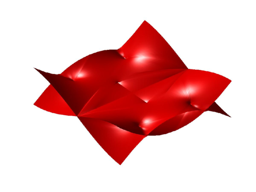
Figure 2: Branched covering of the the complex plane by the two sheet Riemann surface of the function $y=\sqrt{\left(z^{2}+a\right)\left(z^{2}+b\right)\left(z^{2}+c\right)}$. This would correspond to a main spectrum consisting of only $n=6$ points.

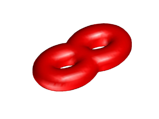
Figure 3: The hyperelliptic Riemann surface of genus $g=2$. This is topologically equivalent to the two-sheet Riemann surface shown in 2 since $n=2g+2=6$ gives $g=2$.

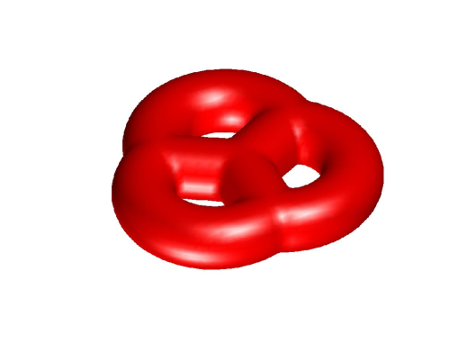
Figure 4: A hyperelliptic Riemann surface of $g=3$.

An alternative calculation of the same integral Eq.(41) is done following directly the path along the canonical cycles $a$ and $b$. In this evaluation the periodicity properties of the $\Theta$ function are essential. When the point of integration $q$ is on a $b_{k}$ cycle, the point that corresponds to it but attached to the opposite side of the cut along the cycle can be reached by a complete turn along the nearest $a$ cycle. But such a change does not introduce any modification in the integrand, since it is exactly the operation involved in the first periodicity property of $\Theta$. This means that the integration along the edge of $\Gamma$ coming from a cycle $b_{k}$ can be paired with the integration along the edge coming from the opposite side of the cut along $b_{k}$, without any change in the integrand. Since these two integrals are equal but of opposite sign we conclude that the edges originated from $b$-cycles do not contribute to the integral. Analoguous consideration for the $a_{k}$-cycles involve the second property of the $\Theta$ function. If $q$ is on an edge representing one side of the cut along the $a_{k}$ cycle, the point $\overline{q}$ on other side can be reached by a complete turn along a $b$ cycle. This introduces the change of the integrand

$$\zeta\left(q\right)\rightarrow\zeta\left(\overline{q}\right)=\exp\left\{-i\pi\tau_{kk}-2\pi i\left[\nu_{k}\left(q\right)-\phi_{k}+D_{k}\right]\right\}\zeta\left(q\right)$$

This means

$$\ln\zeta\left(\overline{q}\right) = -i\pi\tau_{kk}-2\pi i\left[\nu_{k}\left(q\right)-\phi_{k}+D_{k}\right]$$

$$+\ln\zeta\left(q\right)$$

and

$$d\ln\zeta\left(\overline{q}\right) = \frac{d\zeta\left(\overline{q}\right)}{\zeta}$$

$$= -2\pi id\nu_{k}\left(q\right)+\ln\zeta\left(q\right)$$

Taking into account the conclusion reached before that the $b$ cycles do not contribute to the integration and leaving aside the part coming from the branch cut the integral becomes

$$\frac{1}{2\pi i}\int_{\Gamma}\ln q\frac{d\zeta}{\zeta}$$

$$= \sum_{k=1}^{N}\left[\int_{a_{k}}\ln q\frac{d\zeta\left(q\right)}{\zeta}+\int_{-a_{k}}\ln\overline{q}\frac{d\zeta\left(\overline{q}\right)}{\zeta}\right]$$

$$= \sum_{k=1}^{N}\int_{a_{k}}\left\{\ln q\frac{d\zeta\left(q\right)}{\zeta}-\ln q\left[2\pi id\nu_{k}\left(q\right)+\frac{d\zeta\left(q\right)}{\zeta}\right]\right\}$$

or

$$\frac{1}{2\pi i}\int_{\Gamma}\ln q\frac{d\zeta}{\zeta}=\sum_{k=1}^{N}\int_{a_{k}}\ln qd\nu_{k}$$ (43)

This integral is a constant since $d\nu_{k}$ is a differential one-form generated from a linear combination of the canonical one-forms (depending only on the surface) and the integration is performed over closed loops $a_{k}$. It does not leave any choice since it does not depend on any parameter.

We have completed the calculation of the integral (42) in the two ways: one with the polygonal dissection of the Riemann surface plus the branch cut (which gives the right hand side of (42) ) and one with the path on the surface, using the reunion of canonical cycles, obtaining the constant of Eq.(43). It only remains to make explicit the last term in Eq.(42) coming from the branch cut integration.

$$\int_{0}^{\infty}\frac{d\zeta\left(q\right)}{\zeta}=\ln\frac{\zeta\left(\infty\right)}{\zeta\left(0\right)}$$ (44)

with the relation

$$\zeta\left(\infty\right) = \Theta\left[\mathbf{\phi+\nu}\left(\infty\right)-\mathbf{D}\right]$$

$$= \Theta\left[\mathbf{\phi+\nu}\left(0\right)+\int_{0}^{\infty}d\mathbf{\nu}\left(q\right)-\mathbf{D}\right]$$

In the argument, $\mathbf{\nu}\left(0\right)-\mathbf{D}$ is a constant that can be included in the initial phases $\phi_{k0}$ (Eq.(36)). The integrals of the differential forms are done along a path that can be completed with a circle at infinity. It results a loop can then be mapped onto the set of loops that surround the cuts, i.e. effectively it is shrinked the set of $a$-cycles. The integrals are then reduced at the diagonal entries of the $A$ matrix which are all unity.

$$\int_{0}^{\infty}d\mathbf{\nu}\left(q\right)=\frac{1}{2}\int_{C}d\mathbf{\nu}\left(q\right)=\frac{1}{2}\mathbf{I}$$

Then Eq.(44) can be written

$$\int_{0}^{\infty}\frac{d\zeta\left(q\right)}{\zeta}=\ln\left[\frac{\Theta\left(\mathbf{\phi+}\frac{1}{2}\mathbf{I}\right)}{\Theta\left(\mathbf{\phi}\right)}\right]$$

We return now to the Eq.(42) and (43)

$$\frac{1}{2\pi i}\int_{\Gamma}\ln q\frac{d\zeta}{\zeta} = \sum_{j=1}^{N}\ln\gamma_{j}-2\int_{0}^{\infty}\frac{d\zeta}{\zeta}$$

$$= \sum_{k=1}^{N}\int_{a_{k}}\ln qd\nu_{k}$$

where from we obtain

$$\sum_{j=1}^{N}\ln\gamma_{j}=2\int_{0}^{\infty}\frac{d\zeta}{\zeta}+\sum_{k=1}^{N}\int_{a_{k}}\ln qd\nu_{k}$$

The explicit form of the solution is given by the conversion formula (3.6)

$$u = 2\sum_{k=1}^{N}\ln\gamma_{k}-\sum_{m=1}^{2N}\ln p_{m}$$

$$= 4\ln\left[\frac{\Theta\left(\mathbf{\phi+}\frac{1}{2}\mathbf{I}\right)}{\Theta\left(\mathbf{\phi}\right)}\right]$$

$$+\sum_{k=1}^{N}\int_{a_{k}}\ln qd\nu_{k}-\sum_{m=1}^{2N}\ln p_{m}$$

Since the last line is composed of constants,

$$K\equiv\sum_{k=1}^{N}\int_{a_{k}}\ln qd\nu_{k}-\sum_{m=1}^{2N}\ln p_{m}$$

we can write the solution as

$$u\left(x,y\right)=4\ln\left[\frac{\Theta\left(\mathbf{\phi+}\frac{1}{2}\mathbf{I}\right)}{\Theta\left(\mathbf{\phi}\right)}\right]+K$$

with

$$\phi_{k}\left(x,y\right)=2C_{k1}\left(x-iy\right)+\phi_{k0}$$

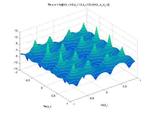
Figure 5: The solution of the Jacobs-Rebbi equation.

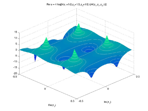
Figure 6: The solution clearly shows the vortical structures as expected.

4 Conclusion

In conclusion we have proved that the Jacobs-Rebbi equation is exactly integrable and have provided the exact solution. We have followed the standard approaches developed in detail for similar equations: sine-Gordon and sinh-Poisson equations.

Knowledge of the exact solution will make more accessible the investigation of the physical applications of this equation.

References

[1] L. Jacobs and C. Rebbi, Phys.Rev.B 19 (1976) 4486.
[2] R. Jackiw and So-Young Pi, Phys. Rev. D42, 3500
(1990).
[3] R. Jackiw and So-Young Pi, Phys. Rev. Lett. 64,
2969 (1990).
[4] G. Nardelli, Phys. Rev. D52, 5944 (1995)
[5] G. Dunne, Self-dual Chern-Simons theories,
hep-th/9410065.
[6] W. Horton and A. Hasegawa, Chaos 4 (1994) 227.
[7] R. H. Kraichnan and D. Montgomery, Rep. Prog.
Phys. 43, (1980) 547.
[8] F. Spineanu and M. Vlad, Phys.Rev.E67 (2003) 046309.
[9] M. Gregory Forest and David W. McLaughlin, J. Math. Phys
23 (1982) 1248.
[10] A.C. Ting, H.H. Chen and Y.C. Lee, Physica 26D (1987) 37.
[11] M. J. Ablowitz and H. Segur, Solitons and Inverse
Scattering Transform, SIAM, 1981.
[12] E.R. Tracy and H.H. Chen, Phys.Rev. A 37 (1988) 815.