Band gaps and localization of water waves over one-dimensional topographical bottoms

Abstract

In this paper, the phenomenon of band gaps and Anderson localization of water waves over one-dimensional periodic and random bottoms is investigated by the transfer matrix method. The results indicate that the range of localization in random bottoms can be coincident with the band gaps for the corresponding periodic bottoms. Inside the gap or localization regime, a collective behavior of water waves appears. The results are also compared with acoustic and optical situations.

When propagating through structured media, waves will be multiply reflected or scattered, leading to many interesting phenomena such as band gaps in periodic structures Mermin and localization in disordered mediaAnderson . Within a band gap, waves are evanescent; when localized, they remain confined in space until dissipated. The phenomenon of band gaps and localization has been both extensively and intensively studied for electronic, electromagnetic, and acoustic systems. A great body of literature is available, as summarized in Ref. Sheng .

The propagation of waters through underwater structures has also been widely studied, because of its importance in a number of coastal engineering problems. In particular, the consideration of band gaps has been recently applied to water wave systems Hare ; Chou ; Nature ; APL . Some of the advances have been reviewed, for example, by McIver McIver . On one hand, the most recent experiment has used water waves to demonstrate the phenomenon of Bloch waves as a result of the modulation by periodic bottom structures Nature . On the other hand, the possible band gaps have been recently proposed for water waves propagation through arrays of rigid cylinders that regularly stand in the water APL .

Relatively speaking, the more intriguing concept of Anderson localization remains less touched in the context of water waves. Although the earlier attempts do show that the localization phenomenon is possible for water waves JFM , a few important issues have not been discussed. These issues include, for example, the statistical properties of localization, the phase behavior of the localized states, single parameter scaling and universality, and the relation between localization and band gaps of corresponding periodic situations. Recent research Deych ; LY indicates that these issues are essential in discerning localization effects. As such, it might be desirable to consider the localization of water waves further.

In the present Letter, we wish to study the localization of water waves in one-dimensional randomly structured bottoms, and its relation with band gaps of the corresponding periodic bottoms. The phase behavior of the water waves in the presence of localization will also be discussed.

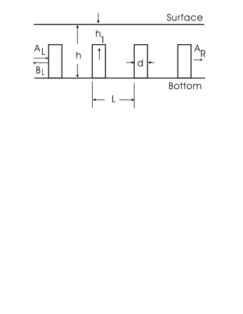
Figure 1: Conceptual layouts.

The system we consider is illustrated in Fig. 1. Here is shown that there are $N$ identical steps of width $d$ periodically placed on the bottom. The periodicity is $L$. The depth of water is $h$, and the depth of the steps is $h_{1}$. We suppose that the surface waves propagate from left to the right. The disorders are introduced as follows. The degree of disorder is measured as the percent of random displacement of the steps within a range around their original regular positions with regard to the periodic constant. Obviously the maximum (complete) randomness is $1-d/L$; half random (order) is thus $1/2-d/(2L)$.

The wavenumbers in the water ($k$) and over the steps ($k_{1}$) are determined as Ye

$$\frac{\omega^{2}}{\omega_{0}^{2}}=kL\tanh(kh),\ \mbox{and}\ \frac{\omega^{2}}{\omega_{0}^{2}}=k_{1}L\tanh(k_{1}h_{1}),$$ (1)

where $\omega_{0}=gL$. In the simulation, all lengths are scaled by $L$, and the frequency is scaled by $\omega_{0}$.

The waves on the left and right end of the step array can be expressed in the matrix form

$$\left(\begin{array}[]{c}A_{L}e^{ikx}\\ B_{L}e^{-ikx}\end{array}\right),\ \mbox{and}\ \left(\begin{array}[]{c}A_{R}e^{ikx}\\ B_{R}e^{-ikx}\end{array}\right).$$ (2)

Clearly, $A_{L}$ is the incident wave, $A_{R}$ the outgoing wave, and $B_{L}$ the reflected wave. $B_{R}$ is zero since there is no wave coming from the right. For a unit plane wave incidence, $A_{L}=1$.

By the standard transfer matrix method LY , the coefficients $A_{R},A_{L},B_{L}$ can be related by a transfer matrix. The transmission coefficient is defined as $T=\left|\frac{A_{R}}{A_{L}}\right|^{2}.$ For the periodic case, the field $\eta$ can be written in the Bloch form, $\eta(x)=e^{iKx}u(x)$, where $u(x)$ is a periodic function with the periodicity of the structure. Then the dispersion and band structure can be computed from

$$\cos(KL) = \cos(k_{1}L(d/L)\cos(kL(L-d)/L)-$$

$$\cosh(2\xi)\sin(k_{1}L(d/L))\sin(kL(L-d)/L),$$

where

$$\xi=\ln(q),\ \ \ \mbox{with}\ \ \ q^{2}=\frac{k_{1}}{k}=g_{s}^{-1}\ \ \ \Rightarrow\ \ \ \xi=-\frac{1}{2}\ln g_{s}.$$

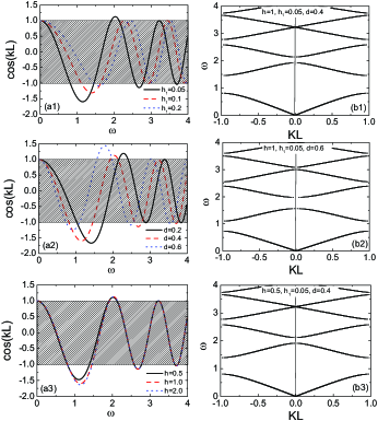
Figure 2: The dispersions and band structures versus frequency. Dispersions: (a1) Variation of the step depth with $h=1,d=0.4$; (a2) Variation of the step width $h=1,h_{1}=0.05$; (a3) Variation of the water depth with $h_{1}=0.05,d=0.04$. The variation of the band structures against $d$ and $h$: ((b1) $h=1,h_{1}=0.5,d=0.4$; (b2) $h=1,h_{1}=0.05,d=0.6$; (b3) $h=0.5,h_{1}=0.05,d=0.4$.

Fig. 2 shows the dispersion and band structures for periodic systems. Figs. 2(a1), (a2) and (a3) present the dependence of the dispersion on the variations of the depth and the width of the steps, and the water depth. The curves within or outside the dark areas refer to the passing or forbidden bands respectively. We observe the following from Fig. 2. (1) There are band gaps for water systems. But with increasing $h_{1}$, the band gaps become narrower, referring to (a1). (2) The band gaps move towards lower frequencies by increasing the width of the steps, as shown by (a2). (3) While the band structures are sensitive to the physical structures of the steps, they are rather insensitive to the variation of the water depth, as evidenced by (a3). (4) The band gaps start to disappear as the frequency increases. This is understandable. For high frequencies, especially when $kh,kh_{1}>>1$, the dispersion relation becomes $\omega^{2}=gk$, therefore the structure of the bottom has less and less effects. Some band structures are exemplified by (b1), (b2) and (b3). In our simulation, we found that the step depth $h_{1}$ is vital in determining the band structures, and subsequently the localization.

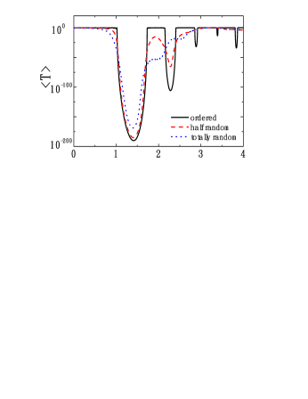
Figure 3: Transmission versus frequency for the ordered, half ordered, and completely random cases: $h=1,h_{1}=0.05,d=0.2$. Here $\langle\cdot\rangle$ refers to the average over the random configurations, and totally 100 steps are consideration in the computation.

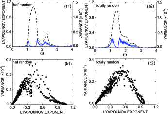
Figure 4: The behavior of the Lyapunov exponent and its variance. Here $h=1,h_{1}=0.05,d=0.2.$

In Fig. 3, we show the transmission versus frequency for different randomness. As a comparison, the transmission for the ordered case is also shown. The results indicate the following. (1) There are well defined inhibited transmission ranges for the ordered case, coincident with the band gaps shown in Fig. 2. And these ranges decrease with frequency, until disappear. The degree of inhibition more or less decreases with frequency. These features differ from those in optical and acoustic systems LY ; Maradudin . (2) The disorder tends to reduce the transmission for the mid range of frequency, but it has less influences for low or high frequencies, implying that the scattering by the steps is weak in these ranges. The inhibition in the presence of disorders is an indication and measure of localization. (3) Within the band gaps, the disorder tends to enhance the wave propagation, a feature that has been also discovered previously in the optical and acoustic systems LY ; Maradudin . But different from these systems, the inhibition starts to decease as frequency increases. We also notice that in some cases the strong localization is coincident with the band gaps, particularly for the first two band gaps. (4) The level of localization does not necessarily depend on the degree of disorders. For example, within the first band gap, the wave is more localized for the half random than the completely random case.

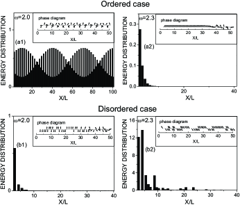
Figure 5: Energy distribution and the phase behavior (insets) for the ordered and totally random cases. The structure parameters are the same as in Fig. 4.

We have also studied the statistical properties of localization by considering the Lyapounov exponent (LE) $\gamma=\lim_{N\rightarrow\infty}\langle-\frac{1}{N}\ln(T)\rangle$, where $N$ is the number of steps, and its variance as a function of frequency. LE characterizes the degree of localization, and its variance signifies the transition behavior. The results are shown in Fig. 4. The parameters are indicated in the caption. Here we see that behavior of LE mimics the hand structures, particularly for weak disorders. Similar to the optical case Deych , but contrary to the acoustic case LY , there are two double maxima for the variance inside the gaps. This feature is more prominent in the low frequency bands. Different from both optical and acoustic cases, the double peak feature in the variance does not disappear even in the complete random case, depicted by (a2). We also plot LE versus its variance in Fig. 4. Here even in the totally random situation, we do not observe the linear dependence between LE and its variance in contrast to the expectation from the scaling analysis of localization SST .

The energy distribution and the phase behavior of water waves in the ordered and disordered cases are shown in Fig. 5. The energy is defined as the modulus of the waves, and the phase $\theta$ is defined from $\eta=|\eta|e^{i\theta}$. To show the phase behavior, we associate a phase vector to the phase as $\vec{v}=(\cos\theta,\sin\theta)$ and the phase vector is plotted in two-dimensions. Two frequencies are chosen to be inside and outside the second gap, referring to Fig. 3. Comparing the ordered and disordered cases, we observe clearly that the energy or the wave is indeed confined by the disorder to the site of transmission. But the decay of the energy along the path does not follow the exponential feature. Here we see, within the gaps in the ordered case or when the localization occurs, the phase vectors at different space points tends to point to the same or the opposite directions. Such a collective behavior of water waves has not been discussed before. At the end of the step arrays, there is some disorientation in the pointing directions of the phase vectors. This is due to the finite size effect.

In summary, we have applied the concept of band gaps and localization to water surface waves in a one-dimensional system. The statistical properties of localization and their relation with corresponding band gaps are studied. It is shown that localization is related to a coherent behavior of the system.

Acknowledgements The work received support from Natural Science Foundation of China (No.10204005), and the Shanghai Bai Yu Lan fund (ZY).

References

- (1) N. W. Ascroft and N. D. Mermin, Solid State Physics (Saunders College, Philadelphia, 1976).
- (2) P. W. Anderson, Phys. Rev. 109, 1492 (1958).
- (3) P. Sheng, Introduction to Wave Scattering, Localization, and Mesoscopic Phenomena (Academic Press, New York, 1995).
- (4) T. J. O’Hare and A. G. Davies, Appl. Ocean Res. 15, 1 (1993).
- (5) T. Chou, Phys. Rev. Lett. 79, 4802 (1997).
- (6) M. Torres, J. P. Adrados, F. R. Montero de Espinosa, Nature 398, 114 (1999).
- (7) Y.-K. Ha, J.-E. Kim, H.-Y. Partk, and I.-W. Lee, Appl. Phys. Lett. 81, 1341 (2002).
- (8) P. McIver, Appl. Ocean Res. 24, 121 (2002).
- (9) P. Devillard, F. Dunlop, and B. Souillard, J. Fluid Mech. 186, 521 (1988); M. Belzones, E. Guazzelli, and O. Parodi, J. Fluid Mech. 186, 539 (1988).
- (10) L. I. Deych, A. A. Lisyansky, and B. L. Altshuler, Phys. Rev. Lett. 84, 2678 (2000).
- (11) Pi-Gang Luan and Zhen Ye, Phys. Rev. E 63, 066611 (2001).
- (12) Z. Ye, Phys. Rev. E 67, 036623 (2003).
- (13) A. R. McGurn, K. T. Christensen, F. M. Mueller, and A. A. Maradudin, Phys. Rev. B 47, 13120 (1993)
- (14) E. Abrahams, P. W. Anderson, D. C. Licciardello, and T. V. Ramakrishnan, Phys. Rev. Lett. 42, 673 (1979).