Focusing a radially polarized light beam to a significantly smaller spot size

Abstract

We experimentally demonstrate for the first time that a radially polarized field can be focussed to a spot size significantly smaller (0.16(1)$\lambda^{2}$) than for linear polarization (0.26$\lambda^{2}$). The effect of the vector properties of light is shown by a comparison of the focal intensity distribution for radially and azimuthally polarized input fields. For strong focusing a radially polarized field leads to a longitudinal electric field component at the focus which is sharp and centered at the optical axis. The relative contribution of this component is enhanced by using an annular aperture.

A large number of optical instruments and devices make use of a sharply focussed light beam. Prominent examples are in lithography, confocal microscopy, optical data storage as well as in particle trapping. A highly concentrated and well matched field is also a necessary requirement for manipulating nanoscopic quantum systems in quantum information processing or cavity quantum electrodynamics KimbleEnk . When reaching for the limits the polarization properties of the electromagnetic field play a dominant role. For a vectorial description of strong focusing using high numerical apertures different methods have been developed RichardsWolf ; MansuripurJOSAA ; KantJModOpt ; SheppardMultipoleJModOpt . It turns out that in general all three mutually orthogonal field components appear at the focal region. The electric energy density patterns of individual polarization components were mapped using single molecules with the absorption dipole axis pointing in the three different directions HechtJMicroscopy ; NovotnyYoungworthPRL ; HechtNovotnyPRL . For linearly polarized light, the energy density distribution of a longitudinally polarized component in the direction of propagation of the beam is not rotationally symmetric. This primarily causes an asymmetric deformation of the focal spot. When using an annular aperture, the relative contribution of the longitudinal component is increased and the asymmetry becomes more pronounced SheppardAnnularApert . These asymmetries were recently confirmed experimentally DornJModOptics . In addition, it was predicted that a special polarization pattern is needed for focusing down to the smallest possible spot QuabisOptComm .

The effects of the vector properties of light on the structure of the focus are best observed if one compares two special input beams with identical intensity distribution but different polarization properties. A good example for two such fields are an azimuthally and a radially polarized field with identical doughnut shaped intensity distributions. When focusing with a high numerical aperture the radially polarized input field leads to a strong longitudinal electric field component in the vicinity of the focus ScullyZubairyPRA ; QuabisOptComm . In contrast, the azimuthally polarized field generates a strong magnetic field on the optical axis NovotnyQuantumDotSpectroscopy while the electric field is purely transverse and zero at centre YoungworthOpticsExpress . In general, the direction of the polarization may vary largely inside the focal spot. Especially when sub–wavelength–structures are investigated this has to be carefully considered in a quantitative analysis WilsonOptComm . The predicted axial light forces acting on particles in an optical tweezer set up are different in a vectorial treatment as compared to theories based on paraxial and geometric optics NussenzveigOptPinzette . The specific interaction of the different field components at the focus with single molecules can provide information about the orientation of the absorption dipole of the molecules HechtJMicroscopy ; NovotnyYoungworthPRL . Although these field components may also occur in the vicinity of near field apertures BetzigScience , a far field technique can be advantageous as it avoids a modification of the dynamics of the molecule due to an interaction with the probe XieDunnScience ; AmbroseScience . For the spectroscopy of magnetic dipole transitions in quantum dots it was proposed to use an azimuthally polarized field for the excitation and take advantage of the strong magnetic and the vanishing electric field component on axis NovotnyQuantumDotSpectroscopy . To couple efficiently to small quantum systems such as single atoms the incoming field must be well matched in both its amplitude and phase but also in its polarization properties KimbleEnk .

The vector properties not only affect the local field direction but also the intensity distribution at the focus. This is experimentally demonstrated here below by comparing highly resolved measurements for azimuthally and radially polarized input fields. The radially polarized beam can have a narrow central peak due to the appearance of the strong longitudinal field component that is sharply centered around the optical axis. The experimental results reported here confirm for the first time, to the best of our knowledge, that a radially polarized input field leads to the smallest possible spot size in far field focusing observed so far. Three different types of set up have been described with which a radially or azimuthally polarized doughnut mode can be produced . Most of them either generate the mode inside a laser resonator Pohl ; Niziev or use a Mach–Zehnder like interferometer Tidwell ; YoungworthSPIE . A third approach involves the use of mode–forming holographic and birefringent elements Tschudi .

Figure 1: Experimental set up to measure the focal intensity distribution. MO: Leica plan–apo 100x, 0.9, OD: optical diode, HWP: half–wave plate, TL: telescope lenses, PH: pinhole, PC: polarization converter, FL: focusing lens, NCFPI: non–confocal Fabry–Perot interferometer, CL: collimating lens, AS: aperture stop, M: four mirrors for polarization insensitive deflection (details not shown), MD: monitor diode, PD: photo diode partially covered with gold–zinc alloy

Here we use another approach for the generation of this polarization mode. The TEM₀₀–beam of a linearly polarized, single mode helium–neon laser ($\lambda$=632.8nm) is expanded and collimated by a telescope with an additional pinhole as a mode cleaner (Fig. 1). The collimated beam is then sent through a polarization converter. This element consists of four half–wave plates, one in each quadrant. The optical axis of each segment is oriented such that the field is rotated to point in the radial direction. However, due to the limited number of segments and some diffraction losses at the boundaries between adjacent segments, the field is not perfectly radially polarized. Nevertheless, this field has a large overlapp with the desired mode and a smaller overlapp with additional higher order transverse modes. These undesired modes are filtered out by sending the beam through a non– confocal Fabry–Perot interferometer that is operated as a mode–cleaner and which is kept resonant only for the radially or azimuthally polarized doughnut–mode. With this method, a purity of $>$99% is achieved.

The beam was collimated such that the beam radius at the maximum intensity was 1.2mm. To ensure minimum wave front aberrations we analyzed the beam with a Shack–Hartmann wave front sensor yielding a root mean square wave front error $<\lambda/35$. By rotating the polarization of the beam before the polarization converter by 90^∘, it is possible to switch between a radially and an azimuthally polarized beam. For measurements with an annular aperture, a stop is placed directly in front of the microscope objective to block the inner part of the beam. The stop is a high quality glass substrate (surface accuracy of $<\lambda/20$) coated with an opaque disc (d_i=3.0mm or 3.3mm). The diameter of the entrance pupil of the focusing microscope objective (NA=0.9) is 3.6mm. To measure the focal intensity distribution we used an experimental set up which is based on the knife edge method. The edge is formed by a sharp edged opaque pad that is deposited on the active surface of a photodiode. Therefore no subsequent optical system is needed to collect the transmitted light and effects due to diffraction at the edge are minimized. A more detailed description of the properties of the sensor is given in DornJModOptics . The knife edge method allows one to measure the one dimensional projection i.e. the line integrated intensity of the two dimensional intensity distribution onto the direction along which the edge is moved. By measuring a set of projections onto different directions one acquires the input data needed for a tomographic reconstruction of the two dimensional intensity distribution, using e.g. the Radon back–transformation formalism ImageReconstruction .

For rotationally symmetric input fields the focal spot also shows rotational symmetry and all projections onto any line are identical. Therefore one representative measurement would in principle suffice. But we measured projections onto two orthogonal lines to exclude the possibility that the symmetry of the focussed field is affected by non–spherical aberrations introduced e.g. by the microscope objective. The results were identical within the limits of reproducibility. Line integrals of the intensity distribution were also measured for different positions of the knife edge sensor with respect to the focal plane. This yields a line integrated cross section of the propagating beam containing the optical axis (Fig. 2).

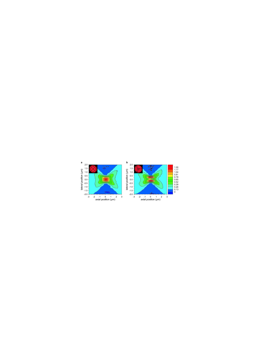
Figure 2: Defocus series for a radially (a) and azimuthally (b) polarized input field. The insets illustrate how the polarization of the input beam varies spatially across the beam cross section. Note that identical initial intensity distributions lead to different distributions at focus.

An evidence for the strong longitudinal electric field at the focus of the radially polarized beam is the fact that the intensity projection shows a maximum on the optical axis in the focal plane (Fig. 2a). In contrast, the azimuthally polarized beam has no longitudinal field component and on the optical axis the intensity projection has a minimum. The measured projections in the focal plane are shown in figure 3 for the two modes along with the calculated distributions of the transverse and longitudinal field components. The curves were normalized such that for each case the total intensity in the focal spot equals 1 (arbitrary unit). Cross sections for the tomographically reconstructed intensity distributions (Fig. 3) show that the intensity on the optical axis vanishes for the azimuthally polarized beam. The beam profile at the focus is very similar to the doughnut shaped profile of the input beam just as one would naively expect based on the scalar diffraction theory.

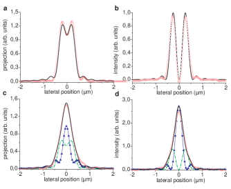
Figure 3: Measured projections (a,c) and cross sections through the tomographically reconstructed intensity distributions (b,d) in the focal plane for an azimuthally (a,b) and a radially (c,d) polarized input field. Open squares: experimental data; calculated curves: solid black line: total field; dashed line: transverse field; solid triangles: longitudinal field

In contrast, the radially polarized mode leads to a narrow peak around the optical axis where the field is basically directed into a longitudinal direction. The transverse field components show a profile very similar to the profile of the azimuthally polarized beam. The power contained in the longitudinal field is calculated to be 49.6% of the total beam power. The relative contribution of the longitudinal component can be enhanced when the numerical aperture of the focusing system is increased.
For a numerical aperture of 0.9 as in this experiment the calculated spot size associated with this longitudinal field alone is 0.2$\lambda^{2}$ which is below the spot size for a linearly polarized input field with homogeneous intensity distribution (0.31$\lambda^{2}$). The spot size of the total field is still larger (0.47$\lambda^{2}$) than for linear polarization due to the broad distribution of the additional transverse field component. We note in passing that, in general, a calculation using a scalar field tends to underestimate the spot size for large numerical apertures. The reason is that due to the vector properties of light the plane waves that form the focussed field in image space cannot interfere perfectly at the focus as the electric (and magnetic) field vectors are not all parallel at the focus.

In the case of the radially polarized doughnut mode the rays that propagate under a small angle to the optical axis show only a small longitudinal component. The stronger transverse field components associated with these waves all cancel out on the optical axis and form a broad, doughnut shaped profile which increases the spot size. But when an annular aperture is used for focusing, only waves that propagate under a large angle to the optical axis contribute to the focal field. For a high numerical aperture and a large inner radius of the annular aperture the electric field vectors for a radially polarized

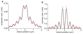
Figure 4: Projection of (a) and cross section through (b) the tomographically reconstructed intensity distribution for an azimuthally polarized input field focussed using an annular aperture (d_i=3.0mm). Open squares: experimental data; solid black line: calculated curve for the total field

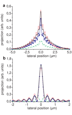
Figure 5: Measured projection of (a) and cross section through (b) the tomographically reconstructed intensity distribution for a radially polarized input field focussed using an annular aperture (d_i=3.3mm). The calculated power contained in the longitudinal field amounts to 72.8% of the total beam power. Open squares: experimental data; calculated curves: solid black line: total field; dashed line: transverse field; solid triangles: longitudinal field

input field are essentially parallel to the optical axis. All rays interfere perfectly and consequently the spot size is close to the spot size which one would calculate using a scalar theory. Cross sections through the tomographically reconstructed intensity distributions are shown for an azimuthally (Fig. 4) and for a radially (Fig. 5) polarized input field when using the annular aperture. Compared to the case without annular aperture the sidelobes are more pronounced in both cases, indicating that the relative contribution of the intensity in the side lobes has increased at the expense of a decreased central maximum.

The spot size for radial polarization with annular aperture is reduced to 0.16(1)$\lambda^{2}$ (theoretical value 0.17$\lambda^{2}$) (Fig. 5b). This is well below 0.26$\lambda^{2}$, the theoretically achievable spot size for linear polarization under the same experimental conditions and also well below 0.22$\lambda^{2}$, the theoretical value for circularly polarized light. The latter is a little smaller as compared to linear polarization due to the definition of the spot size used here.

Expressed in units of $\lambda^{2}$ this is to our knowledge the smallest measured spot size that has been reached in far field focusing in air (NA$<$1).

It is worth noting that for a radially polarized input field, the magnetic field vectors point in the azimuthal direction just as the electric field vectors do for an azimuthally polarized input beam. The magnetic energy density distribution for a radially polarized beam shows the same distribution as the electric energy density distribution for an azimuthally polarized beam and vice versa.

In summary, we have experimentally verified the influence of the polarization on the shape of the focal spot. For a radially polarized field distribution with annular aperture, the focal spot size was reduced to the smallest focal spot observed up to now when normalizing to the wavelength ($\lambda^{2}$). The experimentally observed spot size for NA=0.9 is about 35% below the theoretical limit for linearly polarized light. The calculated spot size for the longitudinal field alone is 0.14$\lambda^{2}$. Therefore, if a surface is covered with a special photosensitive layer which is only sensitive to the narrow longitudinal field distribution QuabisOptComm even smaller spot sizes can be reached. These ideas may well be combined with other concepts for the increase of transverse resolution such as the solid immersion lens KinoSIL or coupling to small mesoscopic antennae BouhelierEtAlPRL . A radially polarized field will also provide the input field which is best suited for coupling into the recently proposed all–dielectric waveguide IbanescuScience .

- (1) S. J. van Enk, and H. J. Kimble, Phys. Rev. A 63, 023809 (2001)
- (2) B. Richards and E. Wolf, Proc. R. Soc. London A 253, 358 (1959)
- (3) M. Mansuripur, J. Opt. Soc. Am. A 3, 2086 (1986) and 10, 382 (1993)
- (4) R. Kant, J. Mod. Opt. 40, 337 (1993)
- (5) C. J. R. Sheppard, and P. Török, J. Mod. Opt. 44, 803 (1997)
- (6) B. Sick, B. Hecht, U. P. Wild, and L. Novotny, J. of Microsc. 202, 365 (2001)
- (7) L. Novotny, M. R. Beversluis, K. S. Youngworth, and T. G. Brown, Phys. Rev. Lett. 86, 5251 (2001)
- (8) B. Sick, B. Hecht, and L. Novotny, Phys. Rev. Lett. 85, 4482 (2000)
- (9) C. J. R. Sheppard, J. Opt. Soc. Am. A 18, 1579 (2001)
- (10) R. Dorn, S. Quabis, and G. Leuchs, J. Mod. Opt. 50, 1917 (2003); arxiv/physics/030401
- (11) S. Quabis et al., Opt. Comm. 179, 1 (2000)
- (12) M. O. Scully, and M. S. Zubairy, Phys. Rev. A 44, 2656 (1991)
- (13) J. R. Zurita–Sánchez, and L. Novotny, J. Opt. Soc. Am. B 19, 2722 (2002)
- (14) K. S. Youngworth, and T. G. Brown, Optics Express 7, 77 (2000)
- (15) T. Wilson, J. Juškaitis, and P. Higdon, Opt. Comm. 141, 298 (1997)
- (16) P. A. Maia Neta, and H. M. Nussenzveig, Europhys. Lett. 50, 702 (2000)
- (17) E. Betzig, and R. J. Chichester, Science 262, 1422 (1993)
- (18) X. S. Xie, and R. C. Dunn, Science 265, 361 (1994)
- (19) W. P. Ambrose, P. M. Goodwin, J. C. Martin, and R. A. Keller, Science 265, 364 (1994)
- (20) D. Pohl, Appl. Phys. Lett. 20, 266, (1972)
- (21) A. V. Nesterov, V. G. Niziev, and V. P. Yakunin, J. Phys. D: Appl. Phys. 32, 2871 (1999)
- (22) S. C. Tidwell, D. H. Ford, and W. D. Kimura, Appl. Opt. 29, 2234 (1990)
- (23) K. S. Youngworth, and T. G. Brown, Proc. SPIE 3919 (2000)
- (24) E. G. Churin, J. Hoßfeld, and T. Tschudi, Opt. Comm. 99, 13 (1993)
- (25) S. W. Rowland, Computer Implementation of Image Reconstruction Formulas. In ”Image Reconstruction from Projections”, pp. 9-78, edited by G. T. Herman (Springer, Berlin, 1979)
- (26) I. Ichimura, S. Hayashi, and G. S. Kino, Appl. Opt. 36, 4339 (1997)
- (27) A. Bouhelier, M. Beversluis, A. Hartschuh, and L. Novotny, Phys. Rev. Lett. 90, 013903 (2003)
- (28) M. Ibanescu et al., Science 289, 415 (2000)