Near-field diffraction of fs and sub-fs pulses: super-resolutions of NSOM in space and time

Abstract

The near-field diffraction of fs and sub-fs light pulses by nm-size slit-type apertures and its implication for near-field scanning optical microscopy (NSOM) is analyzed. The amplitude distributions of the diffracted wave-packets having the central wavelengths in the visible spectral region are found by using the Neerhoff and Mur coupled integral equations, which are solved numerically for each Fourier’s component of the wave-packet. In the case of fs pulses, the duration and transverse dimensions of the diffracted pulse remain practically the same as that of the input pulse. This demonstrates feasibility of the NSOM in which a fs pulse is used to provide the fs temporal resolution together with nm-scale spatial resolution. In the sub-fs domain, the Fourier spectrum of the transmitted pulse experiences a considerable narrowing that leads to the increase of the pulse duration in a few times. This imposes a limit on the simultaneous resolutions in time and space.

I Introduction

The near-field diffraction of light by sub-wavelength apertures and its implication for near-field scanning optical microscopy (NSOM) has been investigated over the last decade Poh ; Nie . In NSOM, a sub-wavelength aperture illuminated by a continuous wave is used as a near-field light source providing the super (sub-wavelength) resolution in space. In the last few years, a big interest of researchers attracted the study of near-field diffraction of ultra-short light pulses aimed at obtaining the simultaneous super-resolutions in space and time (for example, see the studies Lew ; Betz ; Xie ; Amb ; Nah ; Bro ; Mit1 ; Mit2 ; Kuk1 and references therein). The studies of NSOM-pulse system primarily dealt with the diffraction of relatively long (ps) far-infrared pulses by $\mu$m-size apertures Nah ; Bro ; Mit1 ; Mit2 . It was shown that at particular experimental conditions a ps pulse experiences significant spectral Mit1 ; Mit2 and temporal Nah ; Bro ; Mit1 ; Mit2 deformations when diffracted by a $\mu$m-size aperture. The deformations lead to a modification of the temporal resolution associated with the incident ps-pulse. The recent study Mit1 indicated that spatial resolution of the NSOM performing with ps pulses is defined by the aperture size and it is independent of the wavelength.

The use of ps pulses in NSOM provides ps temporal resolution together with $\mu$m-scale spatial resolution. The achievement of higher simultaneous resolutions in space and time is challenging. The NSOM performing with a continuous wave provides nm-scale spatial resolution Poh ; Nie . High-harmonic generation produces near 0.5-fs (500 as) wave-packets with  50-nm central wavelengths Pau ; Hen . A method of generation of sub-as pulses has been already suggested in Ref. Kap . The perspective is the achievement of the simultaneous nm-scale spatial resolution together with the fs or sub-fs temporal resolution. In the visible spectral region, which is the most important domain for potential applications, the NSOM-pulse system can be realized using the conventional setup of NSOM. Unfortunately, the capabilities and limits of simultaneous spatial and temporal resolutions of such a system are not known. From a theoretical point of view, the most important questions are the degree of collimating, the duration of the ultra-short pulse past the sub-wavelength aperture and the rate of spatial and temporal broadening of the pulse farther from the aperture. To address these questions, the near-field diffraction of fs and sub-fs pulses by a nm-size slit-type aperture in a perfectly conducting thick screen is theoretically studied in the present paper.

The article is organized as follows. The theoretical approach used for finding the amplitude distribution of the ultra-short pulse in the near-field diffraction zone of the sub-wavelength aperture is described in Section II. Results of computer simulation of the near-field diffraction and discussion of the capabilities and limits of simultaneous spatial and temporal resolutions of the NSOM-pulse system are presented in Section III.

II Theory

Owing to the complicity of boundary conditions of the near-field diffraction experiment, the solution of the Helmholtz wave-equation even for a continuous wave can be obtained only by extremely extended computations. In order to simplify the computations, the NSOM model is usually restricted to two dimensions of a slit-type aperture Nee ; Bet . The combination of NSOM with an ultra-short pulse makes the numerical analysis of the problem even more difficult. In the present article, we consider a model of the NSOM-pulse system based on the transmission of fs and sub-fs pulses through a nm-size slit-type aperture in a perfectly conducting thick screen. The amplitude distribution of the diffracted wave-packet is found by using the Neerhoff and Mur coupled integral equations Nee ; Bet , which are solved numerically for each Fourier’s component of the wave-packet.

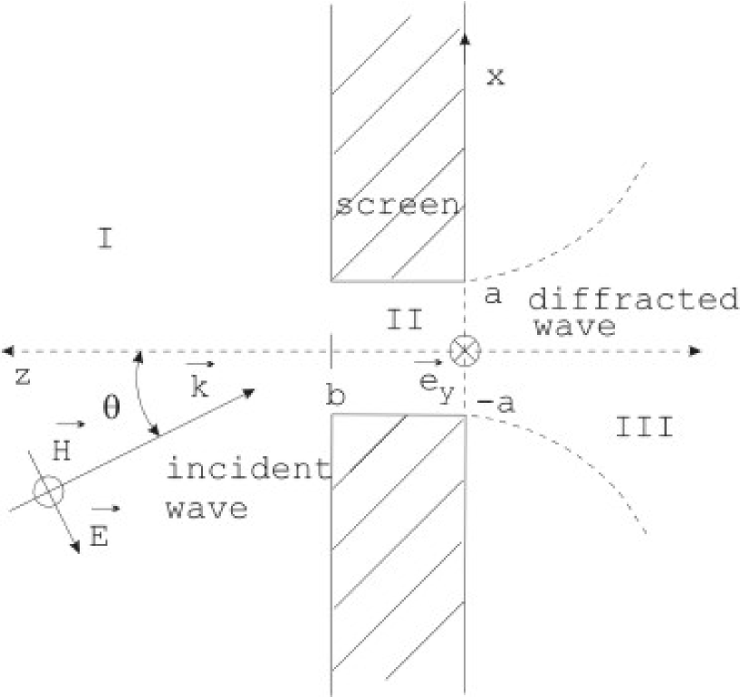
Figure 1: Schematic diagram of NSOM.

Let us briefly describe the integral approach of Neerhoff and Mur, which was developed in the studies Nee ; Bet for finding the near-field distributions of the amplitude and intensity of a continuous wave diffracted by a sub-wavelength slit in a perfectly conducting thick screen. In the region I, the continuous plane wave falls onto the slit at an angle $\theta$ with respect to the $z$-axis in the $x-z$ plane, as shown in Fig. 1. The slit width and the screen thickness are $2a$ and $b$, respectively. The magnetic field of the incident wave is assumed to be time harmonic and both polarized and constant in the direction $y$:

$${\vec{H}}(x,y,z,t)=U(x,z){\exp}(-i\omega{t}){\vec{e}}_{y}.$$ (1)

The electric field of the incident wave is found by using the Maxwell equations for the field ${\vec{H}}$. The restrictions in Eq. 1 reduce the diffraction problem to one involving a single scalar field in only two dimensions. The Green function approach Nee ; Bet uses the multipole expansion of the field with the Hankel functions in the regions I and III and with the waveguide eigenmodes in the region II. The expansion coefficients are determined by using the standard boundary conditions for a perfectly conducting screen. In region III, the near-field distributions of the magnetic ${\vec{H}}(x,z,t)$ and electric ${\vec{E}}=E_{x}{\vec{e}}_{x}+E_{y}{\vec{e}}_{y}$ fields of the diffracted wave are given by

$${\vec{H}}(x,z,t)=i{\frac{a}{N}}{\frac{\epsilon_{3}}{\epsilon_{2}}}{\sum_{j=1}^{N}}H_{0}^{(1)}[k_{3}((x-x_{j})^{2}+z^{2})^{1/2}](D{\vec{U}}_{0})_{j}{\exp}(-i\omega{t}){\vec{e}}_{y},$$ (2)

$$E_{x}(x,z,t)=-{\frac{a}{N}}{\frac{\sqrt{\epsilon_{3}}}{\epsilon_{2}}}{\sum_{j=1}^{N}}{\frac{z}{((x-x_{j})^{2}+z^{2})^{1/2}}}H_{1}^{(1)}[k_{3}((x-x_{j})^{2}+z^{2})^{1/2}](D{\vec{U}}_{0})_{j}{\exp}(-i\omega{t}),$$ (3)

$$E_{z}(x,z,t)=-{\frac{a}{N}}{\frac{\sqrt{\epsilon_{3}}}{\epsilon_{2}}}{\sum_{j=1}^{N}}{\frac{x-x_{j}}{((x-x_{j})^{2}+z^{2})^{1/2}}}H_{1}^{(1)}[k_{3}((x-x_{j})^{2}+z^{2})^{1/2}](D{\vec{U}}_{0})_{j}{\exp}(-i\omega{t}),$$ (4)

where $\epsilon_{i}$ and $k_{i}$ are respectively the permittivity and the wave number in the regions $i$ = I, II and III; $x_{j}=2a(j-1/2)/N-a$, with $j=1,2,...,N$ and $N>2a/z$; $H_{0}^{(1)}$ and $H_{1}^{(1)}$ are the Hankel functions. The coefficients $(D{\vec{U}}_{0})_{j}$ are computed by solving a set of the Neerhoff and Mur coupled integral equations Bet . For more details of the integral approach of Neerhoff and Mur see Refs. Nee ; Bet .

We now consider the near-field diffraction of an ultra-short light pulse. For the sake of simplicity, we assume that a pulse falls normally ($\Theta=0$) on the aperture. The magnetic field of the incident pulse is assumed to be Gaussian-shaped in time and both polarized and constant in the direction $y$:

$${\vec{H}}(x,y,z,t)=U(x,z){\exp[-2\ln(2)(t/{\tau})^{2}]}{\exp}(-i\omega_{0}{t}){\vec{e}}_{y},$$ (5)

where $\tau$ is the pulse duration and $\omega_{0}$ is the central frequency. The pulse can be composed in the wave-packet form of a Fourier time expansion Kuk2 :

$${\vec{H}}(x,y,z,t)=\int_{-{\infty}}^{{\infty}}{\vec{H}}(x,z,\omega){\exp}(-i\omega{t})d\omega.$$ (6)

The field distribution of the diffracted pulse is found by using the expressions (2-4) for each Fourier’s $\omega$-component of the wave-packet (6). The algorithm was implemented numerically in section III. In the computations, we used the discrete Fast Fourier Transform (FFT) of the function ${\vec{H}}(x,y,z,t)$ instead of the integral composition (6). The spectral interval $[\omega_{min},\omega_{max}]$ and the sampling points $\omega_{i}$ were optimized by matching the FFT composition to the original function (5).

III Results and discussion

In this section, the amplitude distribution of the diffracted pulse is found by using the expressions (2-4) for each Fourier’s $\omega$-component of the wave-packet (6). In order to establish guidelines for the computational results, we first consider the dependence of the amplitude of a time-harmonic continuous plane wave (a FFT $\omega$-component of the wave-packet) transmitted through the aperture on the the wave frequency $\omega=2{\pi}c/{\lambda}$. The amplitude of a transmitted FFT $\omega$-component depends on the frequency $\omega$. Owing to this effect, the Fourier spectra and duration of the wave-packet are changed under propagation through the aperture leading to modification of the temporal and spatial resolutions associated with the input pulse. The dispersion for a time-harmonic continuous wave is usually described by the normalized transmission coefficient $T_{cw}$. The coefficient is calculated by integrating the normalized energy flux $S_{z}/S_{z}^{i}$ over the slit value Bet ; Har :

$$T_{cw}=-\frac{\sqrt{\epsilon_{1}}}{4a\cos{\theta}}\int_{-a}^{a}{\lim_{z\rightarrow{0^{-}}}}[(E_{x}H_{y}^{*}+E_{x}^{*}H_{y})]dx,$$ (7)

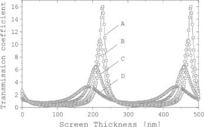
Figure 2: Transmission coefficients for a continuous wave having $\lambda=500$nm as a function of screen thickness $b$ for the different aperture widths $2a$: $A$ - 10 nm, $B$ - 15 nm, $C$ - 25 nm and $D$ - 50 nm.

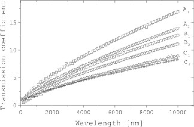
Figure 3: The dependence $T_{cw}=T_{cw}(\lambda)$ for the given values of $a$ and $b$. For $b=0$, the values $2a$: $A_{1}$ - 10 nm, $B_{1}$ - 15 nm and $C_{1}$ - 25 nm. For $b=5$nm, the values $2a$: $A_{2}$ - 10 nm, $B_{2}$ - 15 nm and $C_{2}$ - 25 nm.

where $S_{z}^{i}$ is the energy fluxe of the the incident wave of unit amplitude; $S_{z}$ is the transmitted flux. The first objective of our computer analysis was to check the consistency of the results by comparing the transmission coefficients calculated in the studies Bet ; Har with those obtained by our computations. We have computed the coefficient $T_{cw}=T_{cw}(\lambda,a,b)$ for different slit widths $2a$ and a variety of screen thicknesses b. The results are presented in Fig. 2 for the wavelength $\lambda$=500 nm. We notice that the transmission resonances of $\lambda/2$ periodicity Bet ; Har are reproduced. Furthermore, the resonance positions and the peak heights ($T_{cw}{\approx}{\lambda}/{2\pi}a$ Bet , at the resonances) are in agreement with the results Bet ; Har . Notice, that $T_{cw}{\approx}{\lambda}/{2\pi}a>1$ in the case of $a<{\lambda}/{2\pi}$. The dispersion $T_{cw}=T_{cw}(\lambda)$ for the given values of $a$ and $b$ is shown in Fig. 3. We notice that the the amplitude of the short-wavelength waves is practically unchanged, while the amplitude of the long-wavelength components increases. Thus, effectively, the aperture ”cuts off” the short-wavelength FFT-components of the wave packet (6).

Owing to the ”cut-off frequency” effect, the Fourier spectrum of the wave-packet narrows under transmission through the aperture. According to the Fourier analysis, the decrease of the spectral width of the wave packet leads to increase of the pulse duration and to modification of the temporal resolution associated with the incident pulse. The capabilities and limits of simultaneous spatial and temporal resolutions of the NSOM-pulse system are not known. From a theoretical point of view, the most important questions are the degree of collimating, the duration of the ultra-short pulse past the sub-wavelength aperture and the rate of spatial and temporal broadening of the pulse farther from the aperture. To address these questions, the near-field amplitude distributions of fs and sub-fs pulses passed through a nm-size slit-type aperture was computed. The amplitude distribution $|{\vec{E_{x}}}|$ of the diffracted wave-packet was computed for different values of the incident-pulse duration $\tau$, central wavelength $\lambda_{0}=2{\pi}c/\omega_{0}$, slit width $2a$ and screen sickness $2b$. As an example, the distribution $|{\vec{E_{x}}}|$ is shown at the three distances $z$ from the screen: at the edge of the screen $(z=-0.1a)$, in the near-field $(z=-a)$ and far-field $(z=-10a)$ zones of the diffraction (Figs. 4 and 5). Figures 4 and 5 show the amplitude distributions for the cases of $\tau$ = 2 fs and 750 as, respectively. Notice, that the value $2a=50$ nm is the minimum aperture size, which is generally accepted for the practical near-field ($z\approx{-a}$) microscopy in the visible spectral region ($\lambda\approx{500}$nm) Bet .

Analysis of Figs. 4(a) and 5(a) shows that the pulse is collimated to exactly the aperture width at the edge of the screen. Hence, the basic concept of NSOM remains valid for the ultra-short pulses: the fs or sub-fs pulse passing through a nm-size aperture can be used to provide a sub-wavelength (nm-scale) image, super-resolution in space. We notice that in the case of Fig. 4a, the duration ${\tau}^{\prime}$ of the diffracted pulse at the screen edge is practically the same as that of the incident pulse (${\tau}^{\prime}\approx{2}$fs). Thus, the temporal resolution associated with the duration of the incident 2-fs pulse is practically unchanged past the aperture. This demonstrates the possibility of the simultaneous nm-scale resolution in space and the fs resolution in time. In the case of the attosecond pulse ($\tau=750$as), the Fourier spectrum of the transmitted pulse experiences sufficient narrowing. This leads to the increase of the pulse duration in a few times (Fig. 5(a)). In the visible spectral region, this effect imposes a limit on the simultaneous spatial and temporal resolutions. It could be noted that the increase of the pulse duration in the case of the attosecond pulses can be reduced by decreasing of the central wavelength of the incident wave-packet Kuk1 . Further analysis of Figs. 4(a) and 5(a) indicates that the amplitude distribution of the diffracted wave-packet is characterized by the formation of maxima at the rims of the aperture. Notice, that the similar effect exists in the case of the near-field diffraction of a continuous wave Nov .

The results presented in Figs. 4(b) and 5(b) indicate the possibilities and limits of the simultaneous spatial and temporal resolutions at the distance $(z=-a)$. In the case of the 2-fs incident pulse, the spatial resolution of the NSOM-pulse system is approximately equal to the geometrical projection of the aperture at the distance of half the aperture width (see, Fig. 4b). This result demonstrates the practical possibility of the simultaneous 50-nm resolution in space and the fs resolution in time. The value of 50 nm is the practical limit of the spatial resolution also for NSOM the NSOM performing with a continuous wave Bet . The spatial resolution of the NSOM-pulse system in the case of the 750-as incident pulse (see, Fig. 5(b)) is approximately two times lower respect to the case of Fig. 4(b). This results indicates that the spatial resolution of the NSOM-pulse system in the sub-fs domain depends on the value of the incident-pulse duration. It can be noted that spatial resolution of the SNOM-pulse system performing with ps pulses is defined only by the aperture size and independent of the wavelength Mit1 . It is clear now that the spatial resolution of the NSOM-pulse system is different for each FFT $\omega$-component of the wave packet. The lowest spatial resolution is achieved for the FFT $\omega$-component having the lowest frequency $\omega_{LW}$ . The value $\omega_{LW}=\omega_{0}-\Delta{\omega}/2$ depends on the central frequency $\omega_{0}$ and spectral width $\Delta{\omega}$ of the wave-packet. The width $\Delta{\omega}\approx{1/\tau}$ increases with decreasing of the duration $\tau$. Therefore, the spatial resolution of the NSOM-pulse system increases with the increase of the values of $\tau$ and $\omega_{0}$.

In the far-field region $(z=-10a)$, we notice the considerable temporal and spatial broadenings and the wave-shape changes in the cases of the 2-fs and 750-as incident pulses (Figs. 4(c) and 5(c)). We also notice the existence of the negative time delay of the diffracted pulse respect to the point $t=0$. The time advancement increases with the increase of the distance $z$ (see, Figs. 4(a-c) and 5(a-c)). The time-advancement effect is in agreement with the superluminar behaviour of the light pulses described in the study Wyn .

In the present model of the NSOM-pulse system we used the standard boundary conditions based on the assumption of the perfect conductivity of the screen. The super-resolution capabilities of the system in time and space is a consequence of the assumption. The perfect conductivity is a good approximation in a situation involving a thick metal screen of sufficient opacity for a fs wave-packet having the central wavelength ($\lambda_{0}=500$nm) in the visible spectral region. However, in the case of sub-fs pulses the decrease of the metal conductivity with decreasing the wavelength should be taken into account for the short-wavelength components of the wave-packet. The conductivity dispersion should lead to some decrease of the spatial and temporal resolutions of the NSOM-pulse system based on the use of sub-fs pulses. It should be noted that the presence of a microscopic sample (a molecule, for example) placed in strong interaction with the NSOM aperture modifies the boundary conditions. In the case of the strong interaction, which takes place in the region $z<-0.1a$, the application of the standard boundary conditions practically impossible. Probably, in this region the problem can be overcome by combination of a microscopic and macroscopic descriptions of NSOM Gir , where the response function accounting for the modification of the quantum mechanical behaviour of the molecule is derived self-consistently through the solution of Dyson’s equation.

IV Conclusion

The near-field diffraction of fs and sub-fs light pulses by nm-size slit-type apertures and its implication for near-field scanning optical microscopy (NSOM) has been analyzed. The amplitude distributions of the diffracted wave-packets having the central wavelengths in the visible spectral region were have been found by using the Neerhoff and Mur coupled integral equations, which were solved numerically for each Fourier’s component of the wave-packet. In the case of fs pulses, the duration and transverse dimensions of the diffracted pulse remain practically the same as that of the input pulse. This demonstrates feasibility of the NSOM in which a fs pulse is used to provide the fs temporal resolution together with nm-scale spatial resolution. In the sub-fs domain, the Fourier spectrum of the transmitted pulse experiences a considerable narrowing that leads to the increase of the pulse duration in a few times. This imposes a limit on the simultaneous resolutions in time and space. The results demonstrate the capabilities and limits of simultaneous spatial and temporal resolutions of the NSOM based on the use of the ultra-short light pulses.

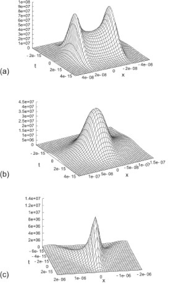
Figure 4: The amplitude distribution $|{\vec{E_{x}}}|$, in the arbitrary units, at the three distances $z$ from the screen: (a) - $(z=-0.1a)$, (b) - $(z=-a)$ and (c) - $(z=-10a)$. Here, the incident-pulse duration $\tau=2$fs, the aperture width $2a=50$nm and thickness $b=25$nm, the packet central wavelength $\lambda_{0}=500$nm and the amplitude $U(x,z=b)=1$. The time $t$ and coordinate $x$ are in the second and meter units, respectively.

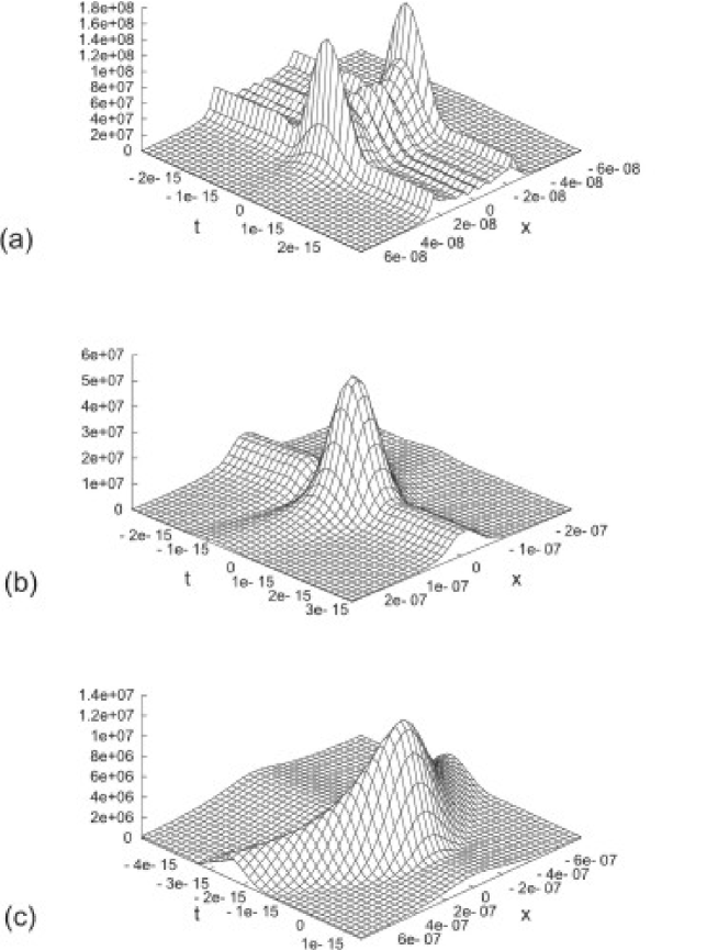
Figure 5: The amplitude distribution $|{\vec{E_{x}}}|$, in the arbitrary units, at the three distances $z$ from the screen: (a) - $(z=-0.1a)$, (b) - $(z=-a)$ and (c) - $(z=-10a)$. Here, the incident-pulse duration $\tau=750$as, the aperture width $2a=50$nm and thickness $b=25$nm, the packet central wavelength $\lambda_{0}=500$nm and the amplitude $U(x,z=b)=1$. The time $t$ and coordinate $x$ are in the second and meter units, respectively.

- (1) D.W. Pohl, D. Courjon, Eds., Near Field Optics, NATO ASI Series E Vol. 242 (The Netherlands, Dordrecht: Kluwer, 1993).
- (2) M. Nieto-Vesperinas, N. Garcia, Eds., Optics at the Nanometer Scale (The Netherlands, Dordrech: Kluwer, 1996).
- (3) A. Lewis, in Current Trends in Optics, J.C. Dainty, Ed., (New York: Academic Press, 1994) pp. 250-253.
- (4) E.Betzig, R.J. Chichester, Science 262, 1422 (1994).
- (5) X.S. Xie, R.C. Dunn, Science 265, 361 (1994).
- (6) W.P. Ambrose, P.M. Goodwin, J.C. Martin, R.A. Keller, Science 265, 364 (1994).
- (7) A. Nahata, T.F. Heinz, IEEE J. Sel. Top. Quantum Electron. 2, 701 (1996).
- (8) J. Bromage, S. Radic, G.P. Agrawal, C.R. Stroud, Jr.P.M. Fauchet, R. Sobolevski, J. Opt. Soc. Am. B 15, 1399 (1998).
- (9) O. Mitrofanov, M. Lee, J.W.P. Hsu, L.N. Pleiffer, K.W. West, J.D. Wynn, J. Federici, Appl. Phys. Lett. 79, 907 (2001).
- (10) O. Mitrofanov, M. Lee, L.N. Pleiffer, K.W. West, Appl. Phys. Lett. 80, 1319 (2002).
- (11) S.V. Kukhlevsky, G. Nyitray, J. Opt. A: Pure Appl. Opt. 4, 271 (2002).
- (12) P.M. Paul, E.S. Toma, P. Breger, G. Mullot, F. Auge, P. Balcou, H.G. Muller, P. Agostini, Science 292, 1689 (2001).
- (13) M. Hentschel, R. Kienberger, Ch. Spielmann, G.A. Reider, N. Milosevic, T. Brabec, P.B. Corcum, U. Heinzmann, M. Drecher, F. Krausz, Nature 414, 509 (2001).
- (14) A.E. Kaplan, P.L. Shkolnikov, Phys. Rev. Lett. 88, 074801-4 (2001).
- (15) F. L. Neerhoff, G. Mur G, Appl. Sci. Res. 28, 73 (1973).
- (16) E. Betzig, A. Harootunian, A. Lewis, M. Isaacson, Appl. Opt. 25, 1890 (1986).
- (17) R.F. Harrington, D.T. Auckland, IEEE Trans. Antennas Propag. AP-28, 616 (1980).
- (18) S.V. Kukhlevsky, Europhys. Lett. 54, 461 (2001).
- (19) L. Novotny, D.W. Pohl, P. Regli, J. Opt. Soc. Am. A 11, 1768 (1994).
- (20) C. Girard, O.J.F. Martin, A. Dereux, Phys. Rev. Lett. 75, 3098 (1995).
- (21) K. Wynne, Opt. Commun. bf209, 85 (1995).