Prediction and statistics of pseudoknots in RNA structures
using exactly clustered stochastic simulations

Ab initio RNA secondary structure predictions have long dismissed helices interior to loops, so-called pseudoknots, despite their structural importance. Here, we report that many pseudoknots can be predicted through long time scales RNA folding simulations, which follow the stochastic closing and opening of individual RNA helices. The numerical efficacy of these stochastic simulations relies on an ${\cal\bf O}(n^{2})$ clustering algorithm which computes time averages over a continously updated set of $n$ reference structures. Applying this exact stochastic clustering approach, we typically obtain a 5- to 100-fold simulation speed-up for RNA sequences up to 400 bases, while the effective acceleration can be as high as 10⁵-fold for short multistable molecules ($\leq$ 150 bases). We performed extensive folding statistics on random and natural RNA sequences, and found that pseudoknots are unevenly distributed amongst RNA structures and account for up to 30% of base pairs in G+C rich RNA sequences (Online RNA folding kinetics server including pseudoknots : http://kinefold.u-strasbg.fr/).

The folding of RNA transcripts is driven by intramolecular GC/AU/GU base pair stacking interactions. This primarily leads to the formation of short double-stranded RNA helices connected by unpaired regions. Ab initio RNA folding prediction restricted to tree-like secondary structures is now well establishednussinov ; waterman ; nussinov2 ; zuker ; mccaskill ; turner ; vienna ; higgs and has become an important tool to study and design RNA structures which remain by and large refractory to many crystallization techniques. Yet, the accuracy of these predictions is difficult to assess –despite the precision of stacking interaction tablesturner – due to their a priori dismissal of pseudoknot helices, Fig 1A.

Pseudoknots are regular double-stranded helices which provide specific structural rigidity to the RNA molecule by connecting different “branches” of its otherwise more flexible tree-like secondary structure (Figs 1A-B). Many ribozymes, which require a well-defined 3D enzymatic shape, have pseudoknotspleij ; tinoco ; westhof ; williamson1 ; woodson1 ; williamson2 ; woodson2 ; herschlag ; ferre . Pseudoknots are also involved in mRNA-ribosome interactions during translation initiation and frameshift regulationframeshift . Still, the overall prevalence of pseudoknots has proved difficult to ascertain from the limited number of RNA structures known to date. This has recently motivated several attempts to include pseudoknots in RNA secondary structure predictionsgultyaev ; eddy ; isambert .

There are two main obstacles to include pseudoknots in RNA structures: a structural modeling problem and a computational efficiency issue. In the absence of data bases for pseudoknot energy parameters, their structural features have been modeled at various descriptive levels using polymer theorymironov ; gultyaev ; isambert . From a computational perspective, pseudoknots have proved not easily amenable to classical polynomial minimization algorithmseddy due to their intrinsic non-nested nature. Instead, simulating RNA folding dynamics has provided an alternative avenue to predict pseudoknotsmironov ; isambert in addition to bringing some unique insight into the kinetic aspects of RNA foldinghiggs ; isambert .

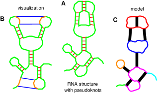
Figure 1: A An RNA secondary structure with pseudoknots. B Minimum set of helices defined as “pseudoknots” and visualized for convenience by colored single-stranded regions connected by two straight lines. C The entropic cost of the actual 3D structural constraints is evaluated by modeling RNA helices as stiff rods (black) and single-stranded regions as ideal polymer springs. Colored single-stranded circuits define quasi-independent structural domains referred to as “nets” in refisambert .

Yet, stochastic RNA folding simulations can become relatively inefficient due to the occurrence of short cycles amongst closely related configurationsmironov , which typically differ by a few helices only. Not surprisingly, similar numerical pitfalls have been recurrent in stochastic simulations of other trapped dynamical systemsfrenkel ; BKL ; mezard ; voter ; pande .

To address this computational efficiency issue and capture the slow folding dynamics of RNA molecules, we have developed a generic algorithm which greatly accelerates RNA folding stochastic simulations by exactly clustering the main short cycles along the explored folding paths. The general approach, which may prove useful to simulate other trapped dynamical systems, is discussed in the main subsection of Theory and Methods. In the Results section, the efficacy of these exactly clustered stochastic (ECS) simulations is first compared to non-clustered RNA folding simulations, before being used to predict the prevalence of pseudoknots in RNA structures on the basis of the structural model introduced in refisambert and briefly reviewed hereafter.

Theory and Methods

Modeling and visualizing pseudoknots in RNA structures. We model the 3D constraints associated with pseudoknots using polymer theory. The entropy costs of pseudoknots and internal, bulge and hairpin loops are evaluated on the same basis by modeling the secondary structure (including pseudoknots) as an assembly of stiff rods –representing the helices– connected by polymer springs –corresponding to the unpaired regions, Fig 1C. In practice, free energy computations involve the labelling of RNA structures into constitutive “nets” –shown as colored circuits on Fig 1C– to account for the stretching of the unpaired regions linking the extremities of pseudoknot helices, see refisambert for details. In addition, free energy contributions from base pair stackings, terminal mismatches and co-axial stackings are taken from the thermodynamic tables measured by the Turner labturner .

The main limitation of this structural model is the absence of hardcore interactions, which could stereochemically prohibit certain RNA structures with either long pseudoknots (e.g., $>$11bp, one helix turn) or a large proportion of pseudoknots (e.g., $>$30% of formed base pairs). However, we found that such stereochemically improbable structures account for less than 1-to-10% of all predicted structures, depending on G+C content (see Results section). Hence, in practice, neglecting hardcore interactions is rarely a stringent limitation, except for a few, somewhat pathological cases.

Although the presence of pseudoknots in an RNA structure is not associated to a unique set of helices, it is convenient for visualization and statistics purposes to define the set of pseudoknots as the minimum set of helices which should be imagined broken to obtain a tree-like secondary structure, Fig 1B. Finding such a minimum set (with respect to the number of base pairs or their free energy) amounts to finding the maximum tree-like set amongst the formed helices and can be done in polynomial time using a classical “dynamic programming” algorithm.

Modeling RNA folding dynamics and straightforward stochastic algorithm. RNA folding kinetics is known to proceed through rare stochastic openings and closings of individual RNA helicesporschke74bonnet98 . The time limiting step to transit between two structures sharing essentially all but one helix can be assigned Arrhenius-like rates, $k_{\pm}=k^{\circ}\times\exp(-\Delta G_{\pm}/kT)$, where $kT$ is the thermal energy. $k^{\circ}$, which reflects only local stacking processes within a transient nucleation core, has been estimated from experiments on isolated stem-loopsporschke74bonnet98 ($k^{\circ}\simeq 10^{8}$ s^-1), while the free energy differences $\Delta G_{\pm}$ between the transition states and the current configurations (Fig 2) can be evaluated by combining the stacking energy contributions and the global coarse-grained structural model described above, Fig 1C.

Simulating a stochastic RNA folding pathway amounts to following one particular stochastic trajectory within the large combinatorial space of mutually compatible helicesmironov . Each transition in this discrete space of RNA structures corresponds to the opening or closing of a single helix, possibly followed by additional helix elongation and shrinkage rearrangements to reach the new structure’s equilibrium compatible with a minimum size constraint for each formed helixisambert (base pair zipping/unzipping kinetics occurs on much shorter time scales than helix nucleation/dissociation). For a given RNA sequence, the total number of possible helices (which roughly scales as $L^{2}$, where $L$ is the sequence length) sets the local connectivity of the discrete structure space and therefore the number of possible transitions from each particular structure.

Formally, we consider the following generic model. Each structure or “state” $i$ is connected to a finite, yet possibly state-to-state varying number of neighboring configurations $j$ via transition rates $k_{ji}$ (the right-to-left matrix ordering of indices is adopted hereafter). As $k_{ji}$ is the average number of transitions from state $i$ to state $j$ per unit time, the lifetime $t_{i}$ of configuration $i$ corresponds to the average time before any transition towards a neighboring state $j$ occurs, i.e., $t_{i}=1/{\sum_{\langle j\rangle}}k_{ji}$, and the transition probability from state $i$ to state $j$ is $p_{ji}=k_{ji}t_{i}$, with ${\sum_{\langle j\rangle}}p_{ji}=1$, as expected, for all state $i$.

Figure 2: Stochastic transitions over a thermodynamic barrier $\Delta G_{\pm}$ to close and open an individual helix between two neighbor RNA structures, $i$ and $j$. Nucleation of the new helix usually involve some local unzipping of nearby helices at the barrier and further base pair rearrangements to reach equilibrium in the new structure $j$isambert .

Hence, in the straightforward stochastic algorithmmironov ; isambert , each new transition is picked at random with probability $p_{ji}$ while the effective time is incremented with the lifetime $t_{i}$ of the current configuration $i$distribution . However, as mentioned in the introduction, the efficiency of this approach is often severely impeded by the existence of kinetic traps consisting of rapidly exchanging states.

Exactly clustered stochastic (ECS) simulations. As in the case of RNA folding dynamics, the simulation of other trapped dynamical systems generally presents a computational efficiency issue. In particular, powerful numerical schemes have been developed to compute the elementary escape times from traps for a variety of simulation techniquesfrenkel ; BKL ; mezard ; voter ; pande . Still a pervasive problem usually remains for most applications due to the occurrence of short cycles amongst trapped states, and heuristic clustering approaches have been proposed to overcome these “numerical traps”krauth .

To capture the slow folding dynamics of RNA molecules, we have developed an exact stochastic algorithm which accelerates the simulation by numerically integrating the main short cycles amongst trapped states. This approach being quite general, it could prove useful to simulate other small, trapped dynamical systems with coarse-grained degrees of freedom.

In a nutshell, the ECS algorithm aims at overcoming the numerical pitfalls of kinetic traps by “clustering” some recently explored configurations into a single, yet continuously updated cluster $A$ of $n$ reference states. These clustered configurations are then collectively revisited in the subsequent stochastic exploration of states. Although stochasticity is “lost” for the individual clustered states, its statistical properties are, however, exactly transposed at the scale of the set $A$ of the $n$ reference states. This is achieved as follows. For each pathway $C^{A}_{m}$ on $A$, a statistical weight $W^{C^{A}_{m}}=\prod^{C^{A}_{m}}p_{lk}$ is defined, where $k$ and $l$ run over all consecutive states along $C^{A}_{m}$ from its “starting” state $i$ to its “exiting” state $j$ on $A$. The $n\!\times\!n$ probability matrix $P^{A}$ which sums the statistical weights $W^{C^{A}_{m}}$ over all pathways $C^{A}_{m}$ on $A$ between any two states $i$ and $j$ of $A$ is then introduced,

$$P^{A}_{ji}=\sum^{C^{A}}_{m:j\leftarrow i}W^{C^{A}_{m}}=\sum^{C^{A}}_{m:j\leftarrow i}\biggl{(}\ \prod_{j\leftarrow i}^{C^{A}_{m}}p_{lk}\biggr{)},$$ (1)

and the exit probability to make a transition outside $A$ from the state $j$ is noted: $p^{eA}_{j}=1-{\sum^{A}_{\langle k\rangle}}p_{k}j$. Hence, starting from state $i$, the probability to exit the set $A$ at state $j$ is $p^{eA}_{j}P^{A}_{ji}$, with $\sum^{A}_{j}p^{eA}_{j}P^{A}_{ji}=1$, for all $i$ of $A$.

Thus, in the ECS algorithm, one first chooses at random with probability $p^{eA}_{j}P^{A}_{ji}$ the reference state $j$ of $A$ from which a new transition towards a state $k$ outside $A$ will then be chosen stochastically with probability $p_{kj}/p^{eA}_{j}$. Meanwhile, the physical quantities of interest, like the cumulative time lapse ${t}^{A}_{ji}$ to exit the set $A$ from $j$ starting at $i$, are exactly averaged over all (future) pathways from $i$ to $j$ within $A$, as explained in the next subsection. Finally, the new state $k$ is added to the reference set $A$ whilst another reference state is removed, so as to update $A$, as discussed in The ${\cal O}(n^{2})$ algorithm subsection.

Exact averaging over all future pathways. We start the discussion with the path average time lapse to exit the set $A$. Let us introduce the time lapse transform of ${P}^{A}$: ${\cal T}[{P}^{A}]\{t\}=\tilde{P}^{A}\{t\}$, which sums the weighted cumulative lifetimes $\bigl{(}\sum^{C^{A}_{m}}t_{h}\bigr{)}\prod^{C^{A}_{m}}p_{lk}$ over all pathways $C^{A}_{m}$ on $A$ between any two states $i$ and $j$ of $A$,

$${\cal T}[{P}^{A}]_{ji}\{t\}=\tilde{P}^{A}_{ji}\{t\}=\sum^{C^{A}}_{m:j\leftarrow i}\Biggl{[}\biggl{(}\sum_{j\leftarrow i}^{C^{A}_{m}}t_{h}\biggr{)}\prod_{j\leftarrow i}^{C^{A}_{m}}p_{lk}\Biggr{]},$$ (2)

where the $t_{h}$’s are summed over all consecutive states $h$ –from $i$ to $j$ included– along each pathway $C^{A}_{m}$. Hence, the mean time $\bar{t}^{A}_{i}$ to exit $A$ from any state $j$ of $A$ starting from configuration $i$ is, $\bar{t}^{A}_{i}=\sum^{A}_{j}p^{eA}_{j}\tilde{P}^{A}_{ji}\{t\}$. However, in the context of the ECS algorithm, the time lapse of interest is $\bar{t}^{A}_{ji}$, the mean time to exit $A$ from a particular state $j$, $\bar{t}^{A}_{ji}={p^{eA}_{j}\tilde{P}^{A}_{ji}\{t\}/p^{eA}_{j}P^{A}_{ji}}={\tilde{P}^{A}_{ji}\{t\}/P^{A}_{ji}}$.

The average of any path cumulative quantity of interest $x_{i}$ can be similarly obtained by introducing the appropriate $\tilde{P}^{A}\{x\}$ matrix. In particular, the instantaneous efficiency of the algorithm is well reflected by the average pathway length $\bar{\ell}^{A}_{ji}$ between any two states of $A$,

$$\bar{\ell}^{A}_{ji}={\tilde{P}^{A}_{ji}\{\ell\}/P^{A}_{ji}},$$ (3)

where $\tilde{P}^{A}_{ji}\{\ell\}=\sum^{C^{A}}_{m:j\leftarrow i}\bigl{[}\bigl{(}\sum^{C^{A}_{m}}1\bigr{)}\prod^{C^{A}_{m}}p_{lk}\bigr{]}$, with $\sum^{C^{A}_{m}}1$ corresponding to the length of the pathway $C^{A}_{m}$ (1 is added at each state along each pathway $C^{A}_{m}$). Hence, starting from state $i$, $\bar{\ell}^{A}_{ji}$ corresponds to the average number of transitions that would have to be performed by the straightforward algorithm before exiting the set $A$ at state $j$. As expected, $\bar{\ell}^{A}_{ji}$ can be very large for a trapped dynamical system, which accounts for the efficiency of the present algorithm. Since the approach is exact, there is, however, no a priori requirement on the trapping condition of the states of $A$ and the algorithm can be used continuously.

Similarly, the time average of any physical quantity $y_{i}$ –like the pseudoknot proportion of an RNA molecule– can be calculated by introducing the appropriate time weighted matrix $\tilde{P}^{A}\{yt\}$. For instance, the time average energy $\bar{E}^{A}_{ji}$ over all pathways between any two states $i$ and $j$ of $A$ is, $\bar{E}^{A}_{ji}={\tilde{P}^{A}_{ji}\{Et\}/\tilde{P}^{A}_{ji}\{t\}}$, where $\tilde{P}^{A}_{ji}\{Et\}=\sum^{C^{A}}_{m:j\leftarrow i}\bigl{[}\bigl{(}\sum^{C^{A}_{m}}E_{h}t_{h}\bigr{)}\prod^{C^{A}_{m}}p_{lk}\bigr{]}$.

The actual calculation of the probability and path average matrices $P^{C}$ and $\tilde{P}^{C}$ over a set $C$ of $N$ states will be performed recursively in the next subsection. As an intermediate step, we first consider hereafter the unidirectional connection between two disjoint sets $A$ and $B$.

Let us hence introduce the transfer matrix $T^{BA}$ from set $A$ to set $B$ defined as $T^{BA}_{ji}=p_{ji}$, where $p_{ji}$ is the probability to make a transition from state $i$ of $A$ to state $j$ of $B$ ($T^{BA}_{ji}=0$ if $i$ and $j$ are not connected). We will assume that $A$ has $n$ states and $B$ $m$ states and that their probability and path average matrices $P^{A}$, $\tilde{P}^{A}$, $P^{B}$ and $\tilde{P}^{B}$ are known. Starting at state $i$ of $A$, we find that the probability to exit on $j$ of $B$ after crossing once and only once from $A$ to $B$ is, $p^{eB}_{j}(P^{B}T^{BA}P^{A})_{ji}$, where we have used matrix notations. Let us consider a particular path from $i$ in $A$ to $j$ in $B$ crossing once and only once from $A$ to $B$, with statistical weight $\bigl{(}\prod^{B}p_{lk}\bigr{)}p_{ba}\bigl{(}\prod^{A}p_{l^{\prime}k^{\prime}}\bigr{)}$. Its contribution to the average time to exit somewhere from the union of $A$ and $B$ is,

$$\!\!\biggl{(}\sum_{j\leftarrow b}^{B}t_{h}+\sum_{a\leftarrow i}^{A}t_{h^{\prime}}\biggr{)}\prod_{j\leftarrow b}^{B}p_{lk}\cdot p_{ba}\cdot\prod_{a\leftarrow i}^{A}p_{l^{\prime}k^{\prime}}=$$ (4)

$$\!\!\biggl{(}\sum_{j\leftarrow b}^{B}\!t_{h}\prod_{j\leftarrow b}^{B}p_{lk}\!\biggr{)}p_{ba}\prod_{a\leftarrow i}^{A}p_{l^{\prime}k^{\prime}}\!+\!\prod_{j\leftarrow b}^{B}p_{lk}\ p_{ba}\biggl{(}\sum_{a\leftarrow i}^{A}\!t_{h^{\prime}}\!\prod_{a\leftarrow i}^{A}p_{l^{\prime}k^{\prime}}\!\!\biggr{)}$$

or in matrix form for any “direct” pathway from $A$ to $B$,

$${\cal T}[{P^{B}T^{BA}P^{A}}]={\cal T}[{P}^{B}]\ T^{BA}P^{A}+P^{B}T^{BA}{\cal T}[{P}^{A}],$$ (5)

which implies that applying the usual differentiation rules to any combination of probability matrices yields the correct combined path average matrices (defining ${\cal T}[{T}^{BA}]_{ij}=0$ for all $i$ and $j$). Note, this out-of-equilibrium calculation of path average quantities is reminiscent of the usual equilibrium calculation of thermal averages through differentiation of an appropriate Partition Function. Indeed, the probability matrices introduced here are “partition functions” over all pathways within a set of reference states.

The ${\cal O}(n^{2})$ algorithm. With this result in mind, we can now return to the calculation of the probability and path average matrices $P^{C}$ and $\tilde{P}^{C}$ for the union $C$ of two disjoint sets $A$ and $B$.

Defining $P^{Ab}\!\!=\!P^{A}T^{AB}\!$ and $P^{Ba}\!\!=\!P^{B}T^{BA}\!$, we readily obtain the probability matrix $P^{C}$ as an infinite summation over all possible pathway loops between the sets $A$ and $B$ (${I}$ is the identity matrix),

$$P^{C~{}}= \left(\begin{array}[]{c}Q^{AA}\,\,\,Q^{AB}\\ Q^{BA}\,\,\,Q^{BB}\end{array}\right),\,\,\,{\rm with}$$

$$Q^{AA}= \bigl{[}{I}\!+\!P^{Ab}P^{Ba}\!+\!(P^{Ab}P^{Ba})^{2}\!+\!\cdots\bigr{]}P^{A}\!=\!L^{A}P^{A}$$

$$Q^{BA}= P^{Ba}L^{A}P^{A}$$

$$Q^{BB}= \bigl{[}{I}\!+\!P^{Ba}P^{Ab}\!+\!(P^{Ba}P^{Ab})^{2}\!+\!\cdots\bigr{]}P^{B}\!=\!L^{B}P^{B}$$

$$Q^{AB}= P^{Ab}L^{B}P^{B}$$

where $L^{A}\!=\![{I}-P^{Ab}P^{Ba}]^{-1}$ and $L^{B}\!=\![{I}-P^{Ba}P^{Ab}]^{-1}$.

Defining also $\tilde{P}^{Ab}=\tilde{P}^{A}T^{AB}$ and $\tilde{P}^{Ba}=\tilde{P}^{B}T^{BA}$, we finally obtain the path average matrix $\tilde{P}^{C}$ from simple “differentiation” of the “partition function” ${P}^{C}$, Eqs.(Prediction and statistics of pseudoknots in RNA structures using exactly clustered stochastic simulations),

$$\tilde{P}^{C~{}}= \left(\begin{array}[]{c}\tilde{Q}^{AA}\,\,\,\tilde{Q}^{AB}\\ \tilde{Q}^{BA}\,\,\,\tilde{Q}^{BB}\end{array}\right),\,\,\,{\rm with}$$

$$\tilde{Q}^{AA}= \tilde{L}^{A}P^{A}+L^{A}\tilde{P}^{A}$$

$$\tilde{Q}^{BA}= \tilde{P}^{Ba}L^{A}P^{A}+P^{Ba}\tilde{L}^{A}P^{A}+P^{Ba}L^{A}\tilde{P}^{A}$$

$$\tilde{Q}^{BB}= \tilde{L}^{B}P^{B}+L^{B}\tilde{P}^{B}\hskip 93.89418pt$$

$$\tilde{Q}^{AB}= \tilde{P}^{Ab}L^{B}P^{B}+P^{Ab}\tilde{L}^{B}P^{B}+P^{Ab}L^{B}\tilde{P}^{B}$$

$$\rm where, \tilde{L}^{A}=L^{A}\bigl{(}\tilde{P}^{Ab}P^{Ba}+P^{Ab}\tilde{P}^{Ba}\bigr{)}L^{A}$$

$$\rm and \tilde{L}^{B}=L^{B}\bigl{(}\tilde{P}^{Ba}P^{Bb}+P^{Ba}\tilde{P}^{Ab}\bigr{)}L^{B}$$

Eqs.(Prediction and statistics of pseudoknots in RNA structures using exactly clustered stochastic simulations) and (Prediction and statistics of pseudoknots in RNA structures using exactly clustered stochastic simulations) are valid for any sizes $n$ and $m$ of $A$ and $B$. Hence $P^{C}$ and $\tilde{P}^{C}$ can be calculated recursively starting from $N$ isolated states and $2N$ $1\!\times\!1$ matrices $P^{i}=[1]$ and $\tilde{P}^{i}\{x\}=[x_{i}]$, with $i=1,N$, where $x_{i}$ is the value of the feature of interest in state $i$. Clustering those states 2 by 2, then 4 by 4, etc…, using Eqs.(Prediction and statistics of pseudoknots in RNA structures using exactly clustered stochastic simulations) and (Prediction and statistics of pseudoknots in RNA structures using exactly clustered stochastic simulations) finally yields $P^{C}$ and $\tilde{P}^{C}$ in ${\cal O}(N^{3})$ operations (i.e., by matrix inversions and multiplications). However, instead of recalculating everything back recursively from scratch each time the set of reference states is modified, it turns out to be much more efficient to update it continuously each time a single state is added. Indeed, Eqs.(Prediction and statistics of pseudoknots in RNA structures using exactly clustered stochastic simulations) and (Prediction and statistics of pseudoknots in RNA structures using exactly clustered stochastic simulations) can be calculated in ${\cal O}(n^{2})$ operations only, when $m=1$ and $n=N\!-\!1$, as we will show below. Naturally, a complete update also requires the removal of one “old” reference state each time a “new” one is added, so as to keep a stationary number $n$ of reference configurations. As we will see, this removal step can also be calculated in ${\cal O}(n^{2})$ operations only.

The ${\cal O}(n^{2})$-operation update of the reference set, which we now outline, relies on the fact that $T^{AB}$, $P^{Ab}$ and $\tilde{P}^{Ab}$ are $n\!\times\!1$ matrices and that $T^{BA}$, $P^{Ba}$ and $\tilde{P}^{Ba}$ are $1\!\times\!n$ matrices, when $m=1$ and $n=N\!-\!1$ ($P^{B}$ and $L^{B}$ are simple $1\!\times\!1$ matrices for a single state $B$). Since we operate on vectors, the Sherman-Morrison formulanumrec can then be used to calculate the $n\!\times\!n$ matrix $L^{A}=\bigl{[}{I}-P^{Ab}\otimes P^{Ba}\bigr{]}^{-1}=\bigl{[}{I}+P^{Ab}\otimes P^{Ba}/(1-P^{Ab}\cdot P^{Ba})\bigr{]}$. Hence, not only $L^{A}$ but also any matrix product $L^{A}M$, where $M$ is a $n\!\times\!n$ matrix, can be evaluated in ${\cal O}(n^{2})$ operations [by first calculating $P^{Ba}M$ followed by $P^{Ab}\otimes(P^{Ba}M)$]. Noticing that the same reasoning applies for the $n\!\times\!n$ matrices $\tilde{P}^{Ab}\otimes P^{Ba}$ and $P^{Ab}\otimes\tilde{P}^{Ba}$ provides a simple scheme to add a single reference state to $A$ and obtain matrices $P^{C}$ and $\tilde{P}^{C}$ in ${\cal O}(n^{2})$ operations using Eqs.(Prediction and statistics of pseudoknots in RNA structures using exactly clustered stochastic simulations) and (Prediction and statistics of pseudoknots in RNA structures using exactly clustered stochastic simulations).

In order to achieve the reverse modification consisting in removing one state $B$ from the reference set $C$, it is useful to first imagine that the original $P^{C}$ and $\tilde{P}^{C}$ were obtained by the addition of the single state $B$ to the $n$-configuration set $A$, as given by Eqs.(Prediction and statistics of pseudoknots in RNA structures using exactly clustered stochastic simulations) and (Prediction and statistics of pseudoknots in RNA structures using exactly clustered stochastic simulations). Identifying row $Q^{BA}$, column $Q^{AB}$ and their intersection $Q^{BB}$ corresponding to the single state $B$ readily yields the vectors $P^{Ab}\!=Q^{AB}/Q^{BB}$, $P^{Ba}\!=T^{BA}$ (as $P^{B}=[1]$) and, hence, the $n\!\times\!n$ matrix $[L^{A}]^{-1}={I}-P^{Ab}\otimes P^{Ba}=$ ${I}-(Q^{AB}\otimes T^{BA})/Q^{BB}$. This gives the following relations between the known $L^{A}$, $T^{AB}$, $T^{BA}$, $Q^{AA}$, $Q^{BB}$, $Q^{BA}$, $Q^{AB}$, $\tilde{P}^{B}$ and $\tilde{Q}^{AA}$, and the unknown $P^{A}$ and $\tilde{P}^{A}$,

$$Q^{AA} \!\!=L^{A}P^{A},$$

$$\tilde{Q}^{AA} \!\!=L^{A}\!\Bigl{[}\tilde{P}^{A}\bigl{(}{I}+T^{AB}\!\otimes Q^{BA}\bigl{)}+{\tilde{P}^{B}\over Q^{BB}}Q^{AB}\!\otimes Q^{BA}\Bigr{]}$$

which eventually provides $P^{A}$ and $\tilde{P}^{A}$ using the Sherman-Morrison formulanumrec to invert ${I}+T^{AB}\otimes Q^{BA}$,

$$P^{A} \!\!=[L^{A}]^{-1}Q^{AA}=\Bigl{(}{I}-{Q^{AB}\otimes T^{BA}\over Q^{BB}}\Bigr{)}Q^{AA},$$ (13)

$$\tilde{P}^{A} \!\!=\!\Bigl{[}\!\Bigl{(}\!{I}\!-{Q^{AB}\!\otimes T^{BA}\over Q^{BB}}\Bigr{)}\tilde{Q}^{AA}\!-{\tilde{P}^{B}\over Q^{BB}}Q^{AB}\!\otimes Q^{BA}\Bigr{]}\!\times$$

$$\hskip 8.5359pt\Bigl{(}{I}-{T^{AB}\otimes Q^{BA}\over 1-T^{AB}\cdot Q^{BA}}\Bigr{)}$$

Hence, the single state $B$ can be removed from the set of reference $C$ in ${\cal O}(n^{2})$ operations to yield the updated probability and path average matrices $P^{A}$ and $\tilde{P}^{A}$.

Note, however, that this continuous updating procedure, using alternatively Eqs.(Prediction and statistics of pseudoknots in RNA structures using exactly clustered stochastic simulations,Prediction and statistics of pseudoknots in RNA structures using exactly clustered stochastic simulations) and Eqs.(13,13) in succession, is expected to become numerically unstable after too many updates of the reference set. For $1\leq n\leq 300$, we have usually found that the small numerical drifts [as measured e.g. by $\epsilon=\sum^{A}_{i}(\sum^{A}_{j}p^{eA}_{j}P^{A}_{ji}-1)^{2}\simeq 0$] can simply be reset every $n^{\rm th}$ update by recalculating matrices $P^{A}$ and $\tilde{P}^{A}$ recursively from $n$ isolated states in ${\cal O}(n^{3})$ operations, so as to keep the overall ${\cal O}(n^{2})$-operation count per update of the reference set.

Another important issue is the choice of the state to be removed from the updated reference set. Although this choice is in principle arbitrary, the benefit of the algorithm strongly hinges on it (for instance removing one of the most statistically visited reference states usually ruins the efficiency of the method). We have found that a “good choice” is often the state $j^{\star}$ with the lowest “exit frequency” from the current state $i$ [i.e., $1/\bar{t}^{A}_{j^{\star}i}=\min^{A}_{j}\!(1/\bar{t}^{A}_{ji})$], but other choices may sometimes prove more appropriate.

Results

Performance of the ECS algorithm. Before applying the ECS algorithm to investigate the prevalence of pseudoknots in RNA structures, we first focus on the efficacy of the approach by studying the net speed-up of the ECS algorithm with respect to the straightforward algorithm. As illustrated on Fig 3 for a few natural and artificial sequences, there is an actual $10^{1}$ to $10^{5}$-fold increase of the ratio “simulated-time over CPU-time” between ECS and straightforward algorithms (black lines) for RNA shorter than about $150$ nt, Fig 3. This improvement runs parallel to the expected speed-up (grey lines) as predicted by $\bar{\ell}^{A}_{ji}$, Eq.(3), as long as the number $n$ of reference states is not too large (typically $n\leq 50$ here), so that the ${\cal O}(n^{2})$ update routines do not significantly increase the operation count as compared to the straightforward algorithm.

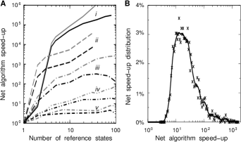
Figure 3: A: Expected (grey lines) and actual (black lines) speed-up of the approach with respect to the straightforward algorithm (see main text). i: Bistable molecule in Fig 4C (with a combinatorial structure space of 37 possible helices); ii: 67-nt-long molecule with reverse sequence of the bistable molecule in Fig 4C (38 possible helices). The ${\cal O}(n^{2})$ algorithm becomes unstable above 40 reference states in this case (see main text); iii: Hepatitis delta virus ribozyme, Fig 4B (84 possible helices); iv: average speed-up for random 100-nt-long RNA sequences with 50% G+C content. v: Group I intron ribozyme, Fig 4A (894 possible helices). B: Net speed-up distribution amongst random 100-nt-long RNA sequences with 50% G+C content (iv on Fig 3A) for a cluster of 40 reference states.

Hence, the ECS algorithm is most efficient for small trapped systems (when the dynamics can be appropriately coarse-grained), although a several-fold speed-up can still be expected with somewhat larger systems, such as the 394-nt-long Group I intron pictured in Fig 4A.

Alternatively, using this exact approach may also provide a controlled scheme to obtain approximate coarse-grained dynamics for larger systems. The C routines of the ECS algorithm are freely available upon request.

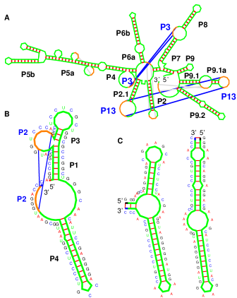
Figure 4: RNA structure prediction with the ECS algorithm. Structures are drawn using the “RNAMovies” softwareevers adapted to visualize predicted pseudoknots. A 394-base long Tetrahymena Group I intron: the lowest free-energy structure found shares 80% base pair identity with the known 3D structure, including the two main pseudoknots, P3 and P13westhof ; williamson1 ; woodson1 ; williamson2 ; woodson2 ; herschlag . B 88-base long hepatitis delta virus ribozyme: predicted structure shares 93% base pair identity with the known 3D structure, including the main pseudoknot P2isambert (but not the 2-base pair long P1.1ferre ); C The two structures of a bistable, 67-nt-long artificial RNA molecule.

Pseudoknot prediction and prevalence in RNA structures. In the context of RNA folding dynamics, the present approach can be used to evaluate time averages for a variety of physical features of interest, such as the free energy along the folding paths, the fraction of time particular helices are formed, the extension of an RNA molecule unfolding under mechanical forceharlepp , the end-to-end distance of a nascent RNA molecule during transcription, etc. Here, we report results on the prediction of pseudoknot prevalence in RNA structures. They have been obtained performing several thousands of stochastic RNA folding simulations including pseudoknots. As explained in Theory and Methods, the structural constraints between pseudoknot helices and unpaired connecting regions are modeled using elementary polymer theory (Fig 1C,isambert ) and added to the traditional base pair stacking interactions and simple loops’ contributionsturner .

We found that many pseudoknots can effectively be predicted with such a coarse-grained kinetic approach probing seconds to minutes folding time scales. No optimum “final” structure is actually predicted, as such, in this folding kinetic approach. Instead, low free-energy structures are repeatedly visited, as helices stochastically form and break. Fig 4A represents the lowest free-energy secondary structure found for 394-nt-long Tetrahymena Group I intron, which shows 80% base pair identity with the known 3D structure, including the two main pseudoknots, P3 and P13westhof ; williamson1 ; woodson1 ; williamson2 ; woodson2 ; herschlag . A number of smaller known structures with pseudoknots are also compared to the lowest free-energy structures found with similar stochastic RNA folding simulations inisambert . In addition, to facilitate the study of folding dynamics for specific RNA sequences, we have set up an online RNA folding server including pseudoknots at URL http://kinefold.u-strasbg.fr/.

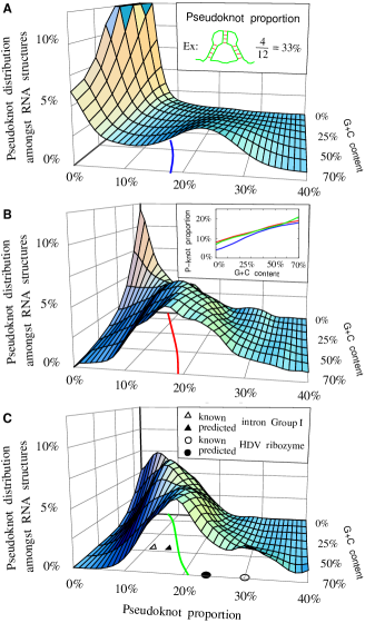
Figure 5: Distribution of pseudoknot proportion amongst formed base pairs for 50-nt-long (A), 100-nt-long (B), and 150-nt-long (C) random sequences of increasing G+C content. Projected lines correspond to the average pseudoknot proportion in 50 (blue), 100 (red), and 150-nt-long (green) random sequences. All three average curves are displayed in inset on Fig 5B. Open (and filled) symbols on Fig 5C correspond to known (and predicted) pseudoknot proportions for Tetrahymena group I intron, Fig 4A (triangles) and Hepatitis delta virus ribozyme, Fig 4Bferre ; isambert (circles).

Beyond specific sequence predictions, we also investigated the general prevalence of pseudoknots by studying the “typical” proportion of pseudoknots in both random RNA sequences of increasing G+C content (Fig 5) and in 150-nt-long mRNA fragments of the Escherichia coli and Saccharomyces cerevisiae genomes. The statistical analysis was done as follows: for each random and genomic sequence set, 100 to 1000 sequences were sampled and 3 independent folding trajectories were simulated for each of them, using the ECS algorithm. A minimum duration for each trajectory was determined so that more than 80-90% of sequences visit the same free-energy minimum structures along their 3 independent trajectories. The time average proportion of pseudoknots was then evaluated, considering this fraction of sequences having likely reached equilibrium (including the 10-20% of still unrelaxed sequences does not significantly affect global statistics). In practice, slow folding relaxation limits extensive folding statistics to sequences up to 150 bases and 75% G+C content, although individual folding pathways can still be studied for molecules up to 250 to 400 bases depending on their specific G+C contents.

The results for 50-nt-long (Fig 5A), 100-nt-long (Fig 5B), and 150-nt-long (Fig 5C) random sequences show, first, a broad distribution in pseudoknot proportion from a few percents of base pairs to more than 30% for some G+C rich random sequences. Such a range is in fact compatible with the various pseudoknot contents observed in different known structures (e.g. see triangles and circles in Fig 5C). Second, the average proportion of pseudoknots (projected curves and inset in Fig 5B) slowly increases with G+C content, since stronger (G+C rich) helices are more likely to compensate for the additional entropic cost of forming pseudoknots. Third, and perhaps more surprisingly, this average proportion of pseudoknots appears roughly independent of sequence length except for very short sequences with low G+C content (inset in Fig 5B), in contradiction with a naive combinatorial argument. Fourth, we found that the cooperativity of secondary structure rearrangements amplifies the structural consequences of pseudoknot formation; typically, a structure with 10 helices including 1 pseudoknot conserves not 9 but only 7 to 8 of its initial helices (while 2 to 3 new nested helices commitantly form) if the single pseudoknot is excluded from the structure prediction. Thus, neglecting pseudoknots usually induces extended structural modifications beyond the sole pseudoknots themselves.

We compared these results with the folding of 150-nt-long sections of mRNAs from the genomes of Escherichia coli (50% G+C content) and Saccharomyces cerevisiae (yeast, 40% G+C content). These genomes exhibit similar broad distributions of pseudoknots, despites small differences due to G+C content inhomogeneity and codon bias usage; pseudoknot proportions (mean $\pm$ std-dev.): E. coli, 15.5$\pm$6.5% (versus 16.5$\pm$7.9% for 50% G+C rich random sequences); yeast, 14$\pm$6.6% (versus 15$\pm$7.3% for 40% G+C rich random sequences); Hence, genomic sequences appear to have maintained a large potential for modulating the presence or absence of pseudoknots in their 3D structures.

Overall, these results suggest that neglecting pseudoknots in RNA structure predictions is probably a stronger impediment than the small intrinsic inaccuracy of stacking energy parameters. In practice, combining simple structural models (Fig 1C) and exactly clustered stochastic (ECS) simulations provides an effective approach to predict pseudoknots in RNA structures.

Acknowledgements

We thank J. Baschenagel, D. Evers, D. Gautheret, R. Giegerich, W. Krauth, M. Mézard, R. Penner, E. Siggia, N. Socci and E. Westhof for discussions and suggestions. Supported by ACI grants n^∘ PC25-01 and 2029 from Ministère de la Recherche, France. H.I. would also like to acknowledge a stimulating two-month visit at the Institute for Theoretical Physics, UCSB, Santa Barbara, where the ideas for this work originated.

References

- (1) Waterman, M.S. (1978) Studies in Found. and Comb., Adv. in Math. Suppl. Stu. 1, 167-212.
- (2) Nussinov, R., Pieczenik, G., Griggs, J.R. & Kleitman D.J. (1978) SIAM J. Appl. Math. 35, 68-82.
- (3) Nussinov, R., & Jacobson, A.B. (1980) Proc. Natl. Acad. Sci. USA 77, 7826-7830.
- (4) Zuker, M. & Stiegler, P. (1981) Nucleic Acids Res. 9, 133-148, and http://bioinfo.math.rpi.edu/mfold/
- (5) McCaskill, J.S. (1990) Biopolymers 29, 1105-1119.
- (6) Hofacker, I.L. , Fontana, W., Stadler, P.F., Bonhoeffer, L.S., Tacker M. & Schuster, P. (1994) Monatsh. Chem. 125, 167-188, and http://www.tbi.univie.ac.at/
- (7) Mathews, D.H., Sabina, J., Zuker, M. & Turner, D.H. (1999) J. Mol. Biol. 288, 911-940.
- (8) Higgs, P.G. (2000) Q. Rev. Biophys. 33, 199-253, and references therein.
- (9) Pleij, C.W.A., Rietveld, K., & Bosch, L. (1985) Nucleic Acids Res. 13, 1717-1731.
- (10) Tinoco, I., Jr. (1997) Nucleic Acids Symp Ser. 36, 49-51.
- (11) Lehnert, V., Jaeger, L., Michel, F. & Westhof, E. (1996) Chem. Biol. 3, 993-1009.
- (12) Zarrinkar, P.P. & Williamson, J.R. (1996) Nature Struc. Biol. 3, 432-438.
- (13) Ferre-D’Amare, A.R., Zhou, K. & Doudna, J.A. (1998) Nature 395, 567-574.
- (14) Sclavi, B., Sullivan, M., Chance, M.R., Brenowitz, M. & Woodson, S.A. (1998) Science 279, 1940-1943.
- (15) Treiber, D.K., Root, M.S., Zarrinkar, P.P. & Williamson, J.R. (1998) Science 279, 1940-1943.
- (16) Pan, J. & Woodson, S.A. (1999) J. Mol. Biol. 294, 955-965.
- (17) Russell, R., Millet, I.S., Doniach, S. & Herschlag, D. (2000) Nature Struc. Biol. 7, 367-370.
- (18) Giedroc, D.P., Theimer, C.A. & Nixon, P.L. (2000) J. Mol. Biol. 298, 167-185. Review.
- (19) Gultyaev, A.P., van Batenburg, E. & Pleij, C.W.A. (1999) RNA 5, 609-617.
- (20) Rivas, E. & Eddy, S.R. (1999) J. Mol. Biol. 285, 2053-2068.
- (21) Isambert, H. & Siggia, E. (2000) Proc. Natl. Acad. Sci. USA 97, 6515-6520.
- (22) Mironov, A.A., Dyakonova, L.P. & Kister, A.E. (1985) J. Biomol. Struct. Dynam. 2, 953-962.
- (23) Frenkel, D. & Smit, B. (1996) Understanding Molecular Simulation (Academic Press) and references therein.
- (24) Bortz, A.B., Kalos, M.H. & Lebowitz, J.L. (1975) J. Comput. Phys. 17, 10.
- (25) Krauth, W. & Mézard, M. (1995) Z. Phys. B 97, 127.
- (26) Voter, A.F. (1998) Phys. Rev. B 57, R13985-R13988.
- (27) Shirts, M.R. & Pande, V.S. (2001) Phys. Rev. Lett. 86, 4983-4987.
- (28) Pörschke, D. (1974) Biophysical Chemistry 1, 381-386.
- (29) Krauth, W. & Pluchery, O. (1994) J. Phys. A; Math. Gen. 27, L715.
- (30) In principle, the approach can be adapted to stochastically drawn lifetimes from known distributions with mean lifetime . This effectively yields a ECS algorithm in this case.
- (31) Press, W.H., Teukolsky, S.A., Veterling, W.T. & Flannery, B.P. (1992) Numerical recipes, 2nd Ed. (University Press, Cambridge).
- (32) Harlepp, S., Marchal, T., Robert, J., Léger, J-F., Xayaphoummine, A., Isambert, H. and Chatenay, D. (2003) http://arxiv.org/physics/0309063
- (33) Evers, D. & Giegerich, R. (1999) Bioinformatics 15, 32-37.