Microscopic study of the He₂-SF₆ trimers

Abstract

The He₂-SF₆ trimers, in their different He isotopic combinations, are studied both in the framework of the correlated Jastrow approach and of the Correlated Hyperspherical Harmonics expansion method. The energetics and structure of the He-SF₆ dimers are analyzed, and the existence of a characteristic rotational band in the excitation spectrum is discussed, as well as the isotopic differences. The binding energies and the spatial properties of the trimers, in their ground and lowest lying excited states, obtained by the Jastrow ansatz are in excellent agreement with the results of the converged CHH expansion. The introduction of the He-He correlation makes all trimers bound by largely suppressing the short range He-He repulsion. The structural properties of the trimers are qualitatively explained in terms of the shape of the interactions, Pauli principle and masses of the constituents.

I Introduction

Helium systems are dominated by quantum effects and remain liquid down to zero temperature. This is a consequence of both the small atomic mass and the weak atom-atom interaction, which is the weakest among the rare gas atoms. Helium clusters remain liquid under all conditions of formation and are very weakly bound systems.

Small helium clusters have been detected by diffraction of a helium nozzle beam by a transmission grating.Sch94 Using a grating of 200 nm period, conclusive evidence of the existence of the dimer ⁴He₂ has been established.Sch96 The existence of ⁴He₂ was previously reportedLuo93 using electron impact ionization techniques. Diffraction experiments from a 100 nm period grating has lead to the determination of a molecular bond length of $54\pm 4$ Å, out of which a binding energy of $1.1+0.3-0.2$ mK has been deduced.Gris01 This energy is in good agreement with the values obtained by direct integration of the Schrödinger equation using modern He-He interactions.Jan95 Theoretical calculations indicate that any number of ⁴He atoms form a self-bound system. In contrast, a substantially larger number of ³He atoms is necessary for self-binding, as a consequence of the smaller ³He atomic mass and its fermionic nature. The required minimum number has been estimated to be 29 atoms, using a density functional plus configuration interaction techniques to solve the many-body problem,Bar97 or 34-35 atoms, using an accurate variational wave functionGua00 ; Gua00a with the HFD-B(HE) Aziz interaction.Azi87 It is worth recalling that a theoretical description of pure ³He clusters, either based on ab initio calculations or employing Green Function or Diffusion Monte Carlo techniques, is still missing.

Doping a helium cluster with atomic or molecular impurities constitutes a useful probe of the structural and energetic properties of the cluster itself. It has been proved that rare gases and closed-shell molecules as HF, OCS or SF₆ are located in the bulk of the cluster. interior Doped ⁴He clusters have been extensively studied in the past by a variety of methods, ranging from Diffusion and Path Integral Quantum Monte Carlo methods to two-fluid models. A comprehensive view of this subject is found in Ref. Kwo00, , giving account on a microscopic basis of the free rotation of a heavy molecule in a ⁴He nanodroplet, consistently with the occurring bosonic superfluidity at the attained temperatures. This phenomenon is not expected to take place in doped ³He clusters, because of the fermionic nature of the atoms, unless very low temperatures (below a few mK) are reached. Even more interesting, from both the theoretical and experimental points of view, are mixed doped clusters of ³He and ⁴He atoms. The status of the theory in these last cases is far behind that in the ⁴He droplets. The most updated studies of ³He and mixed ⁴He-³He clusters, either pure or doped, employ a finite-range density functional theory.Bar97b ; Gar98

In this work we study the properties of a trimer formed by two helium atoms plus a heavy dopant. The dopant molecule behaves as an attractive center binding a certain number of otherwise unbound ³He atoms. This fact has been used in Ref. Jun01, to set an analogy between electrons bound by an atomic nucleus and ³He atoms bound by a dopant species. Systems formed by two ³He atoms plus a molecule have been studied employing the usual quantum chemistry machinery.

Helium droplets doped with the SF₆ molecule have been widely investigated, also in view of the fact that the interaction He-SF₆ is well established.Pac84 ; Tay93 In this work we use the spherically averaged interaction of Taylor and HurlyTay93 between the helium atom and the SF₆ molecule, and the Aziz HFD-B(HE) helium-helium interaction.Azi87 We first perform a variational study of the ³He₂-SF₆, ⁴He₂-SF₆ and ⁴He-³He-SF₆ trimers using a Jastrow correlated wave function. Then the Correlated Hyperspherical Harmonics (CHH) expansion methodCHH is employed and its outcomes are used as benchmarks for the variational calculations. The CHH expansion has shown to be a powerful technique to study three-and four-body strongly interacting systems. In light atomic nuclei its accuracy is comparable with (and in some cases even better than) other popular approaches, as the Faddeev, Faddeev-Yakubowsky and Quantum Monte Carlo ones.CHH1 Besides accurately studying the ground and first excited states of the trimers, comparing the variational and CHH results may provide essential clues for the construction of a reliable variational wave function to be used in heavier doped nanodroplets.

The plan of this paper is the following. In Sect. II we study the dimers formed by a single helium atom and the SF₆ molecule and enlighten some aspects of their excitation spectrum. In Sect. III we consider the trimers by the Jastrow variational and CHH approaches. Results for the energetics and structure of the trimers are given and discussed in Section IV. Finally, Sect. V provides the conclusions and the future perspectives of this work.

II The He-SF₆ dimer

Prior to the study of trimers made by two helium atoms and a dopant species, it is convenient to analize the dimer in some details. To fix the notation for later discussions, we write here the Schrödinger equation for the relative motion of a helium atom and a dopant, $D$,

$$h_{0}\phi_{n\ell}({\bf r})=e_{n\ell}\phi_{n\ell}({\bf r})$$ (1)

with

$$h_{0}=-\,\frac{\hbar^{2}}{2m_{\alpha}}\nabla^{2}+V_{\rm He-D}({\bf r})$$ (2)

where $m_{\alpha}$ (with $\alpha=3,4$) is the reduced mass of the ^αHe-D pair, and $V_{\rm He-D}({\bf r})$ is the helium-dopant interaction, being ${\bf r}$ the relative coordinate. We have numerically solved this equation for the dopant SF₆, using the spherically averaged interaction determined in Ref. Tay93, . A set of energies and orbitals characterized by the quantum numbers $(n\ell)$ is thus obtained.

The He-SF₆ interaction has an attractive well strong enough to sustain 12 and 15 bound states for isotopes ³He and ⁴He, respectively. In Table 1 some observables of the dimers are displayed. The calculations have been done in the limit of infinite mass of the SF₆ molecule. The most striking feature of the energy spectra is that the first 7 (9) levels correspond to nodeless $n=0$ states. Notice that for each isotope the expectation values $\langle R\rangle$ and $\sqrt{\langle R^{2}\rangle}$ are not very different, neither for a given $\ell$-state nor for different $\ell$ values. The expectation value $\langle V\rangle$ neither varies too much, increasing by $\sim 10\%$ in going from the $\ell$=0 to the $\ell$=8,9 states. These results are an indication that the wave functions show a well-defined peak in nearly the same region, as a consequence of the characteristics of the He-SF₆ interaction.

To first order in the mass ratio, the correction to the infinite dopant mass approximation modifies the kinetic energy as $T^{(\alpha)}=T^{(\alpha)}_{M=\infty}(1+m_{\alpha}/M)$, with $M$ the dopant mass. Accordingly, the finite mass system results less bound by $\Delta_{E}^{(\alpha)}=T^{(\alpha)}_{M=\infty}(m_{\alpha}/M)$. The mass ratios $m_{\alpha}/M$ are $0.0207$ and $0.0274$ for ³He and ⁴He, respectively, considering the ³²S isotope. So, the binding energy corrections are $\Delta_{E}^{(3)}=0.245$ K and $\Delta_{E}^{(4)}=0.300$ K, both being about 1$\%$ of the total energy. An exact finite mass calculation confirms this estimate, providing $\Delta_{E}^{(3)}=0.242$ K and $\Delta_{E}^{(4)}=0.296$ K.

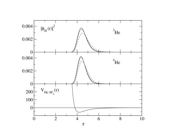
Figure 1: Dimer radial probability densities (³He-SF₆: upper panel; ⁴He-SF₆: middle panel); He-SF₆ interaction (lower panel). The probability densities correspond to the quantum numbers $\ell=0$ (solid line), $\ell=4$ (dashed line) and $\ell=8$ and 9 (dash-dotted line) for ³He and ⁴He, respectively. Distances in Å, potential in K and densities in Å^-3.

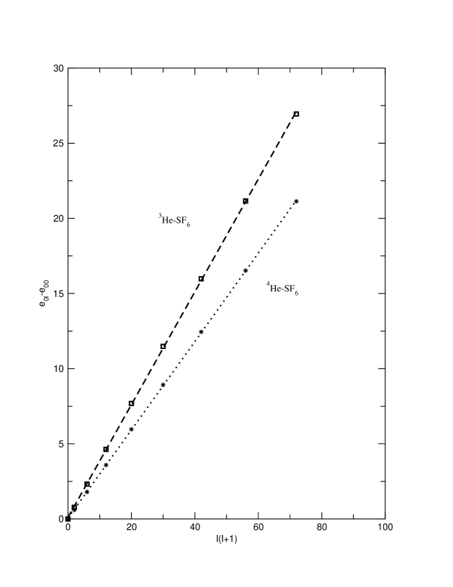
Figure 2: Differences $e_{0l}-e_{00}$ (in K) vs. $\ell(\ell+1)$ for the the He-SF₆ dimers. Squares correspond to the ³He-SF₆ results and stars to the ⁴He-SF₆ ones. The lines are linear fits to the numerical values.

The He-SF₆ interaction is displayed in Fig. 1. It is strongly repulsive at distances shorter than $\simeq 3.8$ Å, and attractive beyond. The attractive part is mostly concentrated in a narrow region around 4.2 Å, immediately after the repulsive core. This implies that the He atom locates relatively far away from the potential origin, so that the centrifugal term entering the Schrödinger equation can be considered as a perturbation. Two consequences can be deduced from this observation. First, the radial distributions are very peaked in the same narrow region, independently on the value of the angular momentum $\ell$, as it is shown in Fig. 1 for three states, corresponding to $\ell=0$ and 4 for both isotopes, and the nodeless bound states with the highest excitation energy, namely $\ell=8$ for ³He and 9 for ⁴He. The distributions are concentrated in the same region, and those corresponding to $\ell=0$ and 4 are barely distinguishible. Second, the excitation energies are closely proportional to $\ell(\ell+1)$, i.e. they follow a rotational pattern. Figure 2 depicts the differences $(e_{0\ell}-e_{00})$ in functions of $\ell(\ell+1)$ (squares for ³He-SF₆ and stars for ⁴He-SF₆), together with the linear fits to the energy differences. The slopes provide the $n=0$ rotational constants, $C_{0}^{(3,4)}$. From the the fits we obtain $C_{0}^{(3)}=0.376$ K and $C_{0}^{(4)}=0.294$ K, in good agreement with the rough estimate $\hbar^{2}/2m\langle R^{2}\rangle$, where $\langle R^{2}\rangle$ is the mean square Dopant-Helium distance. A similar behavior is found for the $n=1$ excited states, whose rotational constants are $C_{1}^{(3)}=0.194$ K and $C_{1}^{(4)}=0.179$ K. The ratio of the rotational constants of the dimers with either isotope are of course in the inverse ratio of masses. Notice that the larger mass of the ⁴He atom translates into a larger binding. Both the decrease of the kinetic energy and the increase of the attraction contribute to the increment of the binding energy for the ⁴He-SF₆ dimer. The stronger localization of the ⁴He atom is visualized by the peak of the radial probability density shown in Fig. 1, which is slightly higher for the ⁴He atom.

It is worth stressing that the observed rotational spectrum is a direct consequence of the shape of the He-SF₆ interaction, whose attractive well, having a depth of $\approx-57$ K, allows for twelve or fifteen bound states. Taking the lighter Ne as a dopant, we have found that only three bound states exist, being the depth of the attractive well $\approx-20$ K. Moreover, the binding energies are very small, and the probability distributions are extended over a large region.

III The He₂-SF₆ trimers: theory

In the limit of infinite mass of the dopant molecule, hence considered as a fixed center, the Hamiltonian of the He₂-SF₆ trimers is

$$H(1,2)=-\sum_{i=1}^{2}{\hbar^{2}\over 2m_{\alpha_{i}}}\nabla^{2}_{i}+\sum_{i=1}^{2}V_{\rm D-He}({\bf r}_{i})+V_{\rm He-He}({\bf r}_{12})\,$$ (3)

with $\alpha_{i}=3,4$. $V_{\rm D-He}({\bf r})$ and $V_{\rm He-He}({\bf r})$ are the dopant–helium and helium–helium interaction potentials, respectively. ${\bf r}_{i}$ is the coordinate of the $i$–th helium atom with respect to the central molecule and ${\bf r}_{12}$ is the helium–helium relative coordinate.

The ground and excited states properties of the trimers can be obtained either by an exact solution of the Schrödinger equation,

$$H(1,2)\,\Psi_{\gamma}^{T}(1,2)\,=\,E_{\gamma}\,\Psi_{\gamma}^{T}(1,2)\,$$ (4)

or by some approximate estimate of their wave functions. Here $\gamma$ labels the generic trimer state, whose wave function is $\Psi_{\gamma}^{T}(1,2)$.

The Schrödinger equation for clusters of ⁴He atoms may be exactly solved for the ground state by quantum Monte Carlo (QMC) methods.Chi92 ; Bar93 ; Lew97 Other approaches, as Variational Monte CarloPan86 ; Chi95 ; Gua01 (VMC) with Jastrow correlated wave functions or density functional theoriesStr87 ; Dal95 (DFT), provide a less accurate description of the clusters. However, they are generally more flexible than QMC.

The presence of more than two ³He atoms makes the exact solution of the Schrödinger equation much more difficult, because of the notorious sign problemsign associated to their fermionic nature. As a consequence, only DFT based studies of doped ³He clusters are available in literature.Bar97b ; Gar98 The most updated study of the ³He₂-SF₆ trimer has been done within the Hartree-Fock (HF) approximation, not considering the strong He-He correlations induced by $V_{\rm He-He}$.Jun01

In this Section we will first present a variational approach based on a Jastrow (J) correlated wave function. Then we will apply the Correlated Harmonical Hyperspherical (CHH) expansion methodCHH to further improve the description of the doped trimers.

III.1 Variational approach

The Jastrow correlated wave function of the trimer for the $\gamma$–state is given by:

$$\Psi_{\gamma}^{J}(1,2)\,=\,\Phi_{\gamma}(1,2)\,f_{J}(r_{12})\,$$ (5)

where $\Phi_{\gamma}(1,2)$ is an independent particle (IP) wave function of the two helium atoms in the dopant field having the same set, $\gamma$, of quantum numbers. The correlation function between the two atoms, $f_{J}(r)$, is assumed to depend only on the interatomic distance and takes into account the modification to the IP wave function mainly due to the He-He interaction. The optimal $f_{J}(r)$ is variationally fixed by minimizing the total energy of the state. $\Phi_{\gamma}(1,2)$ is built as an appropriate combination of the dimer He-SF₆ wave functions. For instance, using the $(LS)^{\pi}$ notation ($L$ being the IP orbital angular momentum, $S$ the total spin and $\pi$ the parity of the helium pair), the $(00)^{+}$ IP wave function for the ³He₂-SF₆ trimer is taken as:

$$\Phi_{(00)^{+}}(1,2)\,=\,\Xi_{0}(1,2)\,\phi_{1s}({\bf r}_{1})\phi_{1s}({\bf r}_{2})\,$$ (6)

where $\Xi_{0}(1,2)$ is the spin-singlet wave function of the ³He-³He pair and $\phi_{1s}({\bf r})$ is the $1s$ ($n$=0 and $\ell$=0) solution of the ³He-SF₆ dimer Schrödinger equation (1).

In an analogous way, the $(10)^{-}$ and $(11)^{-}$ IP wave functions are:

$$\Phi_{(10)^{-}}(1,2)\,=\,\Xi_{0}(1,2)\,{1\over{\sqrt{2}}}[\phi_{1s}({\bf r}_{1})\phi_{1p}({\bf r}_{2})+\phi_{1p}({\bf r}_{1})\phi_{1s}({\bf r}_{2})]\,$$ (7)

and

$$\Phi_{(11)^{-}}(1,2)\,=\,\Xi_{1}(1,2)\,{1\over{\sqrt{2}}}[\phi_{1s}({\bf r}_{1})\phi_{1p}({\bf r}_{2})-\phi_{1p}({\bf r}_{1})\phi_{1s}({\bf r}_{2})]\,$$ (8)

where $\Xi_{1}(1,2)$ is the spin-triplet pair wave function.

The total Hamiltonian (3) can be written as:

$$H(1,2)=h_{0}(1)+h_{0}(2)+V_{He-He}({\bf r}_{12})=H_{0}(1,2)+V_{He-He}({\bf r}_{12})\,$$ (9)

where $h_{0}$ is the Hamiltonian (2) of the dimer, and

$$H_{0}(1,2)\,\Phi_{\gamma}(1,2)\,=\,(e_{\gamma_{1}}+e_{\gamma_{2}})\,\Phi_{\gamma}(1,2)\,$$ (10)

where the two sets of dimer quantum numbers, $\gamma_{1}$ and $\gamma_{2}$, are those taken to build up the total $\gamma$-trimer state.

The total energy of the trimer in the $\gamma$-state is

$$E_{\gamma}={{\langle\Psi^{J}_{\gamma}|H(1,2)|\Psi^{J}_{\gamma}\rangle}\over{\langle\Psi^{J}_{\gamma}|\Psi^{J}_{\gamma}\rangle}}\,.$$ (11)

Since $[V_{D-He},f_{J}]=0$, the energy results to be:

$$E_{\gamma}=e_{\gamma_{1}}+e_{\gamma_{2}}+\sum_{i=1}^{2}{\hbar^{2}\over 2m_{\alpha_{i}}}{{\langle\Phi_{\gamma}|\nabla_{i}f_{J}(r_{12})\cdot\nabla_{i}f_{J}(r_{12})|\Phi_{\gamma}\rangle}\over{\langle\Psi^{J}_{\gamma}|\Psi^{J}_{\gamma}\rangle}}+{{\langle\Phi_{\gamma}|f_{J}(r_{12})V_{He-He}({\bf r}_{12})f_{J}(r_{12})|\Phi_{\gamma}\rangle}\over{\langle\Psi^{J}_{\gamma}|\Psi^{J}_{\gamma}\rangle}}\,.$$ (12)

This equation will be used to estimate the variational energy of the trimer and to optimize the choice of the correlation factor.

III.2 CHH approach

In order to implement the CHH method for a system of three atoms of masses $m_{i}$, in positions ${\bf r}_{i}$, it is convenient to introduce the three sets $({\bf x}_{i},{\bf y}_{i})$ of Jacobi coordinates:

$$\begin{array}[]{l}{\bf x}_{i}=\sqrt{\frac{m_{k}m_{j}}{m_{j}+m_{k}}}({\bf r}_{j}-{\bf r}_{k})\,,\\ {\bf y}_{i}=\sqrt{\frac{m_{i}(m_{j}+m_{k})}{m_{i}+m_{j}+m_{k}}}({\bf r}_{i}-\frac{m_{j}{\bf r}_{j}+m_{k}{\bf r}_{k}}{m_{j}+m_{k}})\,.\end{array}$$ (15)

In the fixed-center limit ($m_{3}=\infty$) the position ${\bf r}_{3}$ coincides with the molecular center of mass and, for two equal mass atoms ($m_{1}=m_{2}=m$), the Jacobi coordinates, after dividing by $m^{1/2}$, can be reduced to:

$$\left\{\begin{array}[]{l}{\bf x}_{1}={\bf r}_{2}\\ {\bf y}_{1}={\bf r}_{1}\end{array}\right.,\,\left\{\begin{array}[]{l}{\bf x}_{2}=-{\bf r}_{1}\\ {\bf y}_{2}={\bf r}_{2}\end{array}\right.,\,\left\{\begin{array}[]{l}{\bf x}_{3}=\sqrt{\frac{1}{2}}({\bf r}_{1}-{\bf r}_{2})\\ {\bf y}_{3}=-\sqrt{\frac{1}{2}}({\bf r}_{1}+{\bf r}_{2})\end{array}\right..$$ (16)

The total wave function, $\Psi_{(LS)^{\pi}}(1,2)$, can be expressed as a sum of three Faddeev-like amplitudes,CHH1 each of wich explicitely depends upon a different Jacobi set:

$$\Psi_{(LS)^{\pi}}(1,2)=\psi^{(1)}_{(LS)^{\pi}}({\bf x}_{1},{\bf y}_{1})+\psi^{(2)}_{(LS)^{\pi}}({\bf x}_{2},{\bf y}_{2})+\psi^{(3)}_{(LS)^{\pi}}({\bf x}_{3},{\bf y}_{3})\,.$$ (17)

The amplitudes are then expanded into channels, labelled by the partial angular momenta, $\ell_{x,i}$ and $\ell_{y,i}$, associated with ${\bf x}_{i}$ and ${\bf y}_{i}$, respectively:

$$\psi^{(i)}_{(LS)^{\pi}}({\bf x}_{i},{\bf y}_{i})=\Xi_{S}(1,2)\sum_{\ell_{x,i},\ell_{y,i}}\Phi^{(i)}_{\ell_{x,i},\ell_{y,i}}(x_{i},y_{i})[Y_{\ell_{x,i}}(\hat{x}_{i})Y_{\ell_{y,i}}(\hat{y}_{i})]_{LM}\,,$$ (18)

where $Y_{\ell}$ are ordinary spherical harmonics, and $\Phi^{(i)}_{\ell_{x,i},\ell_{y,i}}$ is a two-dimensional function depending upon the moduli of the Jacobi vectors. As a result, the parity of the state is given by $\ell_{x,i}+\ell_{y,i}$, even (odd) for positive (negative) parity.

Following Ref. bk2001, , each amplitude $\Phi^{(i)}_{\ell_{x,i},\ell_{y,i}}$ is expanded in terms of a correlated hyperspherical harmonics basis set. After introducing the hyperspherical coordinates, $(\rho,\phi_{i})$, associated with the Jacobi set:

$$\rho^{2} = x_{1}^{2}+y_{1}^{2}=x_{2}^{2}+y_{2}^{2}=x_{3}^{2}+y_{3}^{2}\,,$$ (19)

$$x_{i} = \rho\cos\phi_{i}\,,$$ (20)

$$y_{i} = \rho\sin\phi_{i}\,,$$ (21)

the CHH basis elements, having quantum numbers $(LS)^{\pi}$ and corresponding to the set of Jacobi coordinates labelled by $i$, are defined as follows:

$$|m,k,\ell_{x,i},\ell_{y,i};i\rangle = \Xi_{S}(1,2)F_{J}(r_{1},r_{2},r_{12})\rho^{\ell_{x,i}+\ell_{y,i}}L^{(5)}_{m}(z)\exp(-{z\over 2})$$ (22)

$$\times {}^{(2)}P^{\ell_{x,i},\ell_{y,i}}_{k}(\phi_{i})[Y_{\ell_{x,i}}({\hat{x}}_{i})Y_{\ell_{y,i}}({\hat{y}}_{i})]_{LM}\,,$$

where ${}^{(2)}P^{\ell_{x},\ell_{y}}_{k}(\phi)=N_{\ell_{x},\ell_{y},k}(\cos\phi)^{\ell_{x}}\,(\sin\phi)^{\ell_{y}}P^{\ell_{y}+1/2,\ell_{x}+1/2}_{k}(\cos(2\phi))$ is a normalized hypherspherical polynomial, $P^{\ell_{y}+1/2,\ell_{x}+1/2}_{k}$ is a Jacobi polynomial, $L^{(5)}_{m}$ are associated Laguerre polynomials, and $z=\beta\rho$, with $\beta$ a non-linear variational parameter.

The other ingredient in the CHH basis elements is the correlation factor, $F_{J}(r_{1},r_{2},r_{12})$. Due to the strongly repulsive core of the interatomic potentials, it is convenient to take $F_{J}$ as a product of pairwise Jastrow-like correlation functions,

$$F_{J}(r_{1},r_{2},r_{12})=g(r_{1})g(r_{2})f_{J}(r_{12})\,.$$ (23)

The correlation functions mainly describe the short-range behavior of the wave function as the two helium atoms are close to each other or to the dopant. The polynomial part of the CHH expansion is expected to reproduce the mid- and long-range configurations. Therefore, it is preferable to choose correlation functions which behave in the outer portion of the Hilbert space as smoothly as possible, in order to avoid potentially deleterious biasing of the polynomial expansion.

Suitable correlation functions to be used in (23) are obtained by solving the two-body Schrödinger equation:

$$\left(-\frac{\hbar^{2}}{2\mu}\nabla^{2}+V^{*}(r)+\lambda e^{-\xi r}\right)h(r)=0\,,$$ (24)

where $\mu$ is the reduced mass of the considered two-body system, and the pseudo-potential, $\lambda e^{-\xi r}$, is introduced to adjust the asymptotic behavior of the correlation function in such a way that $h(r\rightarrow\infty)\rightarrow 1$. The parameters $\xi$ and $\lambda$ are optimized for each of the different cases, SF₆-He, ⁴He-⁴He and ³He-³He. For the helium-dopant correlation ($h=g$), we take $\mu=m_{\rm He}$, and $V^{*}$ is a modified SF₆-He potential. In fact, in order to build a nodeless correlation function, it is necessary to reduce the attractive part of the helium-dopant interaction. The repulsive part, on the other hand, is kept unaltered. In the ⁴He-⁴He case ($h=f_{J}$, $\mu=m_{{}^{4}He}/2$), the correlation function has been obtained as in Ref. bk2001, . The ³He-³He pair does not support a bound state, so the correlation function has been obtained simply as the solution of the zero-energy Schrödinger equation ($V^{*}=V_{He-He}$ and $\lambda=0$ in Eq. 24).

In order to work with basis elements of defined symmetry under the permutation operator $\Pi_{12}$ (according to the Pauli principe) we take proper symmetric or antisymmetric combinations of the basis elements with $i=1$ and $2$:

$$|m,k,\ell_{x,1},\ell_{y,1};\nu\rangle=|m,k,\ell_{x,1},\ell_{y,1};1\rangle+(-1)^{q}|m,k,\ell_{x,1},\ell_{y,1};2\rangle\,,$$ (25)

where $\nu$ $(\equiv s,a)$ labels symmetric or antisymmetric states, respectively, and $q$=0, 1 is choosen according to the values of $\ell_{x}$ and $S$.

The expansion of the total wave function in terms of CHH states with well defined permutation symmetry results in:

$$\Psi_{(LS)^{\pi}}=\sum_{\ell_{x,1},\ell_{y,1}}\sum_{k_{a},m_{a}}A_{k_{a},m_{a}}|k_{a},m_{a},\ell_{x,1},\ell_{y,1};\nu\rangle+\sum_{\ell_{x,3},\ell_{y,3}}\sum_{k_{b},m_{b}}B_{k_{b},m_{b}}|k_{b},m_{b},\ell_{x,3},\ell_{y,3};3\rangle\,.$$ (26)

The sum over the partial angular momenta $\ell_{x},\ell_{y}$, although constrained by the values of the total angular momentum $L$, the parity and by symmetry considerations, runs over an infinite number of channels. However, in practice only the lower channels are included, since the higher the angular momentum the less the contribution to the wave function. Moreover, due to the presence of both the correlation factors $F_{J}$ and the amplitude expansion, an infinite number of channels is automatically included, though in a non-flexible way.

In the description of the $(LS)^{\pi}=(00)^{+},(10)^{-},(11)^{-}$ states for ³He₂-SF₆, we have retained only the lowest angular momentum channels, that is, $\ell_{x,1}=\ell_{y,1}=\ell_{x,3}=\ell_{y,3}=0$ for $(00)^{+}$, $\ell_{x,1}=\ell_{x,3}=0$ and $\ell_{y,1}=\ell_{y,3}=1$ for $(10)^{-}$, $\ell_{x,1}=\ell_{x,3}=1$ and $\ell_{y,1}=\ell_{y,3}=0$ for $(00)^{-}$. The CHH wave functions for these three states are:

$$\Psi_{(00)^{+}}(1,2)=\Xi_{0}(1,2)F_{J}e^{-z/2}\left\{\sum_{k_{a},m_{a}}A_{k_{a},m_{a}}L^{(5)}_{m_{a}}(z)P_{k_{a}}^{1/2,1/2}(\cos 2\phi_{1})\right.$$

$$+\left.\sum_{k_{b},m_{b}}B_{k_{b},m_{b}}L^{(5)}_{m_{b}}(z)P_{k_{b}}^{1/2,1/2}(\cos 2\phi_{3})\right\}\,,$$ (27)

$$\Psi_{(10)^{-}}(1,2)=\Xi_{0}(1,2)F_{J}e^{-z/2}\left\{\sum_{k_{a},m_{a}}A_{k_{a},m_{a}}L^{(5)}_{m_{a}}(z)\left[\rho\sin{\phi_{1}}P_{k_{a}}^{3/2,1/2}(\cos 2\phi_{1})Y^{M}_{1}(\hat{y}_{1})\right.\right.$$

$$+\rho\cos{\phi_{1}}\left.\left.P_{k_{a}}^{3/2,1/2}(-\cos 2\phi_{1})Y^{M}_{1}(\hat{x}_{1})\right]+\sum_{k_{b},m_{b}}B_{k_{b},m_{b}}L^{(5)}_{m_{b}}(z)\rho\sin{\phi_{3}}P_{k_{b}}^{3/2,1/2}(\cos 2\phi_{3})Y^{M}_{1}(\hat{y}_{3})\right\}\,,$$ (28)

$$\Psi_{(11)^{-}}(1,2)=\Xi_{1}(1,2)F_{J}e^{-z/2}\left\{\sum_{k_{a},m_{a}}A_{k_{a},m_{a}}L^{(5)}_{m_{a}}(z)\left[P_{k_{a}}^{1/2,3/2}(\cos 2\phi_{1})\rho\cos{\phi_{1}}Y^{M}_{1}(\hat{x}_{1})\right.\right.$$

$$-\rho\sin{\phi_{1}}\left.\left.P_{k_{a}}^{1/2,3/2}(-\cos 2\phi_{1})Y^{M}_{1}(\hat{y}_{1})\right]+\sum_{k_{b},m_{b}}B_{k_{b},m_{b}}L^{(5)}_{m_{b}}(z)\rho\cos{\phi_{3}}P_{k_{b}}^{1/2,3/2}(\cos 2\phi_{3})Y^{M}_{1}(\hat{x}_{3})\right\}\,,$$ (29)

where $k_{a}\geq 0$ and $k_{b}\geq 1$. However, only even values of $k_{a}$ are allowed in $\Psi_{(00)^{+}}$. In ⁴He₂-SF₆ we just study $\Psi_{(00)^{+}}$ and $\Psi_{(10)^{-}}$ states, since only $S=0$ combinations are possible.

In Eqs. (27–29) the linear coefficients, $\{A_{k_{a},m_{a}}\}$ and $\{B_{k_{b},m_{b}}\}$, are unknown quantities to be determined. The implementation of the variational principle for linear variational parameters leads to a generalized eigenvalues problem whose solutions, ${E_{i}}$, are upper bounds to the true energy eigenvalues of the three-body Schrödinger equation. It is possible to improve the estimates of the energies by including a larger number of polynomials and channels in the CHH basis. If $N$ is the dimension of the basis set, the estimates ${E_{i}^{N}}$ will monotonically converge from above to the exact eigenvalues as $N$ is increased. The pattern of convergence for the $(00)^{+}$ two lowest lying state of ³He₂-SF₆ is shown in Table 2. An optimum choice of the non-linear parameter $\beta$ has been adopted to improve the convergence rate.

IV Results

Table 3 collects the energies for the He₂-SF₆ trimers in the uncorrelated, Jastrow and CHH approaches. The correlation function is set equal to unity in the uncorrelated calculations, whereas it has been choosen of the McMillanMcMillan form,

$$f_{J}(r)=\exp\left[-{1\over 2}\left({{b\sigma}\over r}\right)^{5}\right]\,,$$ (30)

in the variational case. Here, $\sigma$=2.556 Å and $b$ is the only non-linear variational parameter. This type of correlation has been widely adopted in variational studies of liquid helium since it provides an excellent description of the short-range properties of the correlated wave function. In fact, it gives the exact short-range behavior for a 12–6 Lennard–Jones atom–atom interaction. The correlation operator adopted in the CHH expansion has been described in the previous section. In the CHH case we use different correlation functions since a non-linear parameter, $\beta$, is already present in the basis functions (see Eq. 22). Therefore, employing the McMillan form would imply a two non-linear parameters minimization. However, it has been checked that the use of the McMillan correlation in the CHH expansion produces binding energies within $0.01\%$ of those given in Table 3, showing that the converged results are to large extent independent of the correlation function, provided the short range behavior is adequately described. In Table 3, we also show the kinetic ($T$) and potential ($V$) contributions to the energy, separating the latter in its dopant-helium (D-He) and helium-helium (He-He) parts.

The uncorrelated trimers are unbound in all states, with the exception of the spatially antisymmetric (11)^- for ³He₂-SF₆. The orbital antisymmetry reduces the probability of configurations having the two ³He atoms close to each other. Hence, the contribution of the strong He-He repulsion at short distances is drastically suppressed. In Ref. Jun01, an expansion of the single-particle helium $s$- and $p$-orbitals in a finite set of gaussian basis functions centered at the dopant provided an energy of -31.36 K for the (11)^- state in ³He₂-SF₆. This energy is higher than our uncorrelated estimate, pointing to a lack of convergence in the Hartree-Fock result in that reference.

The introduction of the Jastrow correlation bounds all trimers, as it suppresses the short-range helium-helium repulsion. The L=0, positive parity states are the lowest lying ones, the other states having small excitation energies, lower than 1 K. The values of the variational parameter giving the minimum energies are also reported in the Table. The $b$-values for the spatially symmetric trimers are close to those found in the Jastrow correlated studies of bosonic liquid ⁴He. As in fermionic liquid ³He, $b$ is smaller for the spatially antisymmetric (11)^- state, since both the correlation and the Pauli principle concur in depleting the $V_{\rm He-He}(r)$ repulsion.

The converged CHH expansion provides slightly more binding (at most about -0.1 K) to the trimers. This fact is a strong indication of the high efficiency of the simple Jastrow correlated wave function in these systems. The kinetic and dopant-helium potential energies do not vary much in going from the uncorrelated to the variational and CHH estimates. The helium-helium potential energy is, instead, strongly dependent on the wave-function. For the uncorrelated cases the repulsive core is overwhelmingly dominant, except in the Pauli suppressed (11)^- state. The short-range structure of the correlated and CHH wave functions results in a slightly attractive value of $\langle V_{\rm He-He}\rangle$ (from -0.3 K to -1.6 K).

For the mixed ³He-⁴He-SF₆ trimer we give only the energies of the lowest lying (0)⁺ state. The extension of the CHH theory presented in Section III to this type of trimer is straightforward. All energies consistently sit in between the lighter ³He₂-SF₆ and the heavier ⁴He₂-SF₆ cases.

It is worth noticing that the strong supression of the mutual He-He repulsion due to the correlations translates into a total binding energy which is very close to the sum of the two dimer energies. The sum of the $\ell=0$ energies of Table 1 gives $-54.67$, $-61.13$ and $-57.90$ K, respectively, for the combinations ³He₂, ⁴He₂ and ³He-⁴He, which are very close to the binding energies of the trimer. The practical effect of the correlations is to reduce the He-He interaction to a small attraction of $\approx 0.1-0.2$ K. This result is very different from the findings of Ref. Jun01, , with total binding energies smaller than ours by roughly a factor of two.

We use a simple argument to estimate the accuracy of the infinite dopant mass approximation. From Table III we observe that, to a very good extent, the He₂-SF₆ trimer can be considered as the superposition of two independent He-SF₆ dimers. Accordingly, the $\alpha$–$\beta$–trimer corrected kinetic energy results $T^{(\alpha,\beta)}=T^{(\alpha,\beta)}_{M=\infty}[1+1/2(m_{\alpha}/M+m_{\beta}/M)]$. This correction corresponds to a modification of the total trimer energy less than $1\%$.

Structural properties of the trimers are shown in Table 4. We give the root-mean-square (rms) dopant-helium distance, $\sqrt{\langle R^{2}\rangle}$, the rms helium-helium distance, $\sqrt{\langle r^{2}_{12}\rangle}$, and the average value of the cosine between the two D-He radii, $\langle\cos(\theta_{12})\rangle$, in the three approaches. $\sqrt{\langle R^{2}\rangle}$ is not very sensitive to the introduction of the He-He correlation. For a given trimer, it assumes essentially the same values in the different states, reflecting the fact that the D-He wave functions, $\phi_{1s}$ and $\phi_{1p}$, are similar. Since the He-SF₆ interaction is the same for both helium isotopes, the smaller ³He mass would produce a larger kinetic energy than ⁴He. In order to minimize the energy, this tendency is partially compensated by a larger value of $\sqrt{\langle R^{2}_{{\rm D}-^{3}{\rm He}}\rangle}$ with respect to $\sqrt{\langle R^{2}_{{\rm D}-^{4}{\rm He}}\rangle}$. The He-He average distance increases in going form the uncorrelated to the variational and CHH cases in the spatially symmetric states, as a consequence of the intoduction of the correlation, which suppresses short-range He-He configurations. The effect is not very visible in the spatially antisymmetric state, (11)^-, being these configurations already largely inhibited by the Pauli principle. We even find a small decrease of $\sqrt{\langle r^{2}_{12}\rangle}$ in this state after solving the CHH equations. The values of the uncorrelated average He-He cosine, $\langle\cos(\theta_{12})\rangle$, are immediately understood in terms of the structure of $\Phi_{(LS)^{\pi}}(1,2)$. Correlations change these values, mostly in the spatially symmetric $S=0$ states. For instance, the average cosine corresponds to $\theta_{12}=0.39\,\pi$ in the uncorrelated $(10)^{-}$ state of the ³He₂-SF₆ trimer, and to $\theta_{12}=0.45(0.44)\,\pi$ for the Jastrow (CHH) case. The change for the spatially antisymmetric state, $(11)^{-}$, is much less evident.

The one-body helium densities (OBD),

$$\rho^{(1)}_{\gamma}({\bf r}_{1})={{\int d{\bf r}_{2}|\Psi_{\gamma}(1,2)|^{2}}\over{\int d{\bf r}_{1}\int d{\bf r}_{2}|\Psi_{\gamma}(1,2)|^{2}}}$$ (31)

normalized as

$$\int d{\bf r}_{1}\,\rho^{(1)}_{\gamma}({\bf r}_{1})\,=\,1\,,$$ (32)

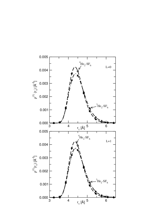
Figure 3: Helium densities in the $L$=0 (upper panel) and $L$=1 (lower panel) states of the He₂-SF₆ trimers. The symbols denote the uncorrelated densities, the lines stand for the CHH ones. In the upper panel the circles and the dashed line stand for ⁴He₂-SF₆ while the triangles and the dash-dotted line correspond to ³He₂-SF₆. The same notation is used for the L=1 ⁴He₂-SF₆ case in the lower panel. For the L=1 ³He₂-SF₆ trimer two states are reported, corresponding to S=0 (triangles and dotted line) and S=1 (stars and dash-dotted line). However, at the scale of the Figure they are hardly distinguishible.

are shown in Figure 3 for the $L$=0 and 1 states of the ³He₂-SF₆ and ⁴He₂-SF₆ trimers, obtained in the uncorrelated (symbols) and CHH (lines) approaches. The OBDs are very little affected by both the introduction of the He-He correlation and by the optimization of the D-He wave function. Actually, they are similar to the dimer radial probability densities shown in Fig. 1. As in the dimer case, the ⁴He atom is more localized than the ³He one because of its larger mass. For a given trimer, the OBDs do not appreciably depend on the $L$-values, since the $1s$ and $1p$ D-He wave functions are almost coincident.

Differences between the various approaches show up in the helium-helium two-body density (TBD), defined as:

$$\rho^{(2)}_{\gamma}({\bf r}_{1},{\bf r}_{2})={{|\Psi_{\gamma}(1,2)|^{2}}\over{\int d{\bf r}_{1}\int d{\bf r}_{2}|\Psi_{\gamma}(1,2)|^{2}}}\,\,.$$ (33)

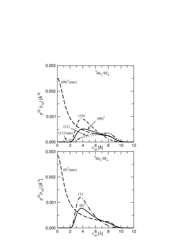
Figure 4: Helium-helium center-of-mass integrated two-body densities in the ³He₂-SF₆ (upper panel) and ⁴He₂-SF₆ (lower panel) trimers in the uncorrelated and CHH approaches. The uncorrelated (10)^- two body density for ³He₂-SF₆ is very close to the (00)⁺ one and it is not shown in the Figure. The same holds for the uncorrelated (1)^- TBD for ⁴He₂-SF₆.

In Figure 4 we display the center-of-mass integrated TBD,

$$\rho^{(2)}_{\gamma}({\bf r}_{12})=\int d{\bf R}_{12}\,\rho^{(2)}_{\gamma}({\bf r}_{1},{\bf r}_{2})$$ (34)

normalized as

$$\int d{\bf r}_{12}\,\rho^{(2)}_{\gamma}({\bf r}_{12})\,=\,1\,,$$ (35)

where ${\bf R}_{12}=(m_{1}{\bf r}_{1}+m_{2}{\bf r}_{2})/(m_{1}+m_{2})$ is the He-He center-of-mass coordinate and ${\bf r}_{12}={\bf r}_{1}-{\bf r}_{2}$ is the He-He distance. $\rho^{(2)}_{\gamma}({\bf r}_{12})$ gives the probability of the two helium atoms being at a distance $r_{12}$ apart.

The Pauli repulsion suppresses $\rho^{(2)}_{\gamma}({\bf r}_{12})$ in the uncorrelated (11)^- state of the ³He-SF₆ trimer at short He-He distances, in contrast with the uncorrelated (00)⁺ one. This behavior makes the former state bound and the latter unbound. We recall that the repulsive core of the He-He interaction is $R_{c}\sim\,2.5$ Å. The introduction of the He-He correlation depletes the TBD at small $r$-values in all the states, which result, as a consequence, all bound. In both trimers the helium atoms are more closely packed in the spatially symmetric, $L=1$ states, consistently with the values of $\sqrt{\langle r^{2}_{12}\rangle}$ shown in Table 4. As expected, the spatially antisymmetric (11)^- state is the most diffuse. The uncorrelated long-range structures of the TBDs remain essentialy untouched by the correlations.

We finally show in Figure 5 the TBD around the SF₆ molecule in the isosceles configurations, $\rho^{(2)}_{\gamma}(r_{1},r_{2}=r_{1},r_{12})$, for the uncorrelated and CHH (00)⁺, (10)^- and (11)^- states of ³He₂-SF₆. All of the TBDs vanish at low $r_{1}$ values because of the strong D-He repulsion. The isotropic distribution shown by the uncorrelated (00)⁺ TBD disappears after introducing the He-He correlation, which suppresses the density at low inter-helium distances. As already noticed in Fig. 4, the (11)^- TBD is the least affected by the correlations since it displays a short range He-He repulsion due to the Pauli principle.

V Summary and conclusions

The study of He₂-SF₆ trimers reveals the crucial role of the dopant heavy molecule in binding these systems. In fact, the SF₆ molecule acts as a fixed center of force in which the He atoms are moving. We have shown that the specific features of the SF₆-He interaction gives a rotational band in the excitation spectrum of the dimers. The different masses of the ³He and ⁴He explain in a qualitative way the particular features of each dimer. The solution of the dimer Schrödinger equation provides the single-particle wave functions needed to build the trial wave function to be used in the variational study of the trimers.

The ground state energies of the three isotopic trimers, namely ⁴He₂-SF₆, ³He₂-SF₆ and ⁴He-³He-SF₆, have been estimated employing a Jastrow correlated wave-function built up as the product of the dimer wave functions times a two-body correlation function of the McMillan type between the He atoms, having a single variational parameter. The accuracy of the variational approach has been tested against the Correlated Hyperspherical Harmonics expansion method. We have found that the variational results are in excellent agreement with the CHH ones at convergence.

The role of the Jastrow correlation is crucial in order to overcome the strong repulsion between the He atoms. Actually the uncorrelated variational approach does not bind the trimers, except the ³He₂-SF₆ one in the (11)^- configuration. The reason is that its wave function is spatially antisymmetric, and therefore the two ³He atoms are kept already apart by the Pauli repulsion. We stress that the preferred spatial configuration assumed by the two He atoms is such that they take advantage from the mutual attraction, suppressing, as much as possible, the short range repulsion. As a result, the optimal configuration is not a linear one, with the SF₆ molecule in the middle of the two He atoms. Instead, the He atoms are closer, and their position vectors with respect to the SF₆ molecule form an angle between $\simeq 70^{\rm o}$ and $\simeq 86^{\rm o}$, depending on the particular state. The practical effect of the correlations is that the binding energy of the trimer is slighlty larger than the sum of the binging energies of the corresponding dimers.

The He-He correlation does not particularly affect the the helium probability densities in the trimers, which are similar to those in the dimer. In contrast, the correlation is essential in inverting the energy hierarchy between the spatially symmetric and antisymmetric configurations. In fact, in the correlated ³He₂-SF₆ trimer the (00)⁺ state, symmetric in space with both He atoms in the $1s$ state and $S=0$, is more bound than the (11)^- state, antisymmetric in space with one atom in $1s$ and the other in the $1p$ state and $S=1$ (aligned spins). The uncorrelated approach does not even bind the (00)⁺ trimer, whereas the (11)^- one is still bound.

The good agreement between the variational and the CHH estimates for the trimers makes us confident that medium size He doped clusters can be accurately described by means of a correlated variational wave function. This trial wave function would be built up from the single-particle wave functions obtained after solving the dimer case, and from an appropriate Jastrow factor to properly take into account He-He correlations. In this respect, Variational Monte Carlo and Fermi Hypernetted Chain techniques seem to be the most likely candidates to microscopically address the study of medium-heavy doped helium nanodroplets.

	3He					4He
$\ell$	$e_{0\ell}$	$\langle V\rangle$	$\langle R\rangle$	$\sqrt{\langle R^{2}\rangle}$	$e_{1\ell}$	$e_{0\ell}$	$\langle V\rangle$	$\langle R\rangle$	$\sqrt{\langle R^{2}\rangle}$	$e_{1\ell}$
0	-27.336	-39.184	4.622	4.646	-1.940	-30.563	-41.509	4.549	4.568	-4.292
1	-26.561	-39.104	4.626	4.650	-1.541	-29.964	-41.459	4.552	4.571	-3.920
2	-25.016	-38.939	4.635	4.659	-0.775	-28.767	-41.355	4.557	4.577	-3.184
3	-22.707	-38.677	4.648	4.673		-26.976	-41.193	4.566	4.585	-2.105
4	-19.647	-38.298	4.667	4.693		-24.598	-40.963	4.577	4.597	-0.721
5	-15.854	-37.771	4.693	4.720		-21.641	-40.653	4.592	4.613
6	-11.354	-37.047	4.728	4.758		-18.117	-40.243	4.612	4.634
7	-6.183	-36.041	4.776	4.809		-14.040	-39.707	4.637	4.660
8	-0.394	-34.579	4.848	4.887		-9.431	-39.001	4.669	4.693
9						-4.318	-38.058	4.711	4.738

Table 1: Observables of the bound states of the He-SF₆ dimers. Energies are in K and distances in Å.

	$(00)^{+}$ ground state				$(00)^{+}$ first excited state
$n_{3}\backslash n_{1}$	1	2	3	4	1	2	3
0	-54.269	-54.652	-54.656	-54.656	-	-	-
1	-54.381	-54.743	-54.746	-54.746	-51.652	-51.674	-51.674
2	-54.397	-54.777	-54.780	-54.780	-52.384	-52.416	-52.416
3	-54.413	-54.789	-54.792	-54.792	-52.411	-52.439	-52.439
4	-54.414	-54.792	-54.795	-54.795	-52.425	-52.454	-52.454
5	-54.416	-54.793	-54.796	-54.796	-52.426	-52.455	-52.455
6	-54.416	-54.793	-54.796	-54.796	-52.427	-52.456	-52.456
7	-54.417	-54.793	-54.796	-54.797	-52.427	-52.457	-52.457
8	-54.417	-54.793	-54.796	-54.797	-52.427	-52.457	-52.457

Table 2: Convergence pattern of $E_{i}^{N}$ for the two lowest lying states of the $(00)^{+}$ band in ³He₂-SF₆ as a function of the numbers ($n_{1},n_{3}$) of Jacobi polynomials in the expansion (27) for the amplitude (1,2) and 3, respectively. The number of Laguerre polynomials is independently optimized for each case. The variational parameter $\beta$ is fixed to $1.59$ Å. Energies in K.

	3He-3He			4He-4He		3He-4He
	(00)+	(10)-	(11)-	(0)+	(1)-	(0)+
$b$	1.16	1.17	1.06	1.16	1.17	1.16
$E^{(unc)}$	837.18	1704.7	-33.378	931.84	1899.2	881.18
$E^{(var)}$	-54.746	-53.859	-54.078	-61.346	-60.783	-58.045
$E^{(CHH)}$	-54.797	-53.871	-54.161	-61.442	-60.843	-58.102
$T^{(unc)}$	23.696	24.390	24.390	21.892	22.440	22.794
$T^{(var)}$	23.936	24.948	24.389	22.074	22.869	23.004
$T^{(CHH)}$	24.301	25.587	24.553	22.668	23.713	23.528
$V^{(unc)}_{D-He}$	-78.368	-78.288	-78.288	-83.018	-82.967	-80.693
$V^{(var)}_{D-He}$	-78.045	-77.661	-78.213	-82.761	-82.469	-80.401
$V^{(CHH)}_{D-He}$	-78.392	-78.252	-78.402	-83.058	-82.988	-80.702
$V^{(unc)}_{He-He}$	891.85	1758.6	20.520	992.97	1959.7	939.08
$V^{(var)}_{He-He}$	-0.638	-1.146	-0.254	-0.660	-1.183	-0.649
$V^{(CHH)}_{He-He}$	-0.705	-1.206	-0.312	-1.052	-1.569	-0.908

Table 3: Total, kinetic and potential energies (in K) of the He₂-SF₆ trimers in the uncorrelated, variational and CHH approaches. $b$ is the adimensional parameter of the McMillan correlation function.

	3He-3He			4He-4He		3He-4He
	(00)+	(10)-	(11)-	(0)+	(1)-	(0)+
$\sqrt{\langle R^{2}\rangle}^{(unc)}$	4.646	4.648	4.648	4.568	4.570	4.646/4.568
$\sqrt{\langle R^{2}\rangle}^{(var)}$	4.655	4.665	4.650	4.576	4.584	4.656/4.575
$\sqrt{\langle R^{2}\rangle}^{(CHH)}$	4.645	4.645	4.653	4.568	4.569	4.646/4.567
$\sqrt{\langle r_{12}^{2}\rangle}^{(unc)}$	6.570	5.382	7.580	6.461	5.288	6.516
$\sqrt{\langle r_{12}^{2}\rangle}^{(var)}$	6.996	6.029	7.642	6.893	5.946	6.944
$\sqrt{\langle r_{12}^{2}\rangle}^{(CHH)}$	6.845	5.903	7.476	6.351	5.363	6.533
$\langle\cos(\theta_{12})\rangle^{(unc)}$	0	1/3	-1/3	0	1/3	0
$\langle\cos(\theta_{12})\rangle^{(var)}$	-0.133	0.163	-0.355	-0.138	0.157	-0.135
$\langle\cos(\theta_{12})\rangle^{(CHH)}$	-0.087	0.195	-0.298	0.033	0.260	-0.006

Table 4: Root mean square dopant-helium, $\sqrt{\langle R^{2}\rangle}$, and helium-helium, $\sqrt{\langle r_{12}^{2}\rangle}$, radii and average cosine between the two dopant-helium radii, $\langle\cos(\theta_{12}\rangle$ in the uncorrelated, variational and CHH approaches. In the first two rows of the last column, the first (second) value gives the D-³He (D-⁴He) rms radius. Distances in Å.

Figure 5: Helium-helium two-body densities in the isosceles configurations, $\rho^{(2)}_{\gamma}(r_{1},r_{2}=r_{1},r_{12})$, for the ³He₂-SF₆ trimer in the uncorrelated (00)⁺ ($a$), (10)^- ($c$) and (11)^- ($e$) states, and in the CHH (00)⁺ ($b$), (10)^- ($d$) and (11)^- ($f$) states. Distances in Å  and densities in Å^-6.

References

- (1) W. Schöllkopf and J.P. Toennies, Science 266, 1345 (1994).
- (2) W. Schöllkopf and J.P. Toennies, J. Chem. Phys. 104, 1155 (1996).
- (3) F. Luo, G.C. McBane, G. Kim, C.F. Giese, and W.R. Gentry, J. Chem. Phys. 98, 3564 (1993).
- (4) R.E. Grisenti, W. Schöllkopf, J.P. Toennies, G.C. Hegerfeldt, T. Köhler, and M. Stoll, Phys. Rev. Lett. 85, 2284 (2001).
- (5) A.R. Janzen and R.A. Aziz, J. Chem. Phys. 103, 9626 (1995).
- (6) M. Barranco, J. Navarro, and A. Poves, Phys. Rev. Lett. 78, 4729 (1997).
- (7) R. Guardiola and J. Navarro, Phys. Rev. Lett. 84, 1144 (2000).
- (8) R. Guardiola, Phys. Rev. B 62, 3416 (2000).
- (9) R.A. Aziz, F.R. McCourt and C.C.K. Wong, Mol, Phys. 61, 1487 (1987).
- (10) See e.g. J.P. Toennies in Microscopic Approaches to Quantum Liquids in Confined Geometries, E. Krotscheck, and J. Navarro Eds., World Scientific, Singapore, 2002.
- (11) Y. Kwong, P. Huang. M.H. Pavel, D. Blume, and K.B. Whaley, J. Chem. Phys. 113, 6469 (2000).
- (12) M. Barranco, M. Pi, S.M. Gatica, E.S. Hernández, and J. Navarro, Phys. Rev. B 56, 8997 (1997).
- (13) F. Garcias, Ll. Serra, M. Casas, and M. Barranco, J. Chem. Phys. 108, 9102 (1998).
- (14) P. Jungwirth and A.I. Krylov, J. Chem. Phys. 115, 10214 (2001).
- (15) R.T. Pack, E. Piper, G.A. Pfeffer, and J.P. Toennies, J. Chem. Phys. 80, 4940 (1984).
- (16) W.L. Taylor and J.J. Hurly, J. Chem. Phys. 98, 2291 (1993).
- (17) A. Kievsky, S. Rosati, and M. Viviani, Nucl. Phys. A551, 241 (1993).
-
(18)
A. Kievsky, S. Rosati, and M. Viviani,
Nucl. Phys. A577, 511 (1994);
M. Viviani, A. Kievsky, and S. Rosati, Few-Body Syst. 18, 25 (1995). - (19) S.A. Chin, and E. Krotscheck, Phys. Rev. B 45, 852 (1992).
- (20) R.N. Bartlett, and K.B. Whaley, Phys. Rev. A 47, 4082 (1993).
- (21) M. Lewerenz, J. Chem. Phys. 106, 4596 (1997).
- (22) V.R. Pandharipande, S.C. Pieper, and R.B. Wiringa, Phys. Rev. B 34, 4571 (1986).
- (23) S.A. Chin, and E. Krotscheck, Phys. Rev. B 52, 10405 (1995).
- (24) R. Guardiola, J. Navarro, and M. Portesi, Phys. Rev. B 63, 224519 (2001).
- (25) S. Stringari, and J. Treiner, J. Chem. Phys. 87, 5021 (1987).
- (26) F. Dalfovo, A. Lastri, L. Pricaupenko, S. Stringari, and J. Treiner, Phys. Rev. B 52, 1193 (1995).
- (27) See e.g. J. Boronat in Microscopic Approaches to Quantum Liquids in Confined Geometries, E. Krotscheck, and J. Navarro Eds., World Scientific, Singapore, 2002.
- (28) P. Barletta, and A. Kievsky, Phys. Rev. A64, 042514 (2001).
- (29) W.L. McMillan, Phys. Rev. 138, 442 (1965).