Focused X-shaped Pulses${}^{\>({\dagger})}$

Michel Zamboni-Rached,

D.M.O., Faculty of Electrical Engineering, UNICAMP, Campinas, SP, Brasil.

Amr M. Shaarawi$\;{{}^{*}}$

The Physics Department, The American University in Cairo, P.O.Box 2511, Cairo 11511, Egypt.

Erasmo Recami

Facoltà di Ingegneria, Università statale di Bergamo, Dalmine (BG), Italy;

and  INFN—Sezione di Milano, Milan, Italy.

Abstract  –   The space-time focusing of a (continuous) succession of localized X-shaped pulses is obtained by suitably integrating over their speed, i.e., over their axicon angle, thus generalizing a previous (discrete) approach. First, new Superluminal wave pulses are constructed, and then tailored in such a wave to get them temporally focused at a chosen spatial point, where the wavefield can reach for a short time very high intensities. Results of this kind may find applications in many fields, besides electromagnetism and optics, including acoustics, gravitation, and elementary particle physics.

PACS nos.:  41.20.Jb ;  03.50.De ;  03.30.+p ;  84.40.Az ;  42.82.Et ;  83.50.Vr ;   62.30.+d ;  43.60.+d ;   91.30.Fn ;   04.30.Nk ;   42.25.Bs ;  46.40.Cd ;  52.35.Lv  . OCIS codes:  320.5550 ;  320.5540 .

Keywords: Localized solutions to Maxwell equations; Superluminal waves; Bessel beams; Limited-diffraction pulses; Finite-energy waves; Electromagnetic wavelets; X-shaped waves; Electromagnetism; Microwaves; Optics; Special relativity; Localized acoustic waves; Seismic waves; Mechanical waves; Elementary particle physics; Gravitational waves

1. – Introduction

For many years it has been known that localized (non-diffractive) solutions exist to the wave equation[1]. Some localized wave solutions have peaks that travel at the speed of light, while others are endowed with subluminal or Superluminal velocities[2]. In more recent years, particular attention has been paid to the Superluminal[3-7] Localized Waves (SLW), that can have several applications such as high resolution imaging[8], secure communications, non-diffractive pulse propagation in material media[9-11], identification of buried objects[12], and so on.

The most characteristic SLWs resulted to be the so-called X-shaped solutions[13,3,4,6,14] (also named X-waves, in brief) whose structure and behavior are by now well understood, and experimentally reproduced[15-18]. Even their propagation along waveguides has been investigated[19].  In addition, their finite energy versions, with arbitrary frequencies and adjustable bandwidths[6,10,20], have been also constructed. Moreover, several investigations about constructing and generating approximate X-shaped waves from finite apertures[21,22] have been carried on.

In a recent paper by Shaarawi et al.[23], appeared in this Journal, it has been introduced a space-time focusing technique (called “Temporal focusing”), that had recourse to superpositions of localized X-waves traveling with different velocities. The various pulses were designed to reach a given spatial point $z=z_{\rm f}$ at the same time $t=t_{\rm f}$. In the mentioned work[23], the resulting composite X-shaped wave was synthesized as a discrete sum of individual X-waves. In the present paper we generalize that focusing scheme, by going on, in particular, to a continuous superposition of individual X-waves, i.e., to integrals (instead of discrete sums). We are moreover going to show how one can in general use any known Superluminal solution, to obtain from it a large number of analytic expressions for space-time focused waves, endowed with a very strong intensity peak at the desired location. Finally, we shall consider the case of the excitation of such pulses from finite-size apertures. At variance with the source-free case, the range over which the aperture-generated pulses can be focused is limited by the field depth of the single X-wave components.

2. – The Discrete Space-time Focusing Method

Let us first summarize the “temporal focusing” scheme developed in Ref.[23]. Since the velocity of the X-shaped waves depends on their apex angle $\theta$ (also known as the axicon angle), in the previous paper the space-time focusing was achieved by superimposing a discrete number of X-waves, characterized by different $\theta$ values. In this work, we’ll go on to more efficient superpositions for varying velocities $V$, related to $\theta$ through the known[3,4] relation $V=c/\cos\theta$. It will be shown in Section 3 that this enhanced focusing scheme has the advantage of yielding analytic (closed-form) expressions for the spatio-temporally focused pulses.

Consider an axially symmetric Superluminal wave pulse $\psi(\rho,z-Vt)$ in a dispersionless media, where $V>c$ is the pulse velocity and $(\rho,\phi,z)$ are the cylindrical co-ordinates. Pulses like these can be obtained by a superposition of Bessel beams[3,4,24], viz.,

$$\psi(\rho,z-Vt)\;=\;\int_{-\infty}^{\infty}\,S(\omega)\,J_{0}\left(\frac{\omega}{c}\,\sin\theta\,\rho\right)\,e^{i\frac{\omega}{c}\,\cos\theta\,(z-\frac{c}{\cos\theta}\,t)}{\rm d}\omega$$ (1)

where $\theta$ is the Bessel beam axicon angle, with $V=c/\cos\theta$, and $S(\omega)$ is the frequency spectrum. The center of such pulses is localized at $z=Vt$: Many solutions of this kind, as well as their finite energy version, can be found in Refs.[20,6].

Suppose that we have now $N$ waves of the type $\psi_{n}(\rho,z-V_{n}(t-t_{n}))$, with different velocities, $c<V_{1}<V_{2}<..<V_{N}$, and emitted at (different) times $t_{n}$; quantities $t_{n}$ being constants, while $n$=1,2,…$N$.  The center of each pulse is localized at

$$z\;=\;V_{n}\,(t-t_{n})$$ (2)

To obtain a highly focused wave, we need all wave components $\psi(\rho,z-Vt)$ to reach the given point, $z=z_{\rm f}$, at the same time $t=t_{\rm f}$. On choosing $t_{1}=0$ for the slowest pulse $\psi_{1}$, it is easily seen that the peak of this pulse reaches the point $z=z_{\rm f}$ at the time

$$t_{\rm f}\;=\;\frac{z_{\rm f}}{V_{1}}$$ (3)

Combining Eqs.(2) and (3), we obtain that for each $\psi_{n}$ the instant of emission $t_{n}$ must be

$$t_{n}\;=\;\left(\frac{1}{V_{1}}-\frac{1}{V_{n}}\right)z_{\rm f}$$ (4)

Therefore, a solution of the type

$$\Psi(\rho,z,t)\;=\;\sum_{n=1}^{N}A_{n}\psi_{n}(\rho,z-V_{n}(t-t_{n}))\ ,$$ (5)

where $A_{n}$ are constants, will represent a set of $N$ (initially separated) Superluminal waves, which just reach the position $z=z_{\rm f}$ at the same time $t=t_{\rm f}=z_{\rm f}/V_{1}$.

The scheme described above was essentially developed in Ref.[23] by using discrete X-waves: We have just replaced summations over $\theta$ with summations over $V$.  In the remaining part of this work, we propose a generalization of that idea, which can yield new classes of exact Superluminal solutions, besides providing enhanced focusing effects.

2.1 – The new space-time focusing scheme

In this Section, we extend the previous “temporal focusing” approach[23] by considering a continuous superposition, namely, by integrating over the velocity (instead of a discrete sum over the angle $\theta$).

Combining Eqs.(4) and (5), and going on to the integration over $V$, one gets

$$\Psi(\rho,z,t)\;=\;\int_{V_{\rm min}}^{V_{\rm max}}\,{\rm d}V\,A(V)\,\psi\left(\rho,z-V\left(t-\left(\frac{1}{V_{\rm min}}-\frac{1}{V}\right)z_{\rm f}\right)\right)\ ,$$ (6)

where $V$ is the velocity of the wave $\psi$ in Eq.(1). In the integration, $V$ is considered as a continuous variable in the interval $[V_{\rm min},V_{\rm max}]$. In Eq.(6), $A(V)$ is the velocity-distribution function that specifies the contribution of each wave component (with velocity $V$) to the integration. The resulting wave $\Psi(\rho,z,t)$ can have a more or less strong amplitude peak at $z=z_{\rm f}$, at time $t_{\rm f}=z_{\rm f}/V_{\rm min}$, depending on $A(V)$ and on the difference $V_{\rm max}-V_{\rm min}$.  Let us notice that also the resulting wavefield will propagate with a Superluminal velocity, depending on $A(V)$ too. In the cases when $A(V)$ can be actually considered a distribution function, namely, when $A(V)>0\,\,,\,\,\,\forall\ V$, and $\int_{V_{\rm min}}^{V_{\rm max}}\,{\rm d}V\,A(V)<\infty$, we can heuristically expect that the mean velocity $\overline{V}$ of the field (6) will be

$$\overline{V}\approx\displaystyle{\frac{\int_{V_{\rm min}}^{V_{\rm max}}\,A(V)\,V\,{\rm d}V}{\int_{V_{\rm min}}^{V_{\rm max}}\,A(V)\,{\rm d}V}}>c\ .$$ (7)

In the cases when the velocity-distribution function is well concentrated around a certain velocity value, one can expect the wave (6) to increase its magnitude and spatial localization while propagating. Finally, the pulse peak acquires its maximum amplitude and localization (at the chosen point $z=z_{\rm f}$, and at time $t=z_{\rm f}/V_{\rm min}$, as we know). Afterwards, the wave suffers a progressive spreading, and a decreasing of its amplitude.

3. – Enhanced Focusing Effects by Using Ordinary X-Waves

Here, we present a specific example by integrating, in Eq.(6), over the standard, ordinary[3,4] X-waves:

$$X(\rho,z-Vt)\;=\;\displaystyle{\frac{V}{\sqrt{(aV-i\,(z-Vt))^{2}+\left(\frac{V^{2}}{c^{2}}-1\right)\rho^{2}}}}\ .$$ (8)

The “classical” solution (8) can be obtained[3,6,4] by substituting the spectrum  $S(\omega)=\Omega(\omega)\;{\rm exp}(-a\,\omega)$  into Eq.(1), where $a$ is a constant that defines the bandwidth, $\Delta\omega=1/a$, and $\Omega(\omega)$ is the step-function. When using the zeroth-order X-waves above, however, the largest spectral amplitudes are obtained for low frequencies. For this reason, one may expect that the solutions considered below will be suitable mainly for low frequency applications.

Let us choose, then, the function $\psi$ in the integrand of Eq.(6) to be $\psi(\rho,z,t)\equiv X(\rho,z-V(t-(1/V_{\rm min}-1/V)z_{\rm f}))$, viz.,

$$\psi(\rho,z,t)\equiv X\;=\;\displaystyle{\frac{V}{\sqrt{\left[aV-i\left(z-V\left(t-\left(\frac{1}{V_{\rm min}}-\frac{1}{V}\right)z_{\rm f}\right)\right)\right]^{2}+\left(\frac{V^{2}}{c^{2}}-1\right)\rho^{2}}}}$$ (9)

After some manipulations, one obtains the analytic integral solution

$$\Psi(\rho,z,t)\;=\;\int_{V_{\rm min}}^{V_{\rm max}}\,\displaystyle{\frac{V\,A(V)}{\sqrt{PV^{2}+QV+R}}}{\rm d}V$$ (10)

with

$$\begin{array}[]{l}P\;=\;\left[\left(a+i\left(t-\frac{z_{\rm f}}{V_{\rm min}}\right)\right)^{2}+\frac{\rho^{2}}{c^{2}}\right]\\ \\ Q\;=\;2\left(t-\frac{z_{\rm f}}{V_{\rm min}}-ai\right)(z-z_{\rm f})\\ \\ R\;=\;\left[-(z-z_{\rm f})^{2}-\rho^{2}\right]\end{array}$$ (11)

3.1 – Some examples

In what follows, we illustrate the behavior of our new spatio-temporally focused pulses, by taking into consideration four different velocity distributions $A(V)$.

First case:

Let us consider our “integral solution” (10) with

$$A(V)\;=\;1\ .$$ (12)

In this case, the contribution of the X-waves is the same for all velocities in the allowed range $[V_{\rm min},V_{\rm max}]$, and Eq.(10) yields

$$\Psi(\rho,z,t)\;=\;\int_{V_{\rm min}}^{V_{\rm max}}\,\displaystyle{\frac{V}{\sqrt{PV^{2}+QV+R}}}{\rm d}V\ .$$ (13)

On using identity 2.264.2 of Ref.[25], we get the particular solution

$$\begin{array}[]{clcr}\Psi(\rho,z,t)\!\!&=\displaystyle{\frac{\sqrt{PV_{\rm max}^{2}+QV_{\rm max}+R}-\sqrt{PV_{\rm min}^{2}+QV_{\rm min}+R}}{P}}\\ \\ &\;\;\;\displaystyle{+\frac{Q}{2P^{3/2}}\,{\rm ln}\left(\frac{2\,\sqrt{P(PV_{\rm min}^{2}+QV_{\rm min}+R)}+2PV_{\rm min}+Q}{2\,\sqrt{P(PV_{\rm max}^{2}+QV_{\rm max}+R)}+2PV_{\rm max}+Q}\right)}\ ,\end{array}$$ (14)

where $P$, $Q$ and $R$ are given in Eq.(11). A 3-dimensional (3-D) plot of this function is provided in Fig.1; where we have chosen $a=10^{-12}$ s,  $V_{\rm min}=1.001\;c$,  $V_{\rm max}=1.005\;c$ and $z_{\rm f}=200\;$cm. It can be seen that this solution exhibits a rather evident space-time focusing. An initially spread-out pulse (shown for $t=0$) becomes highly localized at $t=t_{\rm f}=z_{\rm f}/V_{\rm min}=6.66\;$ns, the pulse peak amplitude at $z_{\rm f}$ being $40.82$ times greater than the initial one. In addition, at the focusing time $t_{\rm f}$ the field is much more localized than at any other times. The velocity of this pulse is approximately $\overline{V}=1.003\;c$.

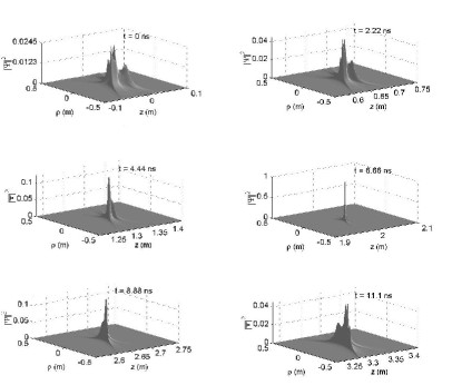
Figure 1:

Second case:

In this case we choose

$$A(V)\;=\;\frac{1}{V}$$ (15)

and Eq.(10) gives

$$\Psi(\rho,z,t)\;=\;\int_{V_{\rm min}}^{V_{\rm max}}\,\displaystyle{\frac{1}{\sqrt{PV^{2}+QV+R}}}{\rm d}V\ .$$ (16)

On using the identity 2.261 in Ref.[25], we obtain the new particular solution

$$\Psi(\rho,z,t)\;=\;\displaystyle{\frac{1}{\sqrt{P}}\,{\rm ln}\left(\frac{2\,\sqrt{P(PV_{\rm max}^{2}+QV_{\rm max}+R)}+2PV_{\rm max}+Q}{2\,\sqrt{P(PV_{\rm min}^{2}+QV_{\rm min}+R)}+2PV_{\rm min}+Q}\right)}\ .$$ (17)

Third case:

On substituting the velocity-distribution function

$$A(V)\;=\;\frac{1}{V^{2}}$$ (18)

into Eq.(10), one gets

$$\Psi(\rho,z,t)\;=\;\int_{V_{\rm min}}^{V_{\rm max}}\,\displaystyle{\frac{1}{V\,\sqrt{PV^{2}+QV+R}}}{\rm d}V$$ (19)

Because of identity 2.269.1 in Ref.[25], the above integration forwards the further particular solution

$$\Psi(\rho,z,t)\;=\;\displaystyle{\frac{1}{\sqrt{R}}\;{\rm ln}\left(\frac{V_{\rm max}(2R+QV_{\rm min}+2\sqrt{R(PV_{\rm min}^{2}+QV_{\rm min}+R)})}{V_{\rm min}(2R+QV_{\rm max}+2\sqrt{R(PV_{\rm max}^{2}+QV_{\rm max}+R)})}\right)}\ .$$ (20)

Fourth case:

With the velocity-distribution function given by

$$A(V)\;=\;\frac{1}{V^{3}}$$ (21)

we have from Eq.(10):

$$\Psi(\rho,z,t)\;=\;\int_{V_{\rm min}}^{V_{\rm max}}\,\displaystyle{\frac{1}{V^{2}\,\sqrt{PV^{2}+QV+R}}}{\rm d}V\ .$$ (22)

On using the identity 2.269.2 of Ref.[25], we get the last particular solution

$$\begin{array}[]{clcr}\Psi(\rho,z,t)\!\!&=\displaystyle{\frac{\sqrt{PV_{\rm min}^{2}+QV_{\rm min}+R}}{RV_{\rm min}}-\frac{\sqrt{PV_{\rm max}^{2}+QV_{\rm max}+R}}{RV_{\rm max}}}\\ \\ &\;\;\;\displaystyle{+\;\frac{Q}{2R^{3/2}}\;{\rm ln}\left(\frac{V_{\rm min}(2\,\sqrt{R(PV_{\rm max}^{2}+QV_{\rm max}+R)}+2R+QV_{\rm max})}{V_{\rm max}(2\,\sqrt{R(PV_{\rm min}^{2}+QV_{\rm min}+R)}+2R+QV_{\rm min})}\right)}\ .\end{array}$$ (23)

4. – Enhanced Space-time Focusing by Using Higher-Order X-Waves of Arbitrary Frequencies and Adjustable Bandwidths

The scheme presented in the preceding Section (confined to zeroth-order X-waves) can be extended to higher-order X-waves. Namely, one can use in the integrand of Eq.(6) the various time-derivatives of the ordinary X-waves, which have been shown[26] to constitute an infinite set of generalized X-wave solutions. This procedure will provide us with spatio-temporally focused Superluminal pulses that can have any arbitrary frequencies and adjustable bandwidths[6,10]. It has been also shown[26,7,10,6] that time derivatives of the X-waves can be constructed by substituting into Eq.(1) the frequency spectrum $S(\omega)=\Omega(\omega)\;\omega^{m}\,\exp(-a\,\omega)$, with $m$ an integer. A more general approach for obtaining infinite series of X-shaped solutions through suitable differentiations of the ordinary X-wave can be found in Ref.[6]; whilst more details about the properties of the frequency-spectra, which allows for closed-form solutions, can be found in the mentioned Refs.[10,7,6].

Namely: by using appropriate values for the parameters $m$ and $a$, it is possible to shift the central frequency, $\omega_{\rm c}$, and adjust the bandwidth, $\Delta\omega$, to any desired values[6,7,10]. The relationships among $\omega_{\rm c}$, $\Delta\omega$, $a$ and $m$ are

$$\left\{\begin{array}[]{l}\displaystyle{\omega_{\rm c}\;=\;\frac{m}{a}}\\ \\ m\;=\;\displaystyle{\frac{1}{\pm\frac{\Delta\omega_{\pm}}{\omega_{\rm c}}-{\rm ln}\left[1\pm\frac{\Delta\omega_{\pm}}{\omega_{\rm c}}\right]}}\end{array}\right.\ ,$$ (24)

where[7,10] $\Delta\omega_{+}$ ($>0$) is the bandwidth to the right, and $\Delta\omega_{-}$ ($>0$) is the bandwidth to the left of $\omega_{\rm c}$;  so that  $\Delta\omega=\Delta\omega_{+}+\Delta\omega_{-}$.

It is easy to show that[6,7,10]

$$\begin{array}[]{clcr}X^{(m)}(\rho,z-Vt)\!\!&\displaystyle{\equiv\int_{0}^{\infty}\,\omega^{m}\,e^{-a\,\omega}\,J_{0}\left(\frac{\omega}{c}\,\sin\theta\,\rho\right)\,e^{i\frac{\omega}{c}\,\cos\theta\,(z-\frac{c}{\cos\theta}\,t)}}{\rm d}\omega\\ \\ \!\!&\displaystyle{=i^{m}\,\frac{\partial^{m}X}{\partial t^{m}}}\ ,\end{array}$$ (25)

Let us now choose the function $\psi$ in the integrand of Eq.(6) to be  $\psi(\rho,z,t)\equiv i^{m}\,X^{(m)}(\rho,z-V(t-(1/V_{\rm min}-1/V)z_{\rm f}))$;  equation (6), then, yields the new (analytic) integral solution

$$\Psi(\rho,z,t)\;=\;\displaystyle i^{m}\frac{\partial^{m}}{\partial t^{m}}\int_{V_{\rm min}}^{V_{\rm max}}\,\displaystyle{\frac{V\,A(V)}{\sqrt{PV^{2}+QV+R}}}{\rm d}V\ ,$$ (26)

with $P$, $Q$ and $R$ given by Eq.(11).

Next, let us consider the cases of four different velocity-spectra, similar to the ones used in subsection 3.1.

4.1 – Some examples

First case:

Consider the integration in Eq.(26) with

$$A(V)\;=\;1\ .$$ (27)

On using the result in our previous Eq.(14), we find the particular solution

$$\begin{array}[]{clcr}\Psi(\rho,z,t)\!\!&=\displaystyle{i^{m}\,\frac{\partial^{m}}{\partial t^{m}}\left[\frac{\sqrt{PV_{\rm max}^{2}+QV_{\rm max}+R}-\sqrt{PV_{\rm min}^{2}+QV_{\rm min}+R}}{P}\right.}\\ \\ &\;\;\;\left.\displaystyle{+\;\frac{Q}{2P^{3/2}}\;{\rm ln}\left(\frac{2\,\sqrt{P(PV_{\rm min}^{2}+QV_{\rm min}+R)}+2PV_{\rm min}+Q}{2\,\sqrt{P(PV_{\rm max}^{2}+QV_{\rm max}+R)}+2PV_{\rm max}+Q}\right)}\right]\ .\end{array}$$ (28)

Second case:

Let us substitute

$$A(V)\;=\;\frac{1}{V}$$ (29)

into Eq.(26). On using the result in Eq.(17), one finds the new particular solution

$$\Psi(\rho,z,t)\;=\;i^{m}\,\frac{\partial^{m}}{\partial t^{m}}\left[\displaystyle{\frac{1}{\sqrt{P}}\;{\rm ln}\left(\frac{2\,\sqrt{P(PV_{\rm max}^{2}+QV_{\rm max}+R)}+2PV_{\rm max}+Q}{2\,\sqrt{P(PV_{\rm min}^{2}+QV_{\rm min}+R)}+2PV_{\rm min}+Q}\right)}\right]\ .$$ (30)

Third case:

On considering the velocity spectrum

$$A(V)\;=\;\frac{1}{V^{2}}$$ (31)

we obtain, after combining Eqs.(26) and (20), the further particular solution

$$\Psi(\rho,z,t)\;=\;i^{m}\,\frac{\partial^{m}}{\partial t^{m}}\left[\displaystyle{\frac{1}{\sqrt{R}}\;{\rm ln}\left(\frac{V_{\rm max}(2R+QV_{\rm min}+2\sqrt{R(PV_{\rm min}^{2}+QV_{\rm min}+R)})}{V_{\rm min}(2R+QV_{\rm max}+2\sqrt{R(PV_{\rm max}^{2}+QV_{\rm max}+R)})}\right)}\right]\ .$$ (32)

The plots in Fig.2 show that this solution implies a great space-time focusing effect. On using $m=1$,   $a=10^{-12}$ s,  $V_{\rm min}=1.001\;c$,  $V_{\rm max}=1.005\;c$, and $z_{\rm f}=200\;$cm, the peak amplitude at $z=z_{\rm f}$ results to be $1000$ times larger than the initial one, while, at the focusing time $t_{\rm f}=6.66$ns the field is much more localized than at any other times. The velocity of this pulse is approximately $\overline{V}=1.0029\;c$.

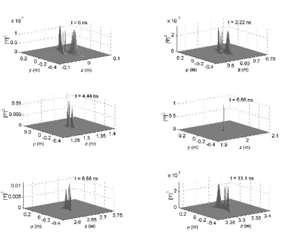
Figure 2:

Fourth case:

On substituting the velocity spectrum

$$A(V)\;=\;\frac{1}{V^{3}}$$ (33)

into Eqs.(26) and using the result (23), we get the last particular solution

$$\begin{array}[]{clcr}\Psi(\rho,z,t)\!\!&=\displaystyle{i^{m}\,\frac{\partial^{m}}{\partial t^{m}}}\left[\displaystyle{\frac{\sqrt{PV_{\rm min}^{2}+QV_{\rm min}+R}}{RV_{\rm min}}-\frac{\sqrt{PV_{\rm max}^{2}+QV_{\rm max}+R}}{RV_{\rm max}}}\right.\\ \\ &\;\;\;\left.\displaystyle{+\;\frac{Q}{2R^{3/2}}\;{\rm ln}\left(\frac{V_{\rm min}(2\,\sqrt{R(PV_{\rm max}^{2}+QV_{\rm max}+R)}+2R+QV_{\rm max})}{V_{\rm max}(2\,\sqrt{R(PV_{\rm min}^{2}+QV_{\rm min}+R)}+2R+QV_{\rm min})}\right)}\right]\ .\end{array}$$ (34)

5. – A More General Formulation

The results presented in the preceding Sections demonstrate that in Eq.(6) one can utilize any kind of Superluminal pulses towards the goal of producing large space-time focusing effects. A further generalization of our focusing scheme is introduced in the present Section.

Let us recall that a Superluminal wave with axial symmetry can be rewritten[6] as a superposition of Bessel beams expressed in terms of $V$ (instead of $\theta$):

$$\psi(\rho,z-Vt)\;=\;\displaystyle{\int_{-\infty}^{\infty}\,S(\omega)\,J_{0}\left(\frac{\omega}{V}\,\rho\,\sqrt{\left(\frac{V^{2}}{c^{2}}-1\right)}\,\,\right)\,e^{i\,\frac{\omega}{V}(z-Vt)}\,{\rm d}\omega}\ ,$$ (35)

where $J_{0}$ is the zeroth-order Bessel function and $S(\omega)$ is the frequency spectrum of the pulse $\psi(\rho,z-Vt)$. Now, by using the focusing method represented by our Eq.(6), one gets

$$\begin{array}[]{clcr}\Psi(\rho,z,t)=\displaystyle{\int_{V_{\rm min}}^{V_{\rm max}}{\rm d}V\,A(V)}&\displaystyle{\int_{-\infty}^{\infty}\,S(\omega)\,J_{0}\left(\frac{\omega}{V}\rho\sqrt{\left(\frac{V^{2}}{c^{2}}-1\right)}\,\right)}\\ \\ &\displaystyle{\times\,\exp\left[i\frac{\omega}{V}\,\{z-V\,[t-\,(\frac{1}{V_{\rm min}}-\frac{1}{V}\,)z_{\rm f}\,]\,\}\right]{\rm d}\omega}\;,\end{array}$$ (36)

which can be rewritten as

$$\Psi(\rho,z,t)=\displaystyle{\int_{V_{\rm min}}^{V_{\rm max}}{\rm d}V\,\int_{-\infty}^{\infty}B(\omega,V)\,J_{0}\left(\frac{\omega}{V}\rho\sqrt{\left(\frac{V^{2}}{c^{2}}-1\right)}\,\right)e^{i\frac{\omega}{V}(z-Vt)}e^{i\omega\left(\frac{1}{V_{\rm min}}-\frac{1}{V}\right)z_{\rm f}}\,{\rm d}\omega}\;.$$ (37)

From Eq.(37) it can be inferred that also the frequency-velocity weight functions of the form

$$\overline{S}(\omega,V)\,\equiv\,B(\omega,V)\,e^{i\,\omega\left(\frac{1}{V_{\rm min}}-\frac{1}{V}\right)z_{\rm f}}$$ (38)

are able to produce spatio-temporally focused pulses that propagate, once more, at Superluminal speeds. Such pulses can be considered as a continuous superposition of Bessel Beams of different frequencies and different velocities. Moreover, each Bessel beam, endowed with velocity $V$ and angular frequency $\omega$, possesses also a different phase with respect to the others, given by  ${\rm exp}(i\,\omega(1/V_{\rm min}-1/V)z_{\rm f}$.  In other words, the frequency-velocity spectra, generators of focused Superluminal pulses, determine not only the amplitudes of each Bessel beam in the superposition, but also the relative phases among them.  Along similar lines, Mugnai et al.[27] demonstrated that one can generate beams with a very hight optical resolving power by a superposition of Bessel beams with suitably chosen relative phase-delays. This was achieved by the use of a paraffin torus in each one of the coronae adopted for producing the various Bessel beams, the required phase delays being determined by the paraffin.  In a sense, the superpositions introduced in this work appear to reveal that an analogous phenomenon holds in the case of pulses too.

6. – Focused Pulses Generated from Finite Apertures

In the preceding Sections, we have demonstrated the effectiveness of our space-time focusing scheme in the case of source-free (composite) X-wave pulses. The analysis presented in Section 5 can be actually regarded as a powerful tool, that may be used to tailor an initially spread pulse, with the aim of focusing it at a pre-chosen point in space-time. The situation becomes more involved, however, when such a tailored pulse is generated from an aperture having a finite radius: In fact, the X-wave components having different velocities are characterized by different diffraction-free lengths (or “field depths”). More specifically,  $z_{\rm d}=D/(2\sqrt{\left(V/c\right)^{2}-1})$,  where $\,D\,$ is the diameter of the circular aperture.

To appreciate the effect of the finite size of the aperture on the space-time focusing scheme, we calculate the field radiated by a finite aperture using the Rayleigh-Sommerfeld (II) formula, viz.,

$$\Psi_{{\rm RS(II)}}\left(\rho,z,t\right)=\int_{0}^{2\pi}{\rm d}\phi^{\prime}\int_{0}^{D/2}{\rm d}\rho^{\prime}\rho^{\prime}\frac{1}{2\pi R}\Biggl{\{}\Bigl{[}\Psi\Bigr{]}+\Bigl{[}\partial_{ct^{\prime}}\Psi\Bigr{]}\frac{z-z^{\prime}}{R}\Biggr{\}}\ .$$ (39)

The quantities enclosed by the square brackets are evaluated at the retarded time $ct^{\prime}=ct-R$. The distance $R=\sqrt{\left(z-z^{\prime}\right)^{2}+\rho^{2}+\rho^{\prime 2}-2\rho\rho^{\prime}\cos\left(\phi-\phi^{\prime}\right)}$ is the separation between source and observation points. Assuming the initial excitation to be that of Eq.(14), we have calculated the radiated field for the parameters $a=10^{-12}$ s,  $V_{min\,}=1.001\;c$ and $V_{\rm max}=1.005\;c$. The aperture radius has been chosen to equal 20 cm. For these parameter values, the diffraction-free lengths associated with the chosen values of $V_{\rm min}$ and $V_{\rm max}$ are 447.1 and 199.75 cm, respectively. The crucial factor that determines the focusing power of the tailored pulses is the focusing distance $z_{\rm f}$. Unlike the source-free case, the focusing distance is influenced by the finite size of the aperture. For the chosen parameters, all X-wave components undergo very little decay over distances $z<199.75\;$cm. By contrast, most of the X-wave components will be decaying at a very fast rate for $z>447.1\;$cm. In the intermediate range $199.75<z<447.1\;$cm, an increasing portion of the components will decay as the distance from the source increases.

To illustrate the behavior described above, we provide plots of the axial profiles of the generated power $\big{|}\Psi\big{|}^{2}$ for $z_{\rm f}=200$ and 300 cm. The first focusing point is chosen at the edge of the diffraction-free region, while the second is chosen in the middle of the intermediate region. The plots displayed in Figs.3 and 4 depict the behavior of the pulse radiated from a finite-size aperture for $z_{\rm f}=200$ cm. The 3-D surface plots in Figs.3 show the shape of the initial excitation on the aperture plane $z^{\prime}=0$, and the shape of the source-free pulse at the focusing point $z=z_{\rm f}=200$ cm. In Figs.4, we provide plots of the axial profiles of the field radiated from the finite aperture at distances $z=50$, 150, 200 and 250 cm, respectively. One should notice that the focusing amplitude is comparable to that of the focused source-free pulse at $z=z_{\rm f}$. The 3-D plot of the focused pulse radiated from the aperture is therefore expected to be similar to the one shown in Fig.3b for the source-free pulse. The plots in Figs.3 and 4 show, furthermore, that the peak power of the pulse is amplified by 40 times. The fact that at $z=200$ cm the pulse radiated from the aperture resembles the source-free pulse is a confirmation of our qualitative prediction that, for distances $z<199.75$ cm, all X-wave components contributing to the initial excitation of the source are diffraction-free.

As a second example, we have chosen $z_{\rm f}=300$ cm. Keeping all other parameters equal to the ones used for Figs.3 and 4, we find that the peak power of the aperture-radiated pulse at the focusing point is lower than that of the source-free pulse. The 3-D plots in Figs.5 show the source free pulse at the aperture plane and at $z=z_{\rm f}=300$ cm. The axial profile of the pulse generated from the finite aperture is shown in Figs.6 for $z=75$, 225, 285 and 375 cm, respectively. The peak at $z=z_{\rm f}=300$ cm is not shown because the peak focusing occurs, instead, at $z=285$ cm. This is another manifestation of the fact that contributions from certain X-wave components, constituting the initial excitation, are lost, because such components have surpassed their diffraction-free range. Another confirmation of this behavior is that the peak power is amplified 10 times only, instead of the 75 times expected for the source-free pulse.

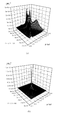
Figure 3:

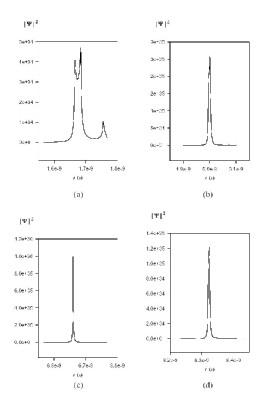
Figure 4:

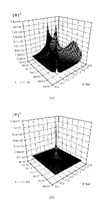
Figure 5:

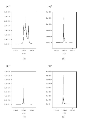
Figure 6:

Although the influence of the size of the aperture has been demonstrated only for the pulse given in Eq.(14), nevertheless one can easily extend the same analysis to spatio-temporally focused pulses of other types [cf. Eqs.(17),(20),(23)].

7. – Conclusions

In conclusion, by a generalization of the discrete “Temporal Focusing” method[23], we have found new classes of Superluminal waves. These new closed-form wave solutions show great potential for space-time focusing. Indeed, we can tailor initially spread-out pulses, so much so that they are strongly focused at a point chosen a priori in space-time. In this work we have demonstrated that these tailored pulses are easily adjustable by varying the velocity spectra of their Superluminal wave components.

We have also investigated the influence of having such pulses launched from a finite-size aperture. It has been shown that, because the individual Superluminal wave components, from which the focusing pulse is synthesized, have aperture-dependent diffraction-free lengths, the size of the aperture affects the focusing position and magnitude. The described method is very effective where all Superluminal wave components are propagating within their diffraction-free range.

Acknowledgements

The authors are very grateful to Hugo E.Hernández-Figueroa and K.Z.Nóbrega (FEEC, Unicamp), and to I.M.Besieris (Virginia Polytechnic Institute) for continuous discussions and collaboration. Useful discussions are moreover acknowledged with T.F.Arecchi, A.M.Attiya and C.A.Dartora, as well as with J.M.Madureira, S.Zamboni-Rached, V.Abate, F.Bassani, C.Becchi, M.Brambilla, C.Cocca, R.Collina, R.Colombi, C.Conti, G.C.Costa, G.Degli Antoni, L.C.Kretly, G.Kurizki, D.Mugnai, M.Pernici, V.Petrillo, A.Ranfagni, A.Salanti, G.Salesi, J.W.Swart, M.T.Vasconselos and M.Villa.

5. – Figure Captions

Fig.1 – Space-time evolution of the Superluminal pulse represented by Eq.(14); the parameter chosen values are $a=10^{-12}\;$s;  $V_{\rm min}=1.001\;c$;  $V_{\rm max}=1.005\;c$ while the focusing point is at $z_{\rm f}=200\;$cm.  One can see that this solution is associated with a rather good spatio-temporal focusing.  The field amplitude at $z=z_{\rm f}$ is 40.82 times larger than the initial one.  The field amplitude is normalized at the space-time point $\rho=0,\ z=z_{\rm f},\ t=t_{\rm f}$.

Fig.2 – Space-time evolution of the Superluminal pulse represented by Eq.(32). Now the parameters have the values $m=1$,  $a=10^{-12}\;$s (and therefore $\omega_{\rm c}=1\;$GHz);  $V_{\rm min}=1.001\;c$;  $V_{\rm max}=1.005\;c$); while the focussing point is again at $z_{\rm f}=200\;$cm.  Also this solution is associated with a very good spatio-temporal focusing:  The field amplitude at $z=z_{\rm f}$ is 1000 times higher than the initial one.  Once more, the field amplitude is normalized at the space-time point $\rho=0,\ z=z_{\rm f},\ t=t_{\rm f}$.

Figs.3. Surface plots of:  (a) the initial excitation $\big{|}\Psi\big{|}^{2}$ on the aperture plane $z^{\prime}=0$,  and  (b) the source-free pulse at the focusing point $z=z_{\rm f}=200$ cm. The spatio-temporally focused pulse corresponds to $a=10^{-12}$ s,  $V_{min\,}=1.001\;c$ and $V_{\rm max}=1.005\;c$. The radius of the aperture is chosen equal to 20 cm.

Figs.4 – The axial profiles of the field $\big{|}\Psi\big{|}^{2}$ radiated from a finite aperture at distances:  (a) $z=50$;  (b) 150;  (c) 200  and  (d) 250 cm. All other parameters are chosen as in Figs.4.

Figs.5 – Surface plots of:  (a) the initial excitation $\big{|}\Psi\big{|}^{2}$ on the aperture plane $z^{\prime}=0$,  and  (b) the source-free pulse at the  focusing point $z=z_{\rm f}=300$ cm. The spatio-temporally focused pulse has $a=10^{-12}$ s,  $V_{min\,}=1.001\;c$ and $V_{\rm max}=1.005\;c$. The radius of the aperture is chosen equal to 20 cm.

Figs.6 – The axial profiles of the field $\big{|}\Psi\big{|}^{2}$ radiated from a finite aperture at distances:  (a) $z=75$;  (b) 225;  (c) 285  and  (d) 375 cm. All other parameters are chosen as in Figs.6.

Bibliography:

[1] See, e.g., H.Bateman, Electrical and Optical Wave Motion (Cambridge Univ.Press; Cambridge, 1915);  J.A.Stratton, Electromagnetic Theory (McGraw-Hill; New York, 1941), p.356;  R.Courant and D.Hilbert, Methods of Mathematical Physics (J.Wiley; New York, 1966), vol.2, p.760.

[2] See, e.g., I.M.Besieris, A.M.Shaarawi and R.W.Ziolkowski, “A bi-directional traveling plane wave representation of exact solutions of the scalar wave equation”, J. Math. Phys., vol.30, pp.1254-1269, June 1989;  R.Donnelly and R.W.Ziolkowski, “Designing localized waves”, Proc. Roy. Soc. London A, vol.440, pp.541-565, March 1993.

[3] J.-y.Lu and J.F.Greenleaf, “Nondiffracting X-waves: Exact solutions to free-space scalar wave equation and their finite aperture realizations”, IEEE Trans. Ultrason. Ferroelectr. Freq. Control, vol.39, pp.19-31, Jan.1992.

[4] E.Recami, “On localized X-shaped Superluminal solutions to Maxwell equations”, Physica A, vol.252, pp.586-610, Apr.1998; and refs. therein.  For short review-articles, see, for instance, E.Recami, “Superluminal motions? A bird’s-eye view of the experimental situation”, Found. Phys., vol.31, pp.1119-1135, July 2001;  and Ref.[7].

[5] R.W.Ziolkowski, I.M.Besieris and A.M.Shaarawi, “Aperture realizations of exact solutions to homogeneous wave-equations”, J. Opt. Soc. Am., A, vol.10, pp.75-87, Jan.1993.

[6] M.Zamboni-Rached, E.Recami and H.E.Hernández F., “New localized Superluminal solutions to the wave equations with finite total energies and arbitrary frequencies”, Eur. Phys. J., D, vol.21, pp.217-228, Sept.2002.

[7] E.Recami, M.Z.Rached, K.Z.Nóbrega, C.A.Dartora & H.E.Hernández F.: “On the localized superluminal solutions to the Maxwell equations”, IEEE Journal of Selected Topics in Quantum Electronics, vol.9, issue no.1, pp.59-73, Jan.-Feb. 2003.

[8] See, e.g., J.-y.Lu, H.-h.Zou and J.F.Greenleaf, “Biomedical ultrasound beam forming”, Ultrasound in Medicine and Biology, vol.20, pp.403-428, 1994.

[9] P.Saari and H.Sõnajalg, “Pulsed Bessel beams”, Laser Phys., vol.7, pp.32-39, Jan.1997.

[10] M.Zamboni-Rached, K.Z.Nóbrega, H.E.Hernández-Figueroa and E.Recami, “Localized Superluminal solutions to the wave equation in (vacuum or) dispersive media, for arbitrary frequencies and with adjustable bandwidth” [e-print physics/0209101], in press in Opt. Commun.

[11] C.Conti, S.Trillo, P.Di Trapani, G.Valiulis, A.Piskarskas, O.Jedrkiewicz and J.Trull, “Nonlinear electromagnetic X-waves”, Phys. Rev. Lett., vol.90, paper no.170406, May 2003 [4 pages];  M.A.Porras, S.Trillo, C.Conti and P.Di Trapani, “Paraxial envelope X-waves”, Opt. Lett., vol.28, pp.1090-1092, July 2003.  

[12] A. M. Attiya, Transverse (TE) Electromagnetic X-waves: Propagation, Scattering, Diffraction and Generation Problems, Ph.D. Thesis, Cairo University, May 2001.

[13] See E.Recami, “Classical tachyons and possible applications”, Rivista N. Cim., vol.9(6), pp.1-178, 1986, issue no.6, and refs. therein;  A.O.Barut, G.D.Maccarrone and E.Recami, “On the shape of tachyons”, Nuovo Cimento A, vol.71, pp.509-533, Oct.1982.

[14] J.Fagerholm, A.T.Friberg, J.Huttunen, D.P.Morgan and M.M.Salomaa, “Angular-spectrum representation of nondiffracting X waves”, Phys. Rev., E, vol.54, pp.4347-4352, Oct.1996.

[15] J.-y.Lu and J.F.Greenleaf, “Experimental verification of nondiffracting X-waves”, IEEE Trans. Ultrason. Ferroelectr. Freq. Control, vol.39, pp.441-446, May 1992: In this case the beam speed is larger than the sound (not of the light) speed in the considered medium.

[16] P.Saari and K.Reivelt, “Evidence of X-shaped propagation-invariant localized light waves”, Phys. Rev. Lett., vol.79, pp.4135-4138, Nov.1997.

[17] D.Mugnai, A.Ranfagni and R.Ruggeri, “Observation of superluminal behaviors in wave propagation”, Phys. Rev. Lett., vol.84, pp.4830-4833, May 2000.

[18] P.Di Trapani, G.Valiulis, A.Piskarskas, O.Jedrkiewicz, J.Trull, C.Conti and S.Trillo, “Spontaneous formation of nonspreading X-shaped wavepackets”, e-print physics/0303083 (submitted for pub.).

[19] M.Z.Rached, E.Recami and F.Fontana, “Superluminal localized solutions to Maxwell equations propagating along a normal-sized waveguide”, Phys. Rev., E, vol.64, paper no.066603, Dec.2001 [six pages];  M.Z.Rached, F.Fontana and E.Recami, “Superluminal localized solutions to Maxwell equations propagating along a waveguide: The finite-energy case”, Phys. Rev., E, vol.67, paper no.036620, March 2003 [seven pages];  M.Z.Rached, K.Z.Nóbrega, E.Recami and H.E.Hernandez F., “Superluminal X-shaped beams propagating without distortion along a coaxial guide”, Phys. Rev., E, vol.66, 046617, Oct.2002 [ten pages];  M.Zamboni-Rached and H.E.Hernández-Figueroa, “A rigorous analysis of localized wave propagation in optical fibers”, Opt. Commun., vol.191, pp.49-54, May 2001.

[20] I.M.Besieris, M.Abdel-Rahman, A.Shaarawi and A.Chatzipetros, “Two fundamental representations of localized pulse solutions of the scalar wave equation”, Progress in Electromagnetic Research (PIER), vol.19, pp.1-48, 1998.

[21] S.He and J.y.Lu, “Sidelobe reduction of limited-diffraction beams with Chebyshev aperture apodization”, J. Acoust. Soc. Am., vol.107, pp.3556-3559, June 2000;  J.-y.Lu and S.He, “High frame rate imaging with a small number of array elements”, IEEE Trans. Ultrasound Ferroelec. Freq. Control, vol.46, pp.1416-1421, Nov.1999;  J.-y.Lu, “Experimental study of high frame rate imaging with limited-diffraction beams”, IEEE Trans. Ultrasound Ferroelec. Freq. Control, vol.45, pp.84-97, Jan.1998;  J.-y.Lu, “Producing bowtie limited-diffraction beams with synthetic array experiments”, IEEE Trans. Ultrasound Ferroelec. Freq. Control, vol.43, pp.893-900, Sep.1996;  J.-y.Lu and J.F.Greenleaf, “Producing deep depth of field and depth-independent resolution in NDE with limited-diffraction beams”, Ultrasonic Imaging, vol.15, pp.134-149, 1993.

[22] A.A. Chatzipetros, A.M. Shaarawi, I.M. Besieris and M. Abdel-Rahman, ”Aperture synthesis of time-limited X-waves and analysis of their propagation characteristics,” Journal of the Acoustical Society of America, vol. 103, pp.2287-2295, May 1998;  M. Abdel-Rahman, I.M. Besieris and A.M. Shaarawi, ”A comparative study on the reconstruction of localized pulses,” in Proceedings of the IEEE Southeast Conference (SOUTHEASTCON’97), pp.113-117 (Blacksburg, Virginia, April 1997).

[23] A.M.Shaarawi, I.M.Besieris and T.M.Said, “Temporal focusing by use of composite X-waves”, J. Opt. Soc. Am., A, vol.20, pp.1658-1665, Aug.2003.

[24] H.Sõnajalg, M.Rätsep and P.Saari, Opt. Lett., vol.22, p.310, 1997.

[25] I.S.Gradshteyn and I.M.Ryzhik, Integrals, Series and Products, 4th edition (Ac.Press; New York, 1965).

[26] A.T.Friberg, J.Fagerholm and M.M.Salomaa, “Space-frequency analysis of nondiffracting pulses”, Opt. Commun., vol.136, pp.207-212, March 1997;  J.Fagerholm, A.T.Friberg, J.Huttunen, D.P.Morgan and M.M.Salomaa, “Angular-spectrum representation of nondiffracting X waves”, Phys. Rev., E, vol.54, pp.4347-4352, Oct.1996;  P.Saari, in Time’s Arrows, Quantum Measurements and Superluminal Behavior, D.Mugnai et al. editors (C.N.R.; Rome, 2001), pp.37-48.

[27] D.Mugnai, A.Ranfagni and R.Ruggeri, “Pupils with super-resolution”, Phys. Lett., A, vol.31, pp.77-81, March 2003;  G.Toraldo di Francia, Supplem. Nuovo Cimento, vol.9, pag.426, 1952.