Classical Scattering for a driven inverted Gaussian potential in terms of the chaotic invariant set

Abstract

We study the classical electron scattering from a driven inverted Gaussian potential, an open system, in terms of its chaotic invariant set. This chaotic invariant set is described by a ternary horseshoe construction on an appropriate Poincare surface of section. We find the development parameters that describe the hyperbolic component of the chaotic invariant set. In addition, we show that the hierarchical structure of the fractal set of singularities of the scattering functions is the same as the structure of the chaotic invariant set. Finally, we construct a symbolic encoding of the hierarchical structure of the set of singularities of the scattering functions and use concepts from the thermodynamical formalism to obtain one of the measures of chaos of the fractal set of singularities, the topological entropy.

PACS numbers: 05.45.-a

I Introduction

Simple one-dimensional atomic potentials in external time-periodic electric fields have been used to predict several phenomena in the theory of laser-atom interactions at high laser intensity such as stabilization with increasing laser intensity. These models are of particular interest because their classical versions display chaotic motion Reichl , thus providing insight into quantum-classical correspondence.

The one-dimensional inverted Gaussian potential in the presence of a strong time-periodic electric field has already offered interesting insights into different aspects of the laser-atom interactions Bardsley ; Yao ; Marinescu . This short-range driven atomic potential has also been used to study the phase-space picture of resonance creation and to show that the resonance states are scarred on unstable periodic orbits of the classical motion Timberlake . In addition, two of the authors have studied electron scattering from the driven inverted Gaussian and, using Floquet theory, they constructed the Floquet scattering matrix. They found that the eigenphases of the Floquet scattering matrix undergo a number of ”avoiding crossings” as a function of the electron Floquet energy Agapi which is a quantum manifestation of the destruction of the constants of motion and the onset of chaos in classical phase space. These ”avoided crossings” were the motivating factor for a detailed study of the classical chaotic electron scattering from the driven inverted Gaussian potential which is the focus of the current work.

Of primary importance in chaotic scattering generalchaotic is the identification of universal features which distinguish it from regular scattering. For open systems, one such feature is the fractal set of singularities observed in scattering functions such as the time-delay function singularities . This fractal set of singularities is the result of the intersection of the incoming electron asymptotes with the invariant manifolds of the chaotic invariant set in the asymptotic region. The chaotic invariant set underlies the structure of the classical phase space in the sense that its properties determine the quantities which characterise the scattering process. One such property is the hierarchical structure of the chaotic invariant set which is the same as the structure of the fractal set of singularities of the time delay function.

In section IIIA of this paper, we obtain the hierarchical structure of the chaotic invariant set for the driven inverted Gaussian, which is an open system. The chaotic invariant set is represented as a horseshoe construction in an appropriate Poincare surface of section. We also obtain the development parameter of the horseshoe construction which describes the hyperbolic component of the invariant set while it ignores non-hyperbolic effects. In section IIIB we compute the time delay function and show that it has a fractal set of singularities with the same structure as the hierarchical structure of the invariant set. In section IIIC we obtain a symbolic dynamics symbolic1 ; symbolic6 , that is, a symbolic encoding of the branching tree, that describes the hierarchical structure of the chaotic invariant set and thus the hierarchical structure of the fractal set of singularities of the time delay function. Finally, using concepts from the thermodynamical formalism Beck ; Tel ; Feigenbaum , we obtain one of the measures of chaos of the fractal set of singularities of the scattering functions, the topological entropy.

II Model

We study the classical scattering of an electron from a one-dimensional inverted Gaussian atomic potential in the presence of a strong time-periodic electric field. The electric field $E(t)=E_{0}sin(\omega t)$ ($T=2\pi/\omega$ is the period of the field) is treated within the dipole approximation as a monochromatic infinite plane wave linearly polarized along the direction of the incident electron. In what follows, we work in the Kramers-Henneberger (KH) Kramers ; Henneberger frame of reference, which oscillates with a free electron in the time-periodic field. In the KH frame there are well defined asymptotic regions where the electron is under free motion. The Hamiltonian in one space dimension $x$ that describes the dynamics of the system in the KH frame is in atomic units (a.u.) Agapi

$$H(x,t)=\frac{p^{2}}{2}-V_{0}e^{-((x+\alpha(t))/\delta)^{2}},$$ (1)

where $\alpha(t)=\alpha_{0}sin(\omega t)$ is the classical displacement of a free electron from its center of oscillation in the time-periodic electric field $E(t)$ with $\alpha_{0}=-qE_{0}/\omega^{2}$ ($q$ is the particle charge which for the electron is $q=-1$ a.u.). Next, we transform Eq.(1) to a two-dimensional time-independent system, where the total energy $E$ of the system is conserved, as follows:

$$H=\frac{p^{2}}{2}-V_{0}e^{-((x+\alpha_{0}\sin(\phi))/\delta)^{2}}+\omega I.$$ (2)

$I$ and $\phi$ are respectively the action-angle variables of the driving field and $\phi=\omega t$. In the limit $x\rightarrow\pm\infty$ the Gaussian atomic potential tends to zero faster than $1/x$ Agapi . Thus, there are well defined asymptotic regions where the electron is under free motion and its dynamics is described by the asymptotic Hamiltonian:

$$H_{as}=\frac{p^{2}}{2}+\omega I.$$ (3)

In the asymptotic regime, Eq.(3), the electron momentum, $p$, as well as the action of the field, $I$, are conserved quantities. In the following sections, all our calculations are performed with the values $V_{0}=0.27035$ a.u. and $\delta=2$ a.u. assigned to the parameters of the inverted Gaussian potential. These values of the parameters $V_{0}$ and $\delta$ were shown to describe well the quantum behaviour of a one-dimensional model negative chlorine ion $Cl^{-}$ in the presence of a laser field Yao ; Marinescu ; Agapi ; Fearnside . The frequency of the time periodic field, $\omega$, and the amplitude of the field, $\alpha_{0}$, are taken constant and equal to $0.65$ a.u. and $0.9$ a.u., respectively. These values for the frequency and amplitude of the field were chosen so that the resulting horseshoe construction is not prohibitively complicated to study.

III Chaotic scattering

We are interested in understanding the underlying structure of the classical chaotic scattering system under consideration. That implies knowledge of the chaotic invariant set. In what follows, we first show how to construct the hierarchical structure of the chaotic invariant set for the inverted Gaussian atomic potential driven by a laser field. The scheme we follow to construct the hierarchical structure of the chaotic invariant set is valid only for systems with two degrees of freedom. Then, we show how the structure of the chaotic invariant set allows us to understand the structure of the fractal set of singularities of the scattering functions. We then obtain a symbolic dynamics for the hierarchical structure of the chaotic invariant set. This symbolic dynamics describes the hierarchical structure of the scattering functions as well. We express this symbolic dynamics in the form of a transfer matrix Feigenbaum and compute the topological entropy which in our case is a measure of the fractal structure of singularities of the scattering functions.

III.1 Chaotic invariant set

The chaotic invariant set is usually represented by a horseshoe construction in an appropriate Poincare surface of section. In the case of the well-known Smale horseshoe the construction is done by stretching a fundamental region $R$ and folding it on to the original region Smale ; Ott . The boundaries of $R$ are given by segments of the invariant manifolds of the outer fixed points of the system. Following the above general scheme we first define the fundamental region $R$. The system under consideration has three period-one periodic orbits (fixed points). The inner fixed point is an elliptic one. The two outer fixed points are located at $x\rightarrow\pm\infty$. As $x\rightarrow\infty$ the invariant stable and unstable manifolds of the outer fixed point $C$, see Fig.(1), converge to the same manifold (eigenvector), with $p=0$. The same is true for the manifolds of the fixed point $A$ at $x\rightarrow-\infty$. So, globally, the outer fixed points behave as unstable ones, that is, they produce invariant manifolds of the same topology as the one produced by hyperbolic fixed points. However, in a small neighbourhood around them they behave as parabolic ones. That is, the tangent map at $x\rightarrow\pm\infty$ has a degenerate eigenvalue equal to one (one eigenvector) Reichl . The invariant manifolds of these outer fixed points determine the boundaries of the fundamental area $R$, see Fig.(1).

In Fig.(1) the horseshoe is constructed on the Poincare surface of section $\phi=\pi/2$. We use the Poincare surface of section $\phi=\pi/2$ for all our calculations. This choice of the Poincare surface of section simplifies the horseshoe construction because on this plane the time reversal transformation $t\rightarrow-t$ is equivalent to the $p\rightarrow-p$ transformation. Thus, from the stable manifolds of the outer fixed points one obtains the unstable manifolds by letting $p\rightarrow-p$ and vice versa. The driven inverted Gaussian has no right/left symmetry. That is, the Hamiltonian is not invariant under the transformation $x\rightarrow-x$. Thus, the invariant set of the system is described by a ternary (three fixed points) asymmetric horseshoe construction. That is, the underlying structure of the scattering functions for electrons incident from the right/left is described by two different views right/left of the same horseshoe construction. The reason we consider the invariant manifolds of the outer fixed points is that these are the manifolds that are ”seen” by the scattering trajectories and thus have an effect on the scattering functions.

Let us now obtain the right view of the hierarchical structure of the horseshoe construction that underlies scattering for electrons incident from the right. The fundamental area $R$, see Fig.(1), is defined by the zero order tendrils as well as an infinite number of preimages/images of the unstable/stable invariant manifolds, respectively. We now add one iteration step of the stable manifolds. That is, using Hamilton’s equations of motion for the Hamiltonian given in Eq.(2) we propagate the points on the segments of the stable manifolds, $AD$ and $EC$ in Fig.(1), backwards in time for one period of the driving field (To obtain the tendrils of the unstable manifolds we propagate forward in time). The intersection of the first image, first order tendrils, of the stable manifolds with the unstable manifold of the fixed point $C$, segment $CD$ in Fig.(1), reveals the first order gap $G_{1}^{s}$, see Fig.(2). The intersection with the unstable manifold of one more iteration step of the stable manifolds reveals the second order gaps $G_{2}^{s}$, see Fig.(2). Thus, the gap $G_{n}^{s}$ is the area enclosed by the nth order tendril of the stable manifold and the boundary of the fundamental area $R$. A point that lies in $G_{n}^{s}$ is mapped out of the fundamental region after $n$ applications of the map, it is thus of hierarchy level $n$. These gaps play an important role because they are areas which are not needed to cover the invariant set. No higher level tendrils of the invariant manifolds will ever enter such gaps. So, with each iteration step one further tendril of the stable manifolds is added and one further level of hierarchy of these gaps is displayed Jung1 . We therefore see the construction scheme of the horseshoe by going from one level of hierarchy to the next. We note that the term gaps corresponds to what is known as lobes in fluid transport problems Wiggins . In particular, the gaps correspond to those lobes that are inside the area $R$. In a similar way, we construct the left view of the hierarchical structure of the horseshoe construction that underlies scattering for electrons incident from the left, see Fig.(2). The intersection points of the stable manifolds with the unstable manifolds of the outer fixed points, seen in Fig.(2) are the so called homoclinic/heteroclinic points for intersecting manifolds corresponding to the same (homoclinic) or different (heteroclinic) fixed points. These homoclinic/heteroclinic intersections underly the classical chaotic scattering.

Next, we compute the so called development parameter that approximately gives the development stage of the horseshoe construction. The significance of this parameter is that it describes universal aspects of the horseshoe and ignores the details. That is, it determines the hyperbolic component of the invariant set which is the important part for the scattering behaviour and neglects non-hyperbolic effects that are due to the Kolmogorov-Arnold-Moser (KAM) tori Jung1 ; Jung3 ; Jung4 . The non-hyperbolic effects appear at high levels of the hierarchy as tangencies, non transversal intersections, between stable and unstable manifolds and have a very small effect on the scattering functions (see symbolic6 for more details on tangencies between stable and unstable manifolds). For the values of the frequency and the amplitude of the driving field we choose, there are tangencies when $4$th, $n=4$, order tendrils of the stable manifolds are intersecting 4th order tendrils of the unstable manifolds in the interior of the fundamental region. The effect of these tangencies in the interior of the fundamental region becomes visible in the scattering functions at a hierarchical level $2n$, in our case 8. The reason is that if an $n$th order tendril of the stable manifold intersects tangentially an $n$th order tendril of the unstable manifold in the interior of the fundamental region, then the $n+1$ tendril of the stable manifold will intersect the $n-1$ tendril of the unstable manifold, and so on, until the $n+n$ tendril of the stable manifold intersects the zero order tendril of the unstable manifold, that is, when the $2n$ tendril of the stable manifold intersects the local segment (zero order tendril) of the unstable manifold. But, as we show in the next section, it is exactly the structure of the intersections of the stable manifolds with the local segment of the unstable manifold that is ”picked” by the scattering functions.

The development parameter has the value $1$ for a complete horseshoe. A horseshoe is complete when the tendril of level $1$ of the unstable manifold reaches the other side of the fundamental area $R$. For an incomplete horseshoe the development parameter is determined by the relative length of the tendril of level $1$ of the unstable manifold as compared to the complete case. It is given by $r_{n}N^{-n}$ Jung1 , where $n$ is the highest level of hierarchy considered, $r_{n}$ is the number of the gap that the tendril of order $1$ of the unstable manifold reaches up to, counting the gaps starting from the fixed point and N is the number of the fixed points. For the system under consideration $N=3$. It is important to realize that the numbers are assigned to the gaps of the incomplete horseshoe construction after comparing with the gaps of the complete horseshoe construction Jung1 . Note, that the value of the formal parameter, given by $r_{n}N^{-n}$, remains the same when different hierarchy levels are considered. The reason is, that as we go from a hierarchy level $n$ to the next hierarchy level $n+1$, $N-1$ gaps are added between successive gaps at the hierarchy level $n$, in the complete horseshoe construction. Thus, one can show that if the number $r_{n}$ is assigned to a certain gap at hierarchy level $n$, the number $r_{n+1}$ assigned to the same gap at hierarchy level $n+1$ is $r_{n+1}=Nr_{n}$. So, $r_{n+1}N^{-(n+1)}=r_{n}N^{-n}$ and the value of the formal parameter remains the same.

As already mentioned, for $\omega=0.65$ a.u. and $\alpha_{0}=0.9$ a.u. the driven inverted Gaussian is described by a ternary asymmetric horseshoe construction and it is thus described by two development parameters. The development parameter that corresponds to the manifolds of the fixed point at $x\rightarrow-\infty$, $A$, has the value $1$ since the first order tendril of the unstable manifold of the fixed point $A$ reaches the other side of the fundamental area $R$, see Fig.(2). The development parameter that corresponds to the manifolds of the fixed point at $x\rightarrow+\infty$, $C$, has the value $1/3$ as can be seen in Fig.(2). The value $1/3$ is obtained as follows: if we consider tendrils up to hierarchy level $n=1$ then the first order tendril of the unstable manifold of the fixed point $C$, $t_{1}^{u,C}$, reaches up to the $r=1$ gap. If we consider tendrils up to hierarchy level $n=2$ then $t_{1}^{u,C}$ reaches up to the $r=3$ gap and for hierarchy level $n=3$ $t_{1}^{u,C}$ reaches up to the $r=9$ gap. That is, the value of the development parameter remains the same when different hierarchy levels are considered. In Fig.(3), we see how the KAM tori around the middle fixed point cause an incomplete horseshoe construction. So for $\omega=0.65$ a.u. and $\alpha_{0}=0.9$ a.u. the chaotic invariant set is described by a ternary asymmetric horseshoe construction with development parameters $1$ and $1/3$. For reasons explained at the end of section II, the frequency is taken equal to 0.65 a.u. (high frequency regime compared to $V_{0}=0.27035$ a.u.). For this frequency a horseshoe with development parameters $1$ and $1/3$ is realized approximately in the interval $(0.7,1.15)$ a.u. of the amplitude of the field, $\alpha_{0}$.

III.2 Scattering functions

The scattering functions give properties of the final electron asymptotes as a function of the incoming electron asymptotes. In the case of classical chaotic scattering the scattering functions have a fractal set of singularities. This fractal set of singularities is the result of the intersection of the incoming electron asymptotes with the underlying chaotic invariant set. That is, when the scattering electron trajectory starts exactly on the stable manifold of the chaotic invariant set it stays on the chaotic set forever, resulting in a singularity of the scattering function. Furthermore, the structure of the set of singularities is the same as the structure of the chaotic invariant set Jung1 .

In what follows, we compute the time delay, $T^{del}$, one of the most important scattering functions. The time delay is a measure of how much the incoming electron delays due to its interaction with the potential in the scattering region and is given by:

$$T^{del}=T-|\frac{x_{in}}{p_{in}}|-|\frac{x_{out}}{p_{out}}|.$$ (4)

$T$ is the time it takes for the electron to travel from the incoming to the outgoing asymptotic region. There is an arbitrariness in the time $T$ due to the specific choice of the initial distance $x_{in}$ that the timing is initiated in the incoming asymptotic region and the final distance $x_{out}$ that the timing is stopped in the outgoing asymptotic region. To remove this arbitrariness we substract the time that the electron spends running along the initial and final asymptotes, $|\frac{x_{in}}{p_{in}}|$ and $|\frac{x_{out}}{p_{out}}|$ respectively.

We consider scattering from the right and compute the time delay function for a line of initial conditions in the asymptotic regime that completely intersects one tendril of the stable manifold of the outer fixed point $A$, see Fig.(4). We compute the time delay function, for the choice of initial conditions denoted as $0$ in Fig.(4), as a function of the initial momentum, $p_{in}$, along the line of initial conditions, see Fig.(5). This choice of initial conditions allows us to understand the structure of singularities of the time delay function as follows. From Fig.(4) we see that the iterates in time of the line of initial conditions converge toward the boundary of the fundamental region that is defined by the local segment of the unstable manifold of the fixed point $C$. The intersections of the line of initial conditions with the stable manifold of the fixed point $A$ are mapped on intersections of the iterates with the same stable manifold. Thus, the singularity structure of the scattering function is the same as the pattern resulting from the intersection of the stable manifolds with the local segment of the unstable manifold of the fixed point $C$. That implies that the intervals of continuity of the scattering function correspond to the gaps that the tendrils of the stable manifolds cut into the fundamental area of the horseshoe construction. In other words, the pattern of the fractal set of singularities of the time delay function is the same as the hierarchical structure of the horseshoe construction. We further illustrate this point as follows. In Fig.(6a), we compute the hierarchy level of the intervals of continuity for part of the time delay function, see Fig.(6b) (Fig.(6b) is a magnification of part of Fig.(5)). To do so, we initiate trajectories at the intervals of continuity of the delay function and count the number of times the scattering trajectories ”step” into the fundamental region, see Fig.(6a). If a scattering trajectory ”steps” inside the area $R$ $n-1$ times that means that it takes $n$ applications of the map before it is mapped outside of $R$. We thus say that the trajectory was initiated at an interval of continuity of hierarchy level $n$. For example, we see from Fig.(6a) that the scattering trajectory with $p_{in}=-0.1973$ ”steps” two times inside $R$. Thus, the interval of continuity it was initiated at is of hierarchy level three. The resulting pattern of singularities shown in Fig.(6a) is the same as the pattern of singularities of the time delay function as a comparison of Figs.(6a) and (6b) reveals.

Let us now explain how the hierarchy level of the intervals of continuity is related to the gaps of the horseshoe construction. As we illustrate in Fig.(7), if a scattering trajectory approaches the local segment of the unstable manifold along a gap of order $n$, then it steps inside the area $R$ $n-1$ times before it is mapped outside $R$. At the same time, if the scattering trajectory steps inside the area $R$ $n-1$ times that means that it is mapped outside of $R$ after $n$ applications of the map and thus the trajectory was initiated at an interval of continuity of hierarchy level $n$. Thus, a gap of hierarchy level $n$ of the horseshoe construction corresponds to an interval of continuity of hierarchy level $n$ of the time delay function. That implies that the hierarchical structure of the chaotic invariant set and of the scattering functions is the same. Indeed, a comparison of Figs.(6a) and (9) (Fig.(9) is explained in the following section) reveals that the pattern of singularities of the time delay function in Fig.(6b) is the same as that part of the hierarchical structure of the chaotic invariant set that is encircled by a square in Fig.(9).

For the system under consideration the potential in the interaction region is known and so we can directly obtain the hierarchical structure of the chaotic invariant set and thus the structure of the scattering functions. However, when the potential in the interaction region is not known, then one has to find from asymptotic observations the hierarchical structure of the scattering functions in order to obtain the structure of the chaotic invariant set.

III.3 Measures of Chaos

It is possible to construct a topological measure of the degree of chaos contained in this scattering system if we can construct a symbolic dynamics which reproduces the hierarchy of intersections of the stable and unstable manifolds. The first step is to obtain the branching trees that describe the right/left view of the horseshoe constructions for scattering from the right/left respectively. The second step involves the development of a symbolic dynamics which reproduces the structure of the branching trees. It is important to note that for the values of the amplitude and the frequency of the driving field considered there are tangencies between the stable and unstable manifolds on the 4th order tendrils. These tangencies introduce non-hyperbolic effects that will cause a breakdown of the symbolic dynamics starting from hierarchy level $8$ and higher. However, knowledge of the symbolic dynamics up to hierarchy level 8 gives a significant measure of the degree of observable chaos in this scattering system.

III.3.1 Branching Trees

Let us first obtain a branching tree Jung1 , that describes the right view of the horseshoe construction for scattering from the right. We will use information developed in Section IIIA. First, let us consider the interval $I_{1}^{0}$ which corresponds to the local segment of the unstable manifold $CD$ of the fixed point $C$ (see Fig.(8)). This is the first step in the construction of the branching tree and corresponds to hierarchy level $n=0$. In the second step, hierarchy level n=1, the first order tendril of the stable manifold of the fixed point $A$ cuts the interval $(s_{0},s_{1})$ out of $I_{1}^{0}$ and leaves two intervals $I_{1}^{1}$ (the segment of $CD$ from $D$ to $s_{0}$) and $I_{2}^{1}$ (the segment of $CD$ from $s_{1}$ to $C$). In the third step, hierarchy level $n=2$, the second order tendril of the stable manifold of the fixed point $A$ cuts the interval $(s_{4},s_{5})$ out of $I_{2}^{1}$ and leaves two intervals, $I_{21}^{2}$ (the segment of $CD$ from $s_{1}$ to $s_{4}$) and $I_{22}^{2}$ (the segment of $CD$ from $s_{5}$ to $C$). In the same step (the same iteration) the second order tendril of the stable manifold of the fixed point $C$ cuts the interval $(s_{2},s_{3})$ out of $I_{1}^{1}$ and leaves two intervals, $I_{11}^{2}$ (the segment of $CD$ from $D$ to $s_{2}$) and $I_{12}^{2}$ (the segment of $CD$ from $s_{3}$ to $s_{0}$). Continuing this process we obtain the branching tree shown in Fig.(9).

In a similar way, we construct the branching tree that describes the left view of the horseshoe construction for scattering from the left, see Fig.(10). The hierarchical structure of these branching trees is the same as the hierarchical structure of the chaotic invariant set.

III.3.2 Symbolic Dynamics

Having determined the geometry of the branching trees, we can now construct a symbolic dynamics that encodes the branching trees. In principle, since we have a non-hyperbolic horseshoe construction one needs an infinite number of grammatical rules to construct a symbolic dynamics. However, we can construct an approximate symbolic dynamics that describes well the outermost hyperbolic component of the horseshoe construction. The symbolic encoding of the branching tree is not unique, but the measures of chaos one obtains for different encodings are the same.

Our symbolic dynamics consists of four symbol values A,B,C and + and a set of grammatical rules that allow us to encode each branch of the branching tree. That is, each branch of the tree of hierarchy level n, is labeled by a vertical sequence (string) of $n$ symbols made out of the four symbol values A,B,C, and +. Each symbol sequence is read vertically up the branch of the tree (see Figs.(9) and (10)). The order in which the four symbol values appear in each branch of the tree is determined by the grammatical rules. That is, the rules tell us which of the four symbol values are allowed to be appended to a given branch of the tree as we go from a certain hierarchy level to the next.

Our rules depend on the last ”word” that appears on a given branch. This ”word” is a vertical sequence of one two or three symbols and can be either of the eleven ”words”: A, ++, B+C, C+C, ++C, CC, BC, AC, B, B+ and C+ (see Figs.(9) and (10)). The rules are:

• After a string (branch) ending in $A$, $B+C$, $C+C$ or $++$ it is allowed to attach the symbols $A$, $B$ and $C$, going from left to right (standard orientation). Thus, three strings (branches) stem out ending in $A$, $B$ and $C$.

• After a string (branch) ending in $AC$, $B$, $BC$, $B+$, $C+$, $CC$ or $++C$ it is allowed to attach the symbols $+$ and $C$, going from left to right (standard orientation). Thus, two strings (branches) stem out ending in $+$, $C$.

• $B$ always inverts the previous orientation.

• $C$ always inverts the previous orientation if it comes after $S+$, where $S$ is not $+$.

• $+$ always inverts the previous orientation if it comes after $S$ where $S$ is not $+$.

By previous orientation we mean the following: if at a hierarchy level $n$ there are three branches ending, for example, in the symbols $A$, $B$ and $C$, going from left to right (see Fig.(10)), then at hierarchy level $n+1$, from the string ending in $B$ two strings stem out with symbol endings $+$ and $C$, according to the second grammatical rule. According to the third grammatical rule, the symbol endings $+$ and $C$, going from left to right, at level $n+1$, must have the inverse orientation to the one of the symbol endings at level $n$. In this example, at level $n$, the symbol endings $A$, $B$ and $C$, going from left to right, have the standard orientation. Thus, after the string ending in $B$, two branches stem out, at level $n+1$, with symbol endings $C$ and $+$, going from left to right, see Fig.(10).

To symbolically encode the right/left branching trees in Figs.(9) and (10) we have started at level $n=1$ by attaching the symbols $+$ and $C$ for the right and $A$, $B$ and $C$ for the left view of the branching trees, respectively, and then use the above grammatical rules to continue the encoding. Using these rules we can encode and thus obtain the structure of the branching trees safely up to hierarchy level 7. For the values of the frequency and amplitude of the driving field we consider here, there are tangencies between the invariant manifolds at level four in the interior of the fundamental region. These tangencies can cause our symbolic encoding to break down at hierarchy level 8 and higher of the branching tree. That is, these tangencies can introduce additional branches in the branching tree, starting at level 8, which are not accounted for by our grammatical rules. Note, that the above described symbolic dynamics encodes the branching trees of the scattering functions as well.

If we now use concepts from a thermodynamical formalism Beck ; Tel , we can express the above described grammatical rules in the form of a transfer matrix Feigenbaum . To construct the transfer matrix we use as entries the eleven ”words” listed earlier. The matrix element $(l,m)$ is $1$ if it is possible to attach to the ”word” $l$ a symbol such that the resulting string ending is the ”word” $m$, otherwise the matrix element is $0$. In other words, if the transfer matrix element $(l,m)$ is one it means that if at a certain hierarchy level we have a string ending in the ”word” $l$ when we go to the next hierarchy level it is allowed to encounter a string ending in the ”word” $m$. To clarify this point, consider for example the string ending with the ”word” $l=++$ (see Fig.(11)). According to the first grammatical rule, after the ”word” $++$ we can attach three symbols labeled $A$, $B$ and $C$ and so obtain the strings $++A$, $++B$ and $++C$. These strings have the string endings, $m=A$, $m=B$ and $m=++C$, respectively, which can be identified with three of the eleven ”words”. Thus, the matrix elements $(++,A)$, $(++,B)$ and $(++,++C)$ are one, while all other matrix elements with $l=++$ are $0$.

Having constructed the transfer matrix, we can now compute the topological entropy of the branching tree. The topological entropy is a measure of the degree of chaos in the scattering system. Let us first describe the relation between the topological entropy and the transfer matrix. The topological entropy $K_{0}$ is the rate of exponential growth of the number of intervals $Z(n)$, or equivalently the number of branches $Z(n)$, at a hierarchical level $n$ when $n$ is large with $Z(n)=e^{nK_{0}}$ Beck . It directly follows that $K_{0}=ln(Z(n+1)/Z(n))$. But, for large $n$, $Z(n+1)/Z(n)$ is the average branching ratio of the trees. This ratio is given by the largest eigenvalue of the transfer matrix Feigenbaum . For our system, the largest eigenvalue is $\approx 2.31$. Thus, the topological entropy of the branching tree is $K_{0}\approx 0.84$. This topological entropy describes the rate of growth of the branches in the hierarchical structure of the scattering functions and is thus a measure of chaos of the fractal set of singularities.

It is useful to mention that for a horseshoe with $N$ fixed points the value of the topological entropy, $K_{0}$, can vary between $0$ and $ln(N)$. This is easily understood, since for a horseshoe with $N$ fixed points the maximum value of the average branching ratio is $N$ and $K_{0}$ is the logarithm of the average branching ratio. Thus, for a ternary horseshoe construction, the case currently under consideration, $K_{0}$ can vary between $0$ and $ln(3)\approx 1.1$. For the values of the frequency and amplitude of the driving field considered in this paper, we find that $K_{0}\approx 0.84$, close to the maximum value of $1.1$, which suggests that our system is in the regime of strong chaos.

IV Conclusions

In this paper, we have studied the classical electron scattering from a driven inverted Gaussian potential which is an open system. We have shown that the fractal pattern of singularities of the scattering functions can be understood in terms of the hierarchical structure of the chaotic invariant set which underlies the chaotic dynamics. We have constructed a symbolic encoding of the hierarchical structure of the chaotic invariant set. Using concepts from the thermodynamical formalism, we have used this encoding to obtain the topological entropy of the fractal set of singularities of the scattering functions.

List of Figures

• Fig1. The fundamental region $R$ is formed by the unstable manifold of the fixed point $A$, segment $AE$, by the stable manifold of the fixed point $C$, segment $CE$, by the unstable manifold of the fixed point $C$, segment $CD$, and the stable manifold of the fixed point $A$, segment $AD$.

• Fig2. Horseshoe construction up to hierarchy level two on the Poincare surface of section $\phi=\pi/2$. The solid lines indicate tendrils of order zero, the dashed lines indicate tendrils of order one and the dotted lines indicate tendrils of order two. The gaps $G_{n}^{s}$ on the bottom right/top left are formed by intersections of the stable manifolds of the fixed points $A$ and $C$ with the local segment of the unstable manifold of the fixed point $C$/$A$, that is, $CD$/ $AE$. These intersections describe the right view/left view of the horseshoe construction. $t_{1}^{u,A}$ indicates the first order tendril of the unstable manifold of the fixed point $A$. $t_{1}^{u,C}$ indicates the first order tendril of the unstable manifold of the fixed point $C$.

• Fig3. The initial conditions used to generate this strobe plot lie on the line $p=0$. This strobe plot is generated by evolving the trajectories forward in time and it thus ”picks” the unstable manifolds of the fixed points $A$ and $C$. The location of the middle fixed point, $B$, (period-1 orbit) is located at $x=0.29$ and is indicated by a filled rectangle. Comparing with Fig.(1), we see that the first order tendril of the unstable manifold of the fixed point $A$, $t_{1}^{u,A}$, penetrates the fundamental area $R$ completely. In the case though of the first order tendril of the unstable manifold of the fixed point $C$, $t_{1}^{u,C}$, the KAM tori around the fixed point $B$ prevents it from reaching the boundary of the fundamental area $R$.

• Fig4. For scattering from the right, we indicate as $0$ the line of initial conditions in the asymptotic region used to compute the time delay function. This set of initial conditions intersects the stable manifold of the fixed point $A$. The numbers $1-4$ indicate successive iterations in time of the set of initial conditions.

• Fig5. Time delay function as a function of the initial momentum for the set of initial conditions shown in Fig.(4).

• Fig6. In a) we show the hierarchy level of the intervals of continuity for part of the time delay function, see Fig.(5). For a given pair of initial values, $x_{0},p_{0}$, we propagate the trajectories until they reach one of the asymptotic regions and count the number of times the trajectory steps in the fundamental area $R$. In b) we plot the time delay function for the same range of initial conditions as for the hierarchy level of the intervals of continuity shown in a). We can immediately see that both functions have the same pattern of singularities.

• Fig7. The solid lines indicate tendrils of order zero, the dashed lines tendrils of order one, the dotted lines tendrils of order two and the dashed-dot line tendrils of order three. We initiate a trajectory in the right asymptotic region with $p_{in}=-0.1973$ which is inside an interval of continuity, see Fig.(6a). We then successively iterate the trajectory in time (stars). The successive iterations are indicated by numbers 1-8, respectively. The trajectory approaches the local segment $CD$ of the unstable manifold of the fixed point $C$ inside the third order tendril of the stable manifold of the fixed point $A$ along a third order gap. One more iteration in time maps area $a$ (shaded by dots), which is enclosed by the third order tendril of the stable manifold of the fixed point $A$ and its unstable manifold, into area $b$ (shaded by lines), which is enclosed by the second order tendril of the stable manifold of point $A$ and its unstable manifold. A further iteration in time maps area $b$ into area $c$ (shaded by lines), which is enclosed by the first order tendril of the stable manifold of point $A$ and its unstable manifold. Finally, area $c$ is mapped to area $d$ (shaded by lines) and enclosed by the zero order tendril of the stable manifold of point $A$ and its unstable manifold. But area $d$ is outside the fundamental region and thus the trajectory steps inside the fundamental region two times. Generally, if the scattering trajectory approaches the local segment of the unstable manifold along a gap of hierarchical order n it will ”step” inside the fundamental area, $R$, n-1 times before it is mapped outside $R$.

• Fig8. Construction of the branching tree for scattering from the right. The first order gap $G_{1}^{s}$ reduces the initial interval $I_{1}^{0}$, at hierarchy level $n=0$, down to the two intervals $I_{1}^{1}$ and $I_{2}^{1}$. Note that for the scattering functions, we obtain exactly the same branching tree as for the chaotic invariant set. For the scattering functions, instead of the gaps it is the intervals of continuity that are cut out from the original interval in a Cantor set structure.

• Fig9. Branching tree and symbolic dynamics for scattering from the right shown up to hierarchy level four. Each interval corresponds to one branch of the tree. A branch at hierarchy level $n$ is described by a string of length $n$.

• Fig10. Branching tree and symbolic dynamics for scattering from the left shown up to hierarchy level four. Let us now explain what we mean by previous orientation in terms for example of the third grammatical rule. For example, at the hierarchical level $n=2$, indicated by the arrow, the symbol endings of the three branches going from left to right are $A$, $B$ and $C$ which is what we define as standard orientation. After the symbol value $B$ we can attach the symbols $+$ and $C$ at the hierarchical level $n=3$, indicated again by an arrow. According to the third grammatical rule the symbols $+$ and $C$, at level $n=3$, will be attached, after $B$, so that they have the inverse orientation of the symbol values at level $n=2$. So, since at level $n=2$ the symbols $A$, $B$ and $C$ are attached in standard orientation then at level $n=3$ we attach after $B$ symbols $C$ and $+$ going form left to right, resulting in an inverse orientation compared to the one at level $n=2$. Thus, we say that $B$ always inverts the previous orientation.

• Fig11. Transfer matrix.

Figure 1:

Figure 2:

Figure 3:

Figure 4:

Figure 5:

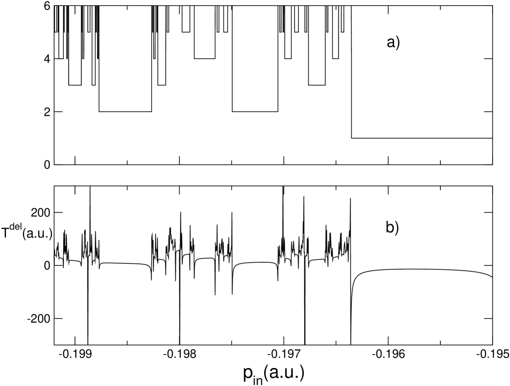
Figure 6:

Figure 7:

Figure 8:

Figure 9:

Figure 10:

Figure 11:

References

- (1) L. E. Reichl, The Transition to Chaos In Conservative Classical Systems: Quantum Manifestations (Springer-Verlag, Berlin, 1983).
- (2) J. N. Bardsley and M. J. Comells, Phys. Rev. A 39, 2252 (1989).
- (3) G. Yao and S.-I. Chu, Phys. Rev A 45, 6735 (1992).
- (4) M. Marinescu and M. Gavrila, Phys. Rev. A 53, 2513 (1996).
- (5) T. Timberlake and L. E. Reichl, Phys. Rev. A 64, 033404 (2001).
- (6) A. Emmanouilidou and L. E. Reichl, Phys. Rev. A 65, 033405 (2002).
- (7) B. Eckhardt, Physica D 33, 89 (1988); U. Smilansky, 1992, Proc. 1989 Les Houches Summer School ed. M. J. Giannoni, A. Voros and J. Zinn-Justin (Amsterdam: North-Holland) pp 371-441; E. Ott and T.Tl, Chaos 3, 417 (1993); Z. Kovcs and L. Wiesenfeld, Phys. Rev. E 51, 5476 (1995).
- (8) C. Jung and H. J. Scholz, J. Phys. A: Math. Gen. 20, 3607 (1987); T. Tl Phys. Rev. A 36, 1502 (1987).
- (9) P. Cvitanovic, G. Gunaratne and I. Procaccia, Phys. Rev. A 38, 1503 (1988); D. Auerbach and I. Procaccia, Phys. Rev. A 41, 6602; C. Jung and P. Richter, J. Phys. A: Math. Gen. 23, 2847; G. Troll, Physica D 50, 276, (1991); J. Vollmer and W. Breymann, Helv. Phys. Acta 66, 91 (1993).
- (10) B. Rckerl and C. Jung, J. Phys. A: Math. Gen. 27, 55 (1994).
- (11) C. Beck and F. Schlogel, Thermodynamics of chaotic systems, Cambridge Univ. Press, Cambridge, UK, 1993 (sections 8.4 and 17.5).
- (12) G. Karolyi and T. Tl, Physics Reports 290, 125 (1997).
- (13) M. J. Feigenbaum, M. H. Jensen and I. Procaccia, Phys. Rev. Lett. 57, 1503 (1986).
- (14) H. A. Kramers, Collected Scientific Papers (North-Holland, Amsterdam, 1956), p.272.
- (15) W. C. Henneberger, Phys. Rev. Lett. 21, 838 (1968).
- (16) A. S. Fearnide, R. M. Portvliege, and R. Shakeshaft, Phys. Rev. A 51, 1471 (1995).
- (17) S. Smale, Bull. Am. Math. Soc. 73, 747 (1967).
- (18) E. Ott, Chaos in Dynamical Systems, Cambridge Univ. Press, Cambridge, UK, 1993.
- (19) C. Jung, C. Lipp and T. H. Seligman, Annals of Physics 275, 151 (1999).
- (20) D. Bigie, A. Leonard and S. Wiggins, Nonlinearity 4, 775 (1991).
- (21) B. Rckerl and C. Jung, J. Phys. A 27, 6741 (1994).
- (22) W. Breymann and C. Jung, Europhys. Lett. 25, 509 (1994).