Localized wave solutions of the scalar homogeneous wave equation and their optical implementation

Abstract

In recent years the topic of localized wave solutions of the homogeneous scalar wave equation, i.e., the wave fields that propagate without any appreciable spread or drop in intensity, has been discussed in many aspects in numerous publications. In this review the main results of this rather disperse theoretical material are presented in a single mathematical representation - the Fourier decomposition by means of angular spectrum of plane waves. This unified description is shown to lead to a transparent physical understanding of the phenomenon as such and yield the means of optical generation of such wave fields.

year number number identifier LABEL:FirstPage1 LABEL:LastPage#12

I INTRODUCTION

The birth of the diffraction theory of light dates back to the works of Francis Maria Grimaldi (1618 – 1663), Robert Hook (1635 – 1703), Christiaan Huygens (1629 – 1695) and Thomas Young (1773 – 1829) and was mathematically formulated by Augustin Jean Fresnel (1788 – 1827). Over the two centuries it has been considered as a very successful theory – it indeed very precisely describes the propagation of light in linear media. The foundation of the diffraction theory is the principle of Huygens which states that (i) all the points of a wavefront act as the sources of secondary wavelets and (ii) the field at all the subsequent points is determined by the superposition of those wavelets.

The topic of free-space propagation of wave fields has attracted a renewed interest in 1983 when James Neill Brittingham claimed fw1 that he discovered a family of three-dimensional, nondispersive, source-free, free-space, classical electromagnetic pulses which propagate in a straight line in free space at light velocity (in this work he also introduced the term focus wave mode (FWM) for those wave fields). Now, the very idea of secondary spherical sources in the classical diffraction theory implies that any optical wave field suffers from lateral and longitudinal spread in the course of propagation in free space, whereby the diffraction angle of the spread is the larger the narrower is the field radius. In the view of this general principle the Brittingham’s statement is an astounding one and he quite rightly used the formula ”to convince the scientific community” in its arguments. However, the original focus wave mode was indeed the solutions of the Maxwell’s equations and the scientific community had to resolve this apparent contradiction. As to give the reader an idea of the initial problem the theoreticians had to tackle with, we reproduce here the original definition of Brittingham which he deduced by ”a very extensive heuristical fit of various differential equation solutions”: given the Maxwell equations (SI)

$$\mathbf{\nabla\times E} =-\dfrac{\partial\mathbf{B}}{\partial t}$$

$$\mathbf{\nabla\times H} =\dfrac{\partial\mathbf{D}}{\partial t}$$

$$\mathbf{\nabla\cdot D} =0$$

$$\mathbf{\nabla\cdot B} =0\text{,}$$

 where $\mathbf{E}$, $\mathbf{D}$, $\mathbf{H}$, $\mathbf{B}$ and $t$ are electric field, electric flux density, magnetic field, magnetic induction and time variable, respectively and using cylindrical coordinate system ($\rho,\varphi,z-ct$) the mathematical formulation of the original FWM reads as

$$D_{\rho}\left(\rho,\varphi,z,t\right) =\Psi_{1}+\Psi_{1}^{\ast}$$

$$D_{\varphi}\left(\rho,\varphi,z,t\right) =\Psi_{2}+\Psi_{2}^{\ast}$$

$$H_{\rho}\left(\rho,\varphi,z,t\right) =\Psi_{3}+\Psi_{3}^{\ast}$$

$$H_{\varphi}\left(\rho,\varphi,z,t\right) =\Psi_{4}+\Psi_{4}^{\ast}$$

$$H_{z}\left(\rho,\varphi,z,t\right) =\Psi_{5}+\Psi_{5}^{\ast}\text{,}$$

where the functions $\Psi_{q}$ ($q=1,2...5$) are written as

$$\Psi_{q}=A_{q}\left(\rho,z-ct\right)G_{1}\left(\rho,z-ct\right)G_{2}\left(z-ct\right)G_{3}\left(z-c_{1}t\right)\Phi^{\prime}\left(\phi\right)$$

for $q=1$ and $4$, and

$$\Psi_{q}=A_{q}\left(\rho,z-ct\right)G_{1}\left(\rho,z-ct\right)G_{2}\left(z-ct\right)G_{3}\left(z-c_{1}t\right)\Phi\left(\phi\right)$$

for $q=2,3,5$. In those equations

$$G_{1} =\exp\left[-\frac{\rho^{2}}{4F}\right]$$

$$G_{2} =\exp\left[-ik_{1}\left(z-ct\right)\right]$$

$$G_{3} =\exp\left[ik_{2}\left(z-c_{1}t\right)\right]$$

and

$$F=ig\left(z-ct\right)+\xi\text{~{}.}$$

The remaining definitions read as

$$A_{1}=\frac{D^{TE}}{c^{2}}\left[\frac{\left(n+1\right)cg\rho^{n-1}}{F^{n+2}}-\frac{cg\rho^{n+1}}{4F^{n+3}}+\frac{\left(k_{1}c-k_{2}c\right)\rho^{n-1}}{F^{n+2}}\right]$$

$$A_{2} =-\frac{D^{TE}}{c^{2}}\left[\frac{n\left(n+1\right)cg\rho^{n-1}}{F^{n+2}}-\frac{\left(3n+4\right)cg\rho^{n+1}}{4F^{n+3}}\right.$$

$$+\frac{n\left(k_{1}c-k_{2}c_{1}\right)\rho^{n-1}}{F^{n+1}}$$

$$\left.+\frac{2cg\rho^{n+3}}{16F^{n+4}}-\frac{2\left(k_{1}c-k_{2}c_{1}\right)\rho^{n+1}}{4F^{n+2}}\right]$$

$$A_{3} =-\frac{D^{TE}}{c^{2}}\left[-\frac{n\left(n+1\right)g\rho^{n-1}}{F^{n+2}}+\frac{\left(3n+4\right)g\rho^{n+1}}{4F^{n+3}}\right.$$

$$+\frac{n\left(-k_{1}+k_{2}\right)\rho^{n-1}}{F^{n+1}}$$

$$\left.-\frac{2g\rho^{n+3}}{16F^{n+4}}-\frac{2\left(-k_{1}+k_{2}\right)\rho^{n+1}}{4F^{n+2}}\right]$$

$$A_{4} =-D^{TE}\left[-\frac{\left(n+1\right)g\rho^{n-1}}{F^{n+2}}+\frac{g\rho^{n+1}}{4F^{n+3}}\right.$$

$$\left.+\frac{\left(-k_{1}+k_{2}\right)\rho^{n-1}}{F^{n+1}}\right]$$

$$A_{5}=-iD^{TE}\left[\frac{\rho^{n+2}}{4F^{n+3}}-\frac{\left(n+1\right)\rho^{n}}{F^{n+2}}\right]~{}\text{,}$$

where $D^{TE}$, $g$, $\xi$, $k_{1}$ and $k_{2}$ are constants. The $\Phi$ functions are defined as

$$\Phi\left(\varphi\right) =\left\{\begin{array}[c]{c}\sin\left(n\varphi\right)\\ \cos\left(n\varphi\right)\end{array}\right\}$$

$$\Phi^{\prime}\left(\varphi\right) =\left\{\begin{array}[c]{c}n\cos\left(n\varphi\right)\\ -n\sin\left(n\varphi\right)\end{array}\right\}$$

and the supplemental conditions read

$$2gk_{2}d_{1} =1$$

$$k_{2}^{2}d_{2} =\frac{k_{1}}{g}\text{,}$$

where

$$d_{1} =\left(1-\frac{c_{1}}{c}\right)$$

$$d_{2} =\left(1-\frac{c_{1}^{2}}{c^{2}}\right)\text{.}$$

One has to agree, that the physical idea is very much hidden behind this mathematical formulation.

Brittingham claimed, that this mathematical formulation (i) satisfy the homogeneous Maxwell’s equations, (ii) is continuous and nonsingular, (iii) has a three-dimensional pulse structure, (iv) is nondispersive for all time, (v) move at light velocity in straight lines, and (vi) carry finite electromagnetic energy. Thus, the formulas above give a mathematical formulation of a free-space wave field that can be described as a ”light bullet” and, though the proof of the last claim was shown to be faulty by Wu and King fw2 , the whole idea was very intricate and rose a considerable scientific interest fw3 –ok6 .

The theoretical work of following years could be divided into the following topics (see also Ref. lw6 for an overview):

In the following publications fw3 ; fw5 the original vector field was reduced to its scalar counterpart and the dominant part of the research work that followed has been formulated in terms of solutions to homogeneous scalar wave equation.

The close connection between the FWM’s and the solutions of the paraxial wave equation and Schrödinger’s equation (which both allow localized solutions) has been established fw3 ; fw4 ; fw5 – it has been shown that in terms of the variables $z+ct$ and $z-ct$, if the solution of the scalar wave equation is given by the anzatz $\exp\left[\beta\left(z+ct\right)\right]F\left(x,y,z-ct\right)$, the problem can be reduced to one of those equations.

The infinite energy content of the original FWM’s has been addressed in several publications (see Refs. fw3 ; fw3o1 ; fw5 ; fw14 ; fw16 ; lw1 ; g1 ; g2 ; g3 ; g4 ; g5 and references therein). First of all, Sezginer fw3 and Wu and Lehmann fw3o1 proved that any finite energy solution of the wave equation irreversibly leads to dispersion and to spread of the energy. Then Ziolkowski fw5 pointed out, that the superpositions of the infinite energy FWM’s could result in finite energy solutions and in following publications a number of finite energy solutions to the scalar wave equation and Maxwell equations were deduced – ”electromagnetic directed-energy pulse trains” (EDEPT) lw1 ; g1 , ”acoustic directed-energy pulse trains” (ADEPT) g0b , splash pulses fw5 , modified power spectrum (MPS) lw1 pulses, electromagnetic missiles mis1 ; mis2 , various super- and subluminal pulses fw15 etc. In correspondence with fw3 ; fw3o1 this broader class of localized waves (LW) have generally extended but finite ranges of localizations. Also, several alternate infinite energy LW’s (Bessel-Gauss pulses lw4 for example) were deduced.

In Ref. fw14 Besieris et al introduced a novel integral representation for synthesizing those LW’s. This bidirectional plane wave decomposition is based on a decomposition of the solutions of the scalar wave equations into the forward and backward traveling plane wave solutions and it has been shown to be a very natural basis for description of LW’s (see Ref. lw1 for example).

The FWM’s have been interpreted as being related in a special way to the field of a source, moving on a complex trajectory parallel to the real axis of propagation fw5 ; fw11 ; fw13 ; lw1 . This observation linked the FWM’s with the works by Deschamps o4 and Felsen o5 where the Gaussian beams have been described as being paraxially equivalent to spherical waves with centers at stationary complex locations.

There has been a considerable effort in finding the LW solutions in other branches of physics, spanning various differential equations like spinor wave equation fwz5 , fist-order hyperbolic systems like cold-plasma equation fwz10 , Klein-Gordon equation fw14 ; fw15 .

In 1988 Durnin b1 published his paper on so called Bessel beams (see for example Ref. bag5 for an earlier publication on the topic). The idea attracted much interest and the Bessel beams and their pulsed counterparts – X-waves x1 –x20 and Bessel-X waves bx1 ; bx2 ; bx5  – became the research field of its own rights. In this context the issue of the superluminal propagation of a class of LW’s has been considered in Refs. x7 ; x50 ; x55k ; x56k ; x57k ; x60k ; x70k .

It has been shown that the FWM’s can be described as monochromatic Gaussian beams observed in a moving relativistic inertial reference frame fw6 ; lw6 .

Propagation of optical pulses or beams without any appreciable drop in the intensity and spread over long distances would be highly desirable in many applications. The obvious uses could be in fields like optical communication, monitoring, imaging, and femtosecond laser spectroscopy, also in laser acceleration of charged particles. Due to this general interest the experimental generation FWM’s and LW’s has been discussed in numerous publications (see Refs. g0 –g25 and references therein).

The most widely discussed approach has been to use directly the principle of Huygens and launch the LW’s from planar sources g1o1 . However, it appears that each point source in such array must (i) have ultra-wide bandwidth and (ii) be independently drivable as the temporal evolution of the LW’s generally is of the non-separable nature. Due to the present state of the experiment this approach has not been realized even in radio-frequency domain (it has been realized in acoustics g0a ; g0b ).

In an another approach it has been shown that the LW’s can be launched by the so-called Gaussian dynamic apertures, that are characterized by an effective radius that shrinks from an infinite extensions at $t\rightarrow-\infty$ to a finite value at $t\rightarrow 0$, then expands once more to an infinite dimension as $t\rightarrow\infty$ g3 or by the spectrally depleted (finite excitation time) Gaussian apertures g4 ; g5 ; g6 ; g10 .

It has been shown, that the field from an infinite line source contains a FWM component fw17 and the LW’s can be generated by a disk source moving ”more slowly than the speed of light” g15 ; g25 .

In optics none of those methods is feasible. A practical general idea for optical generation of LW’s was described in m2 ; m3 where it was shown that the angular dispersion of various Bessel beam generators can be used to produce the necessary coupling between the monochromatic components of the LW’s. In Refs. m5 ; m1 ; bx5 we also presented the experimental evidence of the feasibility of this approach. In particular, in Ref. m5 we constructed an optical setup for generation of two-dimensional FWM’s and obtained results from interferometric measurements of the generated wave field that exhibit all the characteristic properties of the FWM’s.

In this review we make an effort to give all the essential results of the field an unified description in the way that we present them using the Fourier decomposition methods exclusively. In doing so we unify the notation and transform the mathematical representation where necessary.

The review is organized as follows:

In the preliminary Chapter II we introduce the necessary integral representations for the solutions of the Maxwell’s equations and scalar homogeneous wave equation. Predominantly we will use the Fourier representation of the free-space wave fields.

In Chapter III we deduce what in our opinion is the physically most comprehensive representation of the FWM’s and LW’s – we will show, that the necessary and sufficient condition for a free-space wave field to be propagation-invariant is that its support of angular spectrum of plane waves is of a specific form. Several additional conclusions on the properties of the LW’s will be drawn.

In Chapter IV we give an outline of the properties of the known (published) LW’s. The material in this section is important, because, to our best knowledge, this is the first time where the optical feasibility of certain well-known closed-form LW’s is estimated – we will see that majority of the known LW’s, including the original FWM’s, are not realizable in optical domain.

In Chapter V we generalize the theory of the propagation-invariant propagation into the domain of partially coherent wave fields – we define the conditions for the propagation-invariance of the mutual coherence function of the wideband, stochastic, stationary fields. The theory also gives a means of estimating the effect of spatial and temporal coherence of the source light on the properties of generated fields and is used in the analysis of the results of our experiments.

In Chapter VI we present the general idea of the optical generation of LW’s. First of all, the setup for the generation of simplest special case – optical Bessel-X pulses – is introduced. Then we show that in Fourier picture the optical generation of FWM’s can be resolved to applying specific angular dispersion to the Bessel-X pulses and discuss on the finite energy approximations of the FWM’s. Also, the optical generation of partially coherent propagation-invariant wave fields is discussed.

In Chapter VII we present the results of the experiments on optical LW’s carried on so far. In particular, we report on experimental measurements of the whole three-dimensional distribution of the field of optical X waves – Bessel-X pulses – and provide the experimental verification of the optical feasibility of FWM’s.

In Chapter VIII we give an outline of our work on self-imaging pulsed wave fields – it appears, that certain discrete superpositions of the FWM’s can be used to compose spatiotemporally self-imaging wave fields that carry non-trivial three-dimensional images.

II INTEGRAL REPRESENTATIONS OF FREE-SPACE ELECTROMAGNETIC WAVE FIELDS

In this preliminary chapter we introduce the necessary integral representations for the solutions of the homogeneous Maxwell’s equations and scalar homogeneous wave equation. Only the free-space wave fields are considered, i.e., the wave fields under investigation do not have any sources (except perhaps at infinity) and they do not interact with any material objects. As we will see, such an approach is suitable for our purposes.

II.1 Solutions of the Maxwell equations in free space

In SI units the source-free Maxwell equations can be written as

$$\mathbf{\nabla\times E} =-\mu_{0}\dfrac{\partial\mathbf{H}}{\partial t}$$ (1a)

$$\mathbf{\nabla\times H} =\varepsilon_{0}\dfrac{\partial\mathbf{E}}{\partial t}$$ (1b)

$$\mathbf{\nabla\cdot E} =0$$ (1c)

$$\mathbf{\nabla\cdot H} =0~{}\text{,}$$ (1d)

$$\mathbf{E} \mathbf{H} \mu_{0} \varepsilon_{0}$$ and being the electric and magnetic field vectors respectively, is the magnetic permittivity of free space, is the electric permittivity of free space. As it is well know, in this special case the components of the electric and magnetic field vectors satisfy the homogeneous wave equation

$$\left(\nabla^{2}-\frac{1}{c^{2}}\frac{\partial^{2}}{\partial t^{2}}\right)\mathbf{E}\left(\mathbf{r},t\right) =0$$ (2a)

$$\left(\nabla^{2}-\frac{1}{c^{2}}\frac{\partial^{2}}{\partial t^{2}}\right)\mathbf{H}\left(\mathbf{r},t\right) =0\text{.}$$ (2b)

In Eqs. (2a) and (2b) only two of the six field variables are independent and the Maxwell equations have to used to solve for the other, dependent field components.

The general solution of the scalar wave equations (2b) can be expressed as the Fourier decomposition as

$$\mathbf{E}\left(\mathbf{r},t\right) =\frac{1}{\left(2\pi\right)^{4}}\int_{-\infty}^{\infty}\mathrm{d}\omega\int\int\int_{-\infty}^{\infty}\mathrm{d}\mathbf{k~{}}\mathcal{E}\left(\mathbf{k},\omega\right)\exp\left[i\mathbf{kr}-i\omega t\right]$$ (3a)

$$\mathbf{H}\left(\mathbf{r},t\right) =\frac{1}{\left(2\pi\right)^{4}}\int_{-\infty}^{\infty}\mathrm{d}\omega\int\int\int_{-\infty}^{\infty}\mathrm{d}\mathbf{k~{}}\mathcal{H}\left(\mathbf{k},\omega\right)\exp\left[i\mathbf{kr}-i\omega t\right]\text{,}$$ (3b)

where $$\mathcal{E}=\left(\mathcal{E}_{x},\mathcal{E}_{y},\mathcal{E}_{z}\right) \mathcal{H}=\left(\mathcal{H}_{x},\mathcal{H}_{y},\mathcal{H}_{z}\right) \mathcal{E}_{x} \mathcal{E}_{y} \mathbf{\nabla\cdot E}=0$$ and are plane wave spectrums of the electric and magnetic field. Specifying, for example as two solutions of the scalar wave equation we get from that

$$\mathcal{E}_{z}\left(\mathbf{k},\omega\right)=-\frac{1}{k_{z}}\left[k_{x}\mathcal{E}_{x}\left(\mathbf{k},\omega\right)+k_{y}\mathcal{E}_{y}\left(\mathbf{k},\omega\right)\right]$$ (4)

and from $\mathbf{\nabla\times E}=-\mu_{0}\dfrac{\partial\mathbf{H}}{\partial t}$

$$\mathcal{H}_{x}\left(\mathbf{k},\omega\right) =-\frac{1}{\omega k_{z}\mu_{0}}\left[k_{x}k_{y}\mathcal{E}_{x}\left(\mathbf{k},\omega\right)+\left(k^{2}-k_{x}^{2}\right)\mathcal{E}_{y}\left(\mathbf{k},\omega\right)\right]$$ (5a)

$$\mathcal{H}_{y}\left(\mathbf{k},\omega\right) =\frac{1}{\omega k_{z}\mu_{0}}\left[\left(k^{2}-k_{y}^{2}\right)\mathcal{E}_{x}\left(\mathbf{k},\omega\right)+k_{x}k_{y}\mathcal{E}_{y}\left(\mathbf{k},\omega\right)\right]$$ (5b)

$$\mathcal{H}_{z}\left(\mathbf{k},\omega\right) =\frac{1}{\omega\mu_{0}}k_{y}\mathcal{E}_{x}\left(\mathbf{k},\omega\right)-k_{x}\mathcal{E}_{y}\left(\mathbf{k},\omega\right)\text{.}$$ (5c)

If we substitute the Eqs. (4) – (5c) in (3a) and (3b) we have a general solution of free-space Maxwell equations as a superposition of monochromatic plane waves.

The other approach is to determine the vector potential $\mathbf{A}$ as the solution of the homogeneous wave equation – if we use the Coulomb gauge and no sources are present the scalar potential is zero and the fields are given by o15

$$\mathbf{E}\left(\mathbf{r},t\right) =-\frac{\partial}{\partial t}\mathbf{A}\left(\mathbf{r},t\right)$$ (6a)

$$\mathbf{B}\left(\mathbf{r},t\right) =\nabla\times\mathbf{A}\left(\mathbf{r},t\right)$$ (6b)

Alternatively, we can determine the Hertz vectors $$\mathbf{\Pi}$$ from the homogeneous wave equation, then the fields are given by o20

$$\mathbf{E}\left(\mathbf{r},t\right) =\nabla\left(\nabla\cdot\mathbf{\Pi}^{\left(e\right)}\right)-\mu_{0}\nabla\times\frac{\partial}{\partial t}\mathbf{\Pi}^{\left(m\right)}-\frac{1}{c^{2}}\frac{\partial^{2}}{\partial t^{2}}\mathbf{\Pi}^{\left(e\right)}$$ (7a)

$$\mathbf{H}\left(\mathbf{r},t\right) =\nabla\left(\nabla\cdot\mathbf{\Pi}^{\left(m\right)}\right)-\varepsilon_{0}\nabla\times\frac{\partial}{\partial t}\mathbf{\Pi}^{\left(e\right)}-\frac{1}{c^{2}}\frac{\partial^{2}}{\partial t^{2}}\mathbf{\Pi}^{\left(m\right)}\text{.}$$ (7b)

The choice of the vector components of the Hertz vectors and vector potential generally determine the polarization properties of the resulting vector field.

II.2 Plane wave expansions of scalar wave fields

If we assume, that the general solution $\Psi\left(\mathbf{r},t\right)$ of the scalar homogeneous wave equation

$$\left(\nabla^{2}-\frac{1}{c^{2}}\frac{\partial^{2}}{\partial t^{2}}\right)\Psi^{\prime}\left(\mathbf{r},t\right)=0$$ (8)

can be decomposed into the Fourier superposition of plane waves as

$$\psi\left(\mathbf{k},\omega\right)=\int_{-\infty}^{\infty}\mathrm{d}t\int\int\int_{-\infty}^{\infty}\mathrm{d}\mathbf{r~{}}\Psi^{\prime}\left(\mathbf{r},t\right)\exp\left[-i\mathbf{kr}+i\omega t\right]\text{,}$$ (9)

the inverse transform yields

$$\Psi^{\prime}\left(\mathbf{r},t\right)=\frac{1}{\left(2\pi\right)^{4}}\int_{-\infty}^{\infty}\mathrm{d}\omega\int\int\int_{-\infty}^{\infty}\mathrm{d}\mathbf{k~{}}\psi\left(\mathbf{k},\omega\right)\exp\left[i\mathbf{kr}-i\omega t\right]\text{.}$$ (10)

The Eq. (10) together with the condition

$$k_{x}^{2}+k_{y}^{2}+k_{z}^{2}=k^{2}=\left(\frac{\omega}{c}\right)^{2}$$ (11)

which assures, that the Fourier representation satisfies the wave equation (8), is the general source-free solution of the scalar homogeneous wave equation that will be used in this review. The representation (10) leads to Whittaker and Weyl type plane wave expansions (for the discussions on this topic see for example Refs. tns5 –tns18 and ok4 ).

II.2.1 Whittaker type plane wave expansion

The dispersion relation (11) can be inserted into (10) as a delta function $\delta(k^{2}-k_{x}^{2}+\allowbreak k_{y}^{2}+k_{z}^{2})$ so that the integration over $\omega$ yields

$$\Psi^{\prime}\left(\mathbf{r},t\right)=\frac{1}{\left(2\pi\right)^{4}}\int\int\int_{-\infty}^{\infty}\mathrm{d}k_{x}\mathrm{d}k_{y}\mathrm{d}k_{z}\mathbf{~{}}\frac{c}{2k}$$ (12)

$$\qquad\qquad\times A^{\prime}\left(k_{x},k_{y},k_{z}\right)\exp\left[i\left(k_{x}x+k_{y}y+k_{z}z-kct\right)\right]\text{.}$$

or

$$\Psi^{\prime}\left(\mathbf{r},t\right)=\frac{1}{\left(2\pi\right)^{4}}\int\int\int_{-\infty}^{\infty}\mathrm{d}k_{x}\mathrm{d}k_{y}\mathrm{d}k_{z}\mathbf{~{}}$$

$$\qquad\times A\left(k_{x},k_{y},k_{z}\right)\exp\left[i\left(k_{x}x+k_{y}y+k_{z}z-kct\right)\right]\text{~{}.}$$ (13)

where

$$A\left(k_{x},k_{y},k_{z}\right)=\frac{c}{2k}A^{\prime}\left(k_{x},k_{y},k_{z}\right)$$ (14)

If we also introduce the cylindrical coordinate system $\left(\rho,z,\varphi\right)$ in real space and spherical coordinate system $\left(k,\theta,\phi\right)$ in $k$-space the Eq. (13) yields

$$\Psi^{\prime}\left(\mathbf{r},t\right)=\int_{0}^{\infty}\mathrm{d}kk^{2}\int_{0}^{\pi}\mathrm{d}\theta\sin\theta\int_{0}^{2\pi}d\phi\mathbf{~{}}A\left(k\sin\theta\cos\phi,k\sin\theta\cos\phi,k\cos\theta\right)$$

$$\qquad\qquad\times\exp\left[ik\left(x\sin\theta\cos\phi+y\sin\theta\sin\phi+z\cos\theta-ct\right)\right]$$ (15)

(here and hereafter we omit the normalizing constants in front of the integrals of this type). We can also expand the radial dependence of the angular spectra as the Fourier series

$$A\left(k\sin\theta\cos\phi,k\sin\theta\cos\phi,k\cos\theta\right)=\sum_{n=-\infty}^{\infty}A_{n}\left(k,\theta\right)\exp\left[in\phi\right]$$ (16)

and get another form of (15)

$$\Psi\left(\rho,z,\varphi,t\right)=\sum_{n=0}^{\infty}\exp\left[\pm in\varphi\right]\int_{0}^{\infty}\mathrm{d}kk^{2}\int_{0}^{\pi}\mathrm{d}\theta\sin\theta\mathbf{~{}}$$

$$\qquad\times A_{n}\left(k,\theta\right)J_{n}\left(k\rho\sin\theta\right)\exp\left[ik\left(z\cos\theta-ct\right)\right]\text{,}$$ (17)

where $J_{n}\left({}\right)$ is the $n$-th order Bessel function of the first kind and we introduced the polar coordinates in real space ($\rho,z,\varphi$), so that $\Psi\left(\rho,z,\varphi,t\right)=\allowbreak\Psi^{\prime}\left(\rho\cos\varphi,\rho\sin\varphi,z,t\right)$. In the radially symmetric case only the term $n=0$ is taken into account in Eq. (17) and we have

$$\Psi\left(\rho,z,\varphi,t\right) =\int_{0}^{\infty}\mathrm{d}kk^{2}\int_{0}^{\pi}\mathrm{d}\theta\sin\theta~{}A_{0}\left(k,\theta\right)$$

$$\times J_{0}\left(k\rho\sin\theta\right)\exp\left[ik\left(z\cos\theta-ct\right)\right]\text{.}$$ (18)

If we define $\chi=k\sin\theta$ and again use the Fourier series expansion of the radial dependence of the angular spectrum, the representation (13) yields

$$\Psi\left(\rho,z,\varphi,t\right) =\sum_{n=0}^{\infty}\int_{-\infty}^{\infty}\mathrm{d}k_{z}\int_{0}^{\infty}\mathrm{d}\chi\chi A_{n}\left(\sqrt{k_{z}^{2}+\chi^{2}},\arcsin\tfrac{\chi}{\sqrt{k_{z}^{2}+\chi^{2}}}\right)$$

$$\times J_{n}\left(\chi\rho\right)\exp\left[\pm in\varphi\right]\exp\left[i\left(k_{z}z-ct\sqrt{\chi^{2}+k_{z}^{2}}\right)\right]\text{.}$$ (19)

Again, in the radially symmetric case only the term $n=0$ is taken into account and we have

$$\Psi\left(\rho,z,\varphi,t\right) =\int_{-\infty}^{\infty}\mathrm{d}k_{z}\int_{0}^{\infty}\mathrm{d}\chi\chi A_{0}\left(\sqrt{k_{z}^{2}+\chi^{2}},\arcsin\tfrac{\chi}{\sqrt{k_{z}^{2}+\chi^{2}}}\right)$$

$$\times J_{0}\left(\chi\rho\right)\exp\left[i\left(k_{z}z-ct\sqrt{\chi^{2}+k_{z}^{2}}\right)\right]\text{.}$$ (20)

II.2.2 Weyl type plane wave expansion

If we use the dispersion relation (11) to eliminate the variable $k_{z}$ instead, then Eq. (10) can be given the following form

$$\Psi\left(\rho,z,\varphi,t\right)=\sum_{n=0}^{\infty}\exp\left[\pm in\varphi\right]\int_{0}^{\infty}\mathrm{d}k\int_{0}^{\infty}\mathrm{d}\chi\chi$$

$$\qquad\times A_{n}^{we}\left(k,\chi\right)J_{n}\left(\chi\rho\right)\exp\left[i\left(z\sqrt{k^{2}-\chi^{2}}-kct\right)\right]\text{,}$$ (21)

which is the Weyl type superposition over the plane waves (see for example Ref. ok4 for a thorough treatment).

The Weyl type spectrum of plane waves is often derived as the Fourier transform of the wave field in plane $z=0$. In contrary, the Whittaker type superposition is calculated as its three-dimensional Fourier transform over the space. Note however, that the distinction between the two is not clear for wideband wave fields, as the calculation of Weyl representation requires the knowledge of the evolution of the wave field on the $z=0$ plane for all times [see Eq. (9)].

II.3 Bidirectional plane wave decomposition

The bidirectional plane wave decomposition was introduced by Besieris et al in Ref. fw14 and it has been proved to be useful for description of LW’s. It is based on a decomposition of the solutions of the scalar wave equations into the forward and backward traveling plane wave solutions, in this representation the general solution to the scalar wave equation can be written in the form (Eq. 2.22 of Ref. fw14 )

$$\Psi\left(\rho,\zeta,\eta,\varphi\right)=\frac{1}{\left(2\pi\right)^{2}}\sum_{n=0}^{\infty}\int_{0}^{\infty}\mathrm{d}\tilde{\alpha}\int_{0}^{\infty}\mathrm{d}\tilde{\beta}\int_{0}^{\infty}\mathrm{d}\chi\chi C_{n}\left(\tilde{\alpha},\tilde{\beta},\chi\right)$$

$$\qquad\times J_{n}\left(\chi\rho\right)\exp\left[\pm in\varphi\right]\exp\left[-i\tilde{\alpha}\zeta\right]\exp\left[i\tilde{\beta}\eta\right]\delta\left(\tilde{\alpha}\tilde{\beta}-\frac{\chi^{2}}{4}\right)\text{,}$$ (22)

where $\eta=z+ct$ and $\zeta=z-ct$. Even though the Eq. (22) differs noticeably from the Fourier decomposition, there is one to one correspondence between these two through the change of variables

$$k_{z} =\tilde{\alpha}-\tilde{\beta}$$ (23a)

$$\frac{\omega}{c} =\tilde{\alpha}+\tilde{\beta}\text{,}$$ (23b)

or inversely

$$\tilde{\alpha} =\frac{1}{2}\left(\frac{\omega}{c}+k_{z}\right)$$ (24a)

$$\tilde{\beta} =\frac{1}{2}\left(\frac{\omega}{c}-k_{z}\right)\text{.}$$ (24b)

Consequently we can write

$$\psi\left(\mathbf{k},\omega\right) \propto\sum_{n=0}^{\infty}\exp\left[\pm in\varphi\right]$$

$$\times C_{n}\left[\frac{1}{2}\left(\frac{\omega}{c}+k_{z}\right),\frac{1}{2}\left(\frac{\omega}{c}-k_{z}\right),\sqrt{k_{x}^{2}+k_{y}^{2}}\right]\text{.}$$ (25)

Note that the delta function constraint

$$4\tilde{\alpha}\tilde{\beta}=\chi^{2}$$ (26)

in Eq. (22) in the Fourier picture reduces to

$$\left(\frac{\omega}{c}\right)^{2}-k_{z}^{2}-\chi^{2}=0\text{.}$$ (27)

For circularly symmetric wave fields the bidirectional expansions yields

$$\Psi\left(\rho,\zeta,\eta,\varphi\right) =\frac{1}{\left(2\pi\right)^{3}}\int_{0}^{\infty}\mathrm{d}\tilde{\alpha}\int_{0}^{\infty}\mathrm{d}\tilde{\beta}\int_{0}^{\infty}\mathrm{d}\chi\chi C_{0}\left(\tilde{\alpha},\tilde{\beta},\chi\right)J_{0}\left(\chi\rho\right)$$

$$\times\exp\left[-i\tilde{\alpha}\zeta\right]\exp\left[i\tilde{\beta}\eta\right]\delta\left(\tilde{\alpha}\tilde{\beta}-\frac{\chi^{2}}{4}\right)\text{.}$$ (28)

III A PRACTICAL APPROACH TO SCALAR
FWM’S

III.1 Propagation invariance of scalar wave fields

III.1.1 The angular spectrum of plane waves of the FWM’s

First of all, in literature the term FWM has been used mostly with the following closed-form solution of the scalar homogeneous wave equation:

$$\Psi_{f}\left(\rho,z,\varphi,t\right)=\exp\left[i\beta\left(z+ct\right)\right]\frac{a_{1}}{4\pi i\left(a_{1}+i\zeta\right)}\exp\left[-\frac{\beta\rho^{2}}{a_{1}+i\zeta}\right]$$ (29)

(Eq. (2.1) of Ref. fw18 ). The Weyl and Whittaker type plane wave spectrums of this wave field have been derived in Refs. fw14 ; fw18 and, omitting the normalizing constants, the latter reads

$$A_{0}^{\left(f\right)}\left(k,\theta\right)=\frac{1}{k}\exp\left[-\frac{a_{1}k\left(\cos\theta+1\right)}{2}\right]\delta\left(k-k\cos\theta-2\beta\right)\text{.}$$ (30)

In this respect one can say that the following derivation of the angular spectrum of plane waves of the FWM’s is nothing but the different interpretation of the results already published. However, the alternate emphasis in the theory, described in this section (and published in Ref. m2 ), have proved to make the difference if the optical generation of the FWM’s is under discussion. Also, the term FWM will be redefined in what follows.

Consider the general solution of the free-space wave equation represented as the Whittaker type plane wave decomposition Eq. (17)

$$\Psi\left(\rho,z,\varphi,t\right)=\sum_{n=0}^{\infty}\exp\left[\pm in\varphi\right]\int_{0}^{\infty}\mathrm{d}kk^{2}\int_{0}^{\pi}\mathrm{d}\theta\sin\theta~{}$$

$$\qquad\qquad\times A_{n}\left(k,\theta\right)J_{n}\left(k\rho\sin\theta\right)\exp\left[ikz\cos\theta-i\omega t\right]\text{.}$$ (31)

The integral representation of fundamental FWM’s can be derived from the condition that the superposition of Bessel beams in Eq.(31) should form a nondispersing pulse propagating along the $z$ axis. In terms of group velocity dispersion of wave packets this condition means that the on-axis group velocity $v^{g}=\mathrm{d}\omega/\mathrm{d}k_{z}$ should be constant over the whole spectral range. This restriction allows non-trivial solutions only if we assume that the cone angle in relation $k_{z}=k\cos\theta$ is a function of the wave number, i.e., one can write $\theta\left(k\right)$. The corresponding support of the angular spectrum of the plane wave constituents of the pulse, i.e., the volume of the $k$-space where the angular spectrum of plane waves of the wave field is not zero, is a cylindrically symmetric surface in the $k$-space and the angular spectrum can be expressed by means of Dirac delta function as $A_{n}\left(k,\theta\right)=B_{n}\left(k\right)\delta\left[\theta-\theta\left(k\right)\right]$.

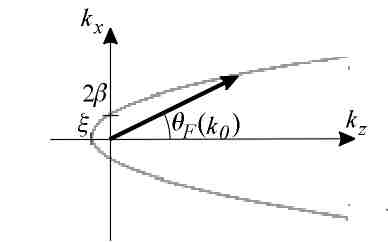
Figure 1: On the geometrical interpretation of the parameters $\beta$ and $\xi$ of the supports of angular spectrum of plane waves of FWM’s (gray line).

The condition

$$v^{g}=c\frac{dk}{dk_{z}}=\left[\frac{1}{c}\frac{d}{dk}\left(k\cos\theta_{F}\left(k\right)\right)\right]^{-1}=\frac{c}{\gamma}\text{,}$$ (32)

where constant $\gamma$ determines the group velocity, yields

$$k_{z}=\gamma k-2\beta\gamma\text{,}$$ (33)

where the integration constant $2\beta$ is defined as the wave number of the plane wave component propagating perpendicularly to the $z$ axis, i.e., $\theta_{F}\left(2\beta\right)=90{{}^{\circ}}$ (see Fig. 1 for the geometrical interpretation of the parameter $\beta$ in $k$-space, the choice is consistent with fw14 ; fw18 for example). Thus, we can write

$$\cos\theta_{F}\left(k\right)=\frac{\gamma\left(k-2\beta\right)}{k}$$ (34)

or

$$k_{F}\left(\theta\right)=\frac{2\beta\gamma}{\gamma-\cos\theta}\text{.}$$ (35)

It appears in section III.1.3 that for a subclass of special cases the above definitions are not appropriate as the corresponding supports of the angular spectrum of plane waves do not intersect with the $k_{x}$ axis. Then one should determine an alternate integration constant $\xi$ from the condition $\theta_{F}\left(\xi\right)=180{{}^{\circ}}$, this choice yields

$$k_{z}\left(k\right)=\left\{\begin{array}[c]{c}\gamma k-\xi\left(\gamma+1\right),~{}\text{if}\mathrm{~{}}\xi\geq 0\\ \gamma k-\xi\left(\gamma-1\right),~{}\text{if}\mathrm{~{}}\xi<0\end{array}\right.$$ (36)

(see Fig. 1 for the geometrical interpretation of the parameter $\xi$ in $k$-space). Thus, we can write

$$\cos\theta_{F}\left(k\right)=\frac{\gamma k-\xi\left(\gamma\pm 1\right)}{k}$$ (37)

or

$$k_{F}\left(\theta\right)=\frac{\xi\left(\gamma\pm 1\right)}{\gamma-\cos\theta}$$ (38)

 so that

$$2\beta=\xi\frac{\gamma+1}{\gamma}$$ (39)

(as we always have $\beta\geq 0$).

The definitions (34) or (35) give the angular spectrum of plane waves in Eq. (31) the form

$$A_{n}^{\left(F\right)}\left(k,\theta\right)=B_{n}\left(k\right)\delta\left[\theta-\theta_{F}\left(k\right)\right]$$ (40)

and

$$A_{n}^{\left(F\right)}\left(k,\theta\right)=B_{n}\left[\theta_{F}\left(k\right)\right]\delta\left[k-k_{F}\left(\theta\right)\right]\text{,}$$ (41)

correspondingly (see Fig. 2 of the section III.1.3 for the set of special cases).

As $k_{z}=k\cos\theta$, our result (40) is consistent with the support of angular spectrum of plane waves of the original FWM’s in Eq. (30), the constant $\gamma$ just generalizes to include also FWM’s of different group velocities. Thus, we can conclude that the physically transparent condition (32) indeed determines the support of the angular spectrum of plane waves of the FWM’s.

III.1.2 Integral expressions for the field of the scalar FWM’s

With the angular spectrum of plane waves (40) we can eliminate variable $\theta$ in integral (31) and get

$$\Psi_{F}\left(\rho,z,\varphi,t\right)=\sum_{n=0}^{\infty}\exp\left[\pm in\varphi\right]\int_{0}^{\infty}\mathrm{d}k\,k^{2}\sin\theta_{F}\left(k\right)$$

$$\qquad\times B_{n}\left(k\right)J_{n}\left[k\rho\sin\theta_{F}\left(k\right)\right]\exp\left[ik\left(z\cos\theta_{F}\left(k\right)-ct\right)\right]\text{~{},}$$ (42)

using (34) we can write

$$\Psi_{F}\left(\rho,z,\varphi,t\right)=\exp\left[-i2\gamma\beta z\right]\sum_{n=0}^{\infty}\exp\left[\pm in\varphi\right]\int_{0}^{\infty}\mathrm{d}k\,k^{2}\sin\theta_{F}\left(k\right)$$

$$\qquad\times B_{n}\left(k\right)J_{n}\left[k\rho\sqrt{1-\left(\frac{\gamma\left(k-2\beta\right)}{k}\right)^{2}}\right]\exp\left[ik\left(\gamma z-ct\right)\right]\text{.}$$ (43)

Alternatively, we can eliminate $k$ by means of Eqs. (41) and get

$$\Psi_{F}\left(\rho,z,\varphi,t\right)=\sum_{n=0}^{\infty}\exp\left[\pm in\varphi\right]\int_{0}^{\pi}\mathrm{d}\theta\,\sin\theta~{}k_{F}^{2}\left(\theta\right)$$

$$\qquad\times B_{n}\left[\theta_{F}\left(k\right)\right]J_{n}\left[k_{F}\left(\theta\right)\rho\sin\theta\right]\exp\left[ik_{F}\left(\theta\right)\left(z\cos\theta-ct\right)\right]\text{~{},}$$ (44)

again (34) transform the equation to

$$\Psi_{F}\left(\rho,z,\varphi,t\right)=\sum_{n=0}^{\infty}\exp\left[\pm in\varphi\right]\int_{0}^{\pi}\mathrm{d}\theta\,\left(\frac{2\beta\gamma}{\gamma-\cos\theta}\right)^{2}\sin\theta$$

$$\qquad\times B_{n}\left[\theta_{F}\left(k\right)\right]J_{n}\left[\frac{2\beta\gamma\rho\sin\theta}{\gamma-\cos\theta}\right]\exp\left[i\frac{2\beta\gamma}{\gamma-\cos\theta}\left(z\cos\theta-ct\right)\right]$$ (45)

[note that analogous expressions can be written using Eqs. (36) – (38)].

The applied condition (32) implies that the longitudinal shape of the central peak of the pulsed wave field in Eqs. (42) – (45) do not spread as it propagates in $z$ axis direction. From the integral expressions it is also obvious that the pulse do not spread in transversal direction. However, the wave field has what has been called the ”local variations” – the term $\exp\left[-i2\gamma\beta z\right]$ in (43) implies that only the instantaneous intensity of the wave field is independent of the propagation distance, in what follows we refer to such wave fields as propagation-invariant.

It is important to note that in Eqs. (40), (41) and (42) – (45) the frequency spectrum is arbitrary. Thus, the necessary and sufficient condition for the propagation-invariance of the general pulsed wave field (31) is that its support of angular spectrum of plane waves should be defined by Eq. (34) or (37). The statement can also be inverted and one can say that the wave field is strictly propagation-invariant only if its support of angular spectrum of plane waves is defined by Eq. (40) or (41) – indeed, in Eq. (32) any other choice would lead to the group velocity dispersion and the pulse would inevitably spread as it propagates. This also implies, that all the possible solutions of scalar homogeneous wave equation that have extended depth of propagation as compared to ordinary Gaussian pulses (see next chapter) should be considered as certain approximations to the FWM’s.

Now, the closed-form expressions like (29) are very convenient in numerical analysis, however, limiting ourselves to the set of available closed-form integrals of (42) – (45) is not reasonable by any means. In this review we use the term ”focus wave modes” (FWM) for all the wave fields that can be represented by the integral expressions (42) – (45), whereas the closed-form expression (29) will be called the original FWM.

III.1.3 A physical classification of FWM’s

The recognition, that the spatiotemporal behavior of FWM’s is determined only by the support of their angular spectrum of plane waves enables one to give a straightforward general classification to the FWM’s.

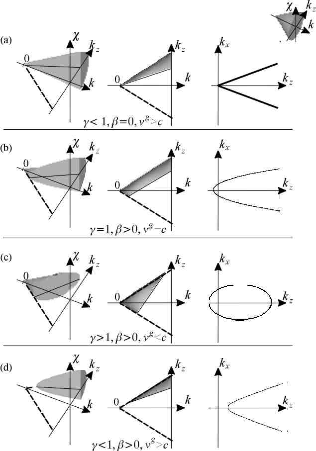
Figure 2: The physical classification of the FWM’s in terms of sections of the cone $\chi^{2}+k_{z}^{2}-k^{2}=0$ in $\left(\chi,k_{z},k\right)$ space. The first two columns depict the sections of the cone from two viewpoints, the corresponding supports of angular spectrums of plane waves are depicted in third column.

Note, the dispersion relation

$$\chi^{2}+k_{z}^{2}-\left(\frac{\omega}{c}\right)^{2}=0$$ (46)

can be interpreted as a definition of a cone in ($\chi,k_{z},k$) space fw15 (see Fig. 2). In this context the specific supports of the angular spectrum of plane waves of FWM’s in Eqs. (32) – (38) have a geometrical interpretation as being the cone sections of (46) along the planes

$$k_{z}=\gamma k-2\beta\gamma$$ (47)

(33) or

$$k_{z}\left(k\right)=\gamma k-\xi\left(\gamma\pm 1\right)$$ (48)

(36). It can be seen that the possible supports of the angular spectrums of plane waves can be divided into four explicit special cases (see Fig. 2) that can be taken as the natural classification of the FWM’s:

• $\beta=0$ ($\xi=0$), $\gamma\leq 1$, the support is a cone in $k$-space, typical examples are Bessel-X pulse and X-pulse (the case $\gamma=1$ corresponds to plane wave pulse);

• $\beta\neq 0$ ($\xi\neq 0$), $\gamma=1$, the support is a paraboloid in $k$-space, typical example is FWM’s, propagating at velocity of light;

• $\beta\neq 0$ ($\xi\neq 0$), $\gamma>1$, the support is an ellipsoid in $k$-space, the group velocity of the FWM’s satisfies $v^{g}<c$;

• $\beta\neq 0$ ($\xi\neq 0$), $\gamma<1$, the support is hyperboloid in $k$-space, the group velocity of the FWM’s satisfies $v^{g}>c$;

Thus, there is barely four general types of strictly propagation-invariant solutions of the scalar wave equation. This point has to be stressed as the straightforward basic idea we set forward here is often elusive in the general literature and numerous closed form LW’s have been set forward.

Pulsed localized wave fields in dispersive media

It should be noted at this point that, in principle, the approach can be used to derive propagation-invariant wave fields for linear dispersive media. In this case we should replace $k_{z}$ by $k_{z}n\left(\omega\right)$ in Eqs. (32) – (35), $n\left(\omega\right)$ being the refractive index of the medium. This modification yields the following equation for the support of the angular spectrum of plane waves of the FWM in linear dispersive media:

$$\tilde{\theta}_{F}\left(\frac{\omega}{c}\right)=\arccos\left[\frac{\gamma\left(\frac{\omega}{c}-2\beta\right)}{n\left(\omega\right)\,\frac{\omega}{c}}\right]\text{,}$$ (49)

$c$ being the velocity of light in vacuum. Eq. (49) defines the support of angular spectrum of plane waves to the wave field that propagates without any longitudinal or transversal spread in linear dispersive media. This approach – to use predetermined angular dispersion to suppress the longitudinal (and transversal) dispersion, though differently formulated, has been already used in Refs. bx2 ; bx5 ; ti20 for example.

III.1.4 The temporal evolution of the FWM’s in the radial direction

The temporal evolution of the FWM’s in the radial direction can be given a convenient mathematical interpretation. Namely, as Chávez-Cerda et al noted in Ref. b16 the monochromatic Bessel beam can be represented as a superposition of so-called Hankel waves

$$\Psi_{m}^{\left(1\right)}\left(\rho,z,t\right) =H_{m}^{\left(1\right)}\left(\chi\rho\right)\exp\left[ik_{z}z-i\omega t+im\varphi\right]$$ (50a)

$$\Psi_{m}^{\left(2\right)}\left(\rho,z,t\right) =H_{m}^{\left(2\right)}\left(\chi\rho\right)\exp\left[ik_{z}z-i\omega t+im\varphi\right]\text{,}$$ (50b)

where

$$H_{m}^{\left(1\right)}\left(\chi\rho\right) =J_{m}\left(\chi\rho\right)+iN_{m}\left(\chi\rho\right)$$ (51a)

$$H_{m}^{\left(2\right)}\left(\chi\rho\right) =J_{m}\left(\chi\rho\right)-iN_{m}\left(\chi\rho\right)$$ (51b)

are the m-th order Hankel functions and $$N_{m} xy$$ denotes the m-th order Neumann function (the Bessel function of the second kind). For monochromatic wave fields the two solutions define the diverging and converging wave in plane, in other terms, they form the ”sink” and ”source” pair. In those terms the m-th order Bessel beam can be written as

$$J_{m}\left(\chi\rho\right)\exp\left[ik_{z}z-i\omega t+im\varphi\right]=$$ (52)

$$\qquad\qquad\qquad\left[H_{m}^{\left(1\right)}\left(\chi\rho\right)+H_{m}^{\left(2\right)}\left(\chi\rho\right)\right]\exp\left[ik_{z}z-i\omega t+im\varphi\right]$$

– this is a standing wave that arise in the superposition of the two Hankel waves (note how the singularity of the Neumann functions at the origin is eliminated).

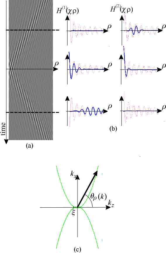
Figure 3: (a) Typical spatiotemporal field distribution of a FWM; (b) The temporal evolution of the FWM in radial direction as the superposition of the pulsed Hankel beams (blue solid lines), the amplitude of the corresponding carrier-frequency monochromatic Hankel beam is added for comparison (red dotted line); (c) The support of the angular spectrum of plane waves of a wave field that is propagation-invariant in radial direction (see text).

This approach can be easily generalized for the wideband wave fields – in this case the superposition of the monochromatic Hankel beams form a converging or expanding circular pulse in the $xy$ plane. If we also use condition (40) we get the pulse that corresponds to the radial evolution of the FWM’s. The results of a numerical simulation of its behavior are depicted in Fig. 3a and 3b.

Note also, that the radial wave that propagates away from the $z$ axis is generally not propagation invariant. Indeed, if we follow the arguments of the section III.1.1 for radial propagation we can write the condition of propagation-invariance as

$$v^{g}=c\frac{dk}{d\chi}=\left[\frac{1}{c}\frac{d}{dk}\left(k\sin\theta_{F}^{\left(\rho\right)}\left(k\right)\right)\right]^{-1}=\frac{c}{\gamma_{\rho}}\text{,}$$ (53)

where constant $\gamma_{\rho}$ again determines the group velocity. Specifying the integration constant $\xi$ again from the condition $\theta_{\rho}\left(\xi\right)=180{{}^{\circ}}$ we can write for the support of angular spectrum of plane waves

$$k\sin\theta_{F}^{\left(\rho\right)}\left(k\right)=\gamma_{\rho}k-\xi\left(\gamma_{\rho}+1\right)\text{.}$$ (54)

Thus, we can write

$$\sin\theta_{F}^{\left(\rho\right)}\left(k\right)=\frac{\gamma_{\rho}k-\xi\left(\gamma_{\rho}+1\right)}{k}$$ (55)

(note that in this context $\xi\geq 0$).

A typical support of the angular spectrum of plane waves defined by Eq. (54) is depicted in Fig. 3b. So, the FWM is propagation-invariant in both the $z$ axis direction and radial direction only in the special case $\xi\equiv 0$ where we can write $\gamma_{\rho}=\sqrt{1-\gamma^{2}}$. This consequence will be given a further interpretation in section III.3.1.

III.1.5 The spatial localization of FWM’s

For most practical cases there is no closed-form integrals to Eq. (42). Consequently, we have to deal with integral transforms and the straightforward numerical simulation of any realistic situation may be a tedious task (this is especially true for general LW’s where the double integrals have to be computed). However, for LW’s there is a simple method for qualitative estimate of the resulting wave fields, based on three-dimensional Fourier transforms (the monochromatic case of the approach was introduced by McCutchen in Ref. mc5 and has been used for example in Refs. mc10 ; mc15 ).

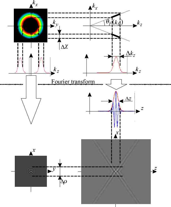
Figure 4: The Fourier transform estimation of the spatial shape of the FWS’s (see text).

Let us start with Whittaker type plane wave decomposition in Eq. (13) and set $t=0$:

$$\Psi^{\prime}\left(x,y,z,0\right)=\int\int\int_{-\infty}^{\infty}\mathrm{d}k_{x}\mathrm{d}k_{y}\mathrm{d}k_{z}$$

$$\qquad\qquad\times A\left(k_{x},k_{y,}k_{z}\right)\exp\left[i\left(k_{x}x+k_{y}y+k_{z}z\right)\right]\text{.}$$ (56)

Obviously we can write for the field on $z$ axis the relation

$$\Psi^{\prime}\left(0,0,z,0\right)=\int_{-\infty}^{\infty}\mathrm{d}k_{z}\exp\left[ik_{z}z\right]\left\{\int\int_{-\infty}^{\infty}\mathrm{d}k_{x}\mathrm{d}k_{y}A\left(k_{x},k_{y,}k_{z}\right)\right\}\text{,}$$ (57)

so that

$$\Psi^{\prime}\left(0,0,z,0\right)=\int_{-\infty}^{\infty}\mathrm{d}k_{z}\exp\left[ik_{z}z\right]A_{xy}\left(k_{z}\right)\text{,}$$ (58)

where

$$A_{xy}\left(k_{z}\right)=\int\int_{-\infty}^{\infty}\mathrm{d}k_{x}\mathrm{d}k_{y}A\left(k_{x},k_{y,}k_{z}\right)$$ (59)

and from the definition of one-dimensional Fourier transform, we can write

$$\Psi^{\prime}\left(0,0,z,0\right)=2\pi\mathcal{F}_{z}^{-1}\left[A_{xy}\left(k_{z}\right)\right]\text{.}$$ (60)

Here $\mathcal{F}_{z}^{-1}\left[...\right]$ denotes the inverse Fourier’ transform in $k_{z}$-direction and the integral (59) can be thought of as the projection of the angular spectrum plane waves onto the $z$ axis (see Fig. 4). Similarly we can write for the filed in $xy$ plane at $z=0$

$$\Psi^{\prime}\left(x,y,0,0\right) =\int\int_{-\infty}^{\infty}\mathrm{d}k_{x}\mathrm{d}k_{y}\exp\left[ik_{x}x+ik_{y}y\right]$$

$$\times\left\{\int_{-\infty}^{\infty}\mathrm{d}k_{z}A\left(k_{x},k_{y,}k_{z}\right)\right\}\text{,}$$ (61)

so that

$$\Psi^{\prime}\left(x,y,0,0\right)=\left(2\pi\right)^{2}\mathcal{F}_{xy}^{-1}\left[A_{z}\left(k_{x},k_{y}\right)\right]\text{,}$$ (62)

where

$$A_{z}\left(k_{x},k_{y}\right)=\int_{-\infty}^{\infty}\mathrm{d}k_{z}A\left(k_{x},k_{y,}k_{z}\right)$$ (63)

and $\mathcal{F}_{xy}^{-1}\left[...\right]$ denotes the two-dimensional inverse Fourier transform.

Now, having in mind the table of basic one- and two-dimensional Fourier transforms and the general properties of Fourier transforms, the knowledge of the defined projections of angular spectrum of plane waves onto the $k_{z}$ axis and $k_{x}k_{y}$ plane allows one immediately estimate the general shape of the wave field on $z$ axis and $xy$ plane respectively. If we also note that in studies of the propagation-invariant wave fields the estimates are valid over the entire $z$ axis (for space-time points $\gamma z-ct$), the approach can prove to be very useful.

Let us specify the frequency spectrum of the light source $\emph{s}\left(k\right)$ as the Gaussian one:

$$\emph{s}\left(k\right)=\exp\left[-\frac{1}{2}\sigma_{k}^{2}\left(k-k_{0}\right)^{2}\right]\text{,}$$ (64)

where $k_{0}$ denote the mean wave number of the wave field and $\sigma_{k}$ is determined from the pulse length $\tau_{s}$ of the corresponding plane wave pulse as

$$\sigma_{k}=\frac{c\tau_{s}}{2\sqrt{2\ln 2}}\text{.}$$ (65)

From the known character of the angular spectrum of plane waves of the FWM’s we can approximate for the Gaussian profiles of the $k_{z}$ and $\chi$ projections of the angular spectrum of plane waves

$$\sigma_{z} =\frac{\sigma_{k}}{\cos\theta_{F}\left(k_{0}\right)}$$ (66a)

$$\sigma_{\rho} =\frac{\sigma_{k}}{\sin\theta_{F}\left(k_{0}\right)}$$ (66b)

respectively.

The spectral profile of the $k_{z}$-projection of the angular spectrum of plane waves then reads

$$A_{xy}\left(k_{z}\right)\propto\exp\left[-\frac{1}{2}\sigma_{z}^{2}\left(k_{z}-k_{z0}\right)^{2}\right]$$ (67)

with the FWHM (full width at half-maximum)

$$\Delta k_{z}\approx\Delta k\cos\theta_{F}\left(k_{0}\right)=\frac{2\sqrt{2\ln 2}}{\sigma_{z}}\text{,}$$ (68)

where

$$\Delta k=\frac{2\sqrt{2\ln 2}}{\sigma_{k}}\text{.}$$ (69)

The corresponding intensity profile is

$$\mathcal{F}_{z}^{-1}\left[A_{xy}\left(k_{z}\right)\right]\propto\exp\left[-\frac{z^{2}}{2\sigma_{z}^{2}}\right]$$ (70)

with FWHM

$$\Delta z\approx\frac{c\tau_{s}}{\cos\theta_{F}\left(k_{0}\right)}=\sigma_{z}2\sqrt{2\ln 2}\text{.}$$ (71)

For the field in transversal direction we can give a good estimate by recognizing that the intensity profile on $xy$ plane has the Bessel profile that is multiplied by an envelope. The profile of the latter can be estimated by the 1D Fourier transform of the projection of the angular spectrum along an axis and we can write

$$A_{z}\left(k_{x},k_{y}\right)\propto\exp\left[-\frac{1}{2}\sigma_{\rho}^{2}\left(\chi-\chi_{0}\right)^{2}\right]\text{,}$$ (72)

with FWHM

$$\Delta\chi\approx\Delta k\sin\theta_{F}\left(k_{0}\right)=\frac{2\sqrt{2\ln 2}}{\sigma_{\rho}}\text{.}$$ (73)

The corresponding intensity profile reads

$$\mathcal{F}_{xy}^{-1}\left[A_{z}\left(k_{x},k_{y}\right)\right]\propto J_{0}\left(k\rho\sin\theta_{F}\left(k_{0}\right)\right)\exp\left[-\frac{\rho^{2}}{2\sigma_{\rho}^{2}}\right]$$ (74)

with FWHM

$$\Delta\rho\approx\left\{\begin{array}[c]{c}\sigma_{\rho}2\sqrt{2\ln 2}\text{ -- the envelope\qquad\qquad\qquad\qquad\qquad}\\ \frac{2\times 2.405}{k_{0}\sin\theta_{F}\left(k_{0}\right)}\text{ -- the central peak of the Bessel function}\end{array}\right.$$ (75)

(see Fig. 4 for an illustration of the description). Note, that as we can write the ratio

$$\frac{\sigma_{z}}{\sigma_{\rho}}=\frac{\Delta z}{\Delta\rho}=\tan\theta_{F}\left(k_{0}\right)$$ (76)

for the pulse widths in the two directions, we at once can deduce that for optically feasible FWM’s [$\theta_{F}\left(k_{0}\right)\ll 1$] the central peak is better localized along the $z$ axis.

III.2 Few remarks on properties of FWM’s

III.2.1 Causality of FWM’s

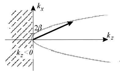
Figure 5: On the causal and acausal components of the angular spectrum of plane waves of FWM’s. The striped region denotes the acausal region of the support of the angular spectrum of plane waves.

In several papers it has been noted, that the original FWM’s introduced by Brittingham and Ziolkowski in Eq. (29) are not exactly causal as they include backward propagating plane wave components (see Fig. 5) fw13a . This fact is due to the specific frequency spectrum (30) that leads to the closed-form FWM’s (see the overview in following chapter). In the consequent publications (see Ref. [fw18 ]) Shaarawi et. al. demonstrated, that the parameters of the spectrum can be chosen so that the predominant part of the energy of the FWM’s is in forward propagating plane wave components.

In the context of our approach this problem has to be considered as ill-posed – as all the wave fields that share the support of the angular spectrum of plane waves (40) are propagation-invariant regardless of their frequency spectrum, we can just choose one without the acausal components.

III.2.2 FWM’s and evanescent waves

The second topic that is closely related to the backward propagating plane wave components of the original FWM’s is the one of evanescent waves fw18 ; fw20 .

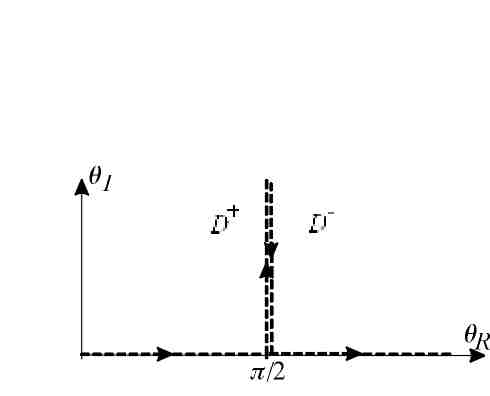
Figure 6: The integration contour in Weyl picture of angular spectrum of plane waves. The vertical part of the contour where the imaginaty part of the angle $\theta$ is nonzero cancels out in integration.

From the practical point of view it may seem peculiar to introduce the evanescent waves, the intensity of which decays exponentially, in the context of the propagation-invariant wave fields where the depth of the propagation usually extend over several meters. However, the evanescent waves appear indeed in a Weyl picture of the FWM’s. Indeed, from Eqs. (21) and (33) one can write

$$A_{n}^{we}\left(k,\chi\right)=B_{n}\left(k\right)\delta\left[k-\sqrt{k^{2}-\chi^{2}}-2\beta\right]$$ (77)

for the angular spectrum of plane waves of the FWM’s so that the field can be written as

$$\Psi\left(\rho,z,\varphi,t\right)=\sum_{n=0}^{\infty}\exp\left[\pm in\varphi\right]\int_{0}^{\infty}\mathrm{d}k\int_{0}^{\infty}\mathrm{d}\chi\chi~{}B_{n}\left(k\right)$$ (78)

$$\qquad\times J_{n}\left(\chi\rho\right)\delta\left[k-\sqrt{k^{2}-\chi^{2}}-2\beta\right]\exp\left[i\left(z\sqrt{k^{2}-\chi^{2}}-ckt\right)\right]\text{.}$$

In Eq. (78), for the ranges $\chi<k$ the integration is over homogeneous plane waves. For $\chi>k$, the wave vector of the plane waves is purely imaginary and the integration is over the evanescent waves fw18 ; lw6 . The situation may be more apparent if we transform to variables $\chi,k\rightarrow\theta,k$ and write (for cylindrically symmetric component only for brevity)

$$\Psi^{\left(\pm\right)}\left(\rho,z,t\right)=\int_{0}^{\infty}\mathrm{d}k~{}k^{2}\int_{D^{\pm}}\mathrm{d}\theta\cos\theta\sin\theta$$ (79)

$$\qquad\times B_{0}\left(k\right)\delta\left[k\mp k\cos\theta-2\beta\right]J_{0}\left(k\rho\sin\theta\right)\exp\left[\pm ikz\cos\theta-i\omega t\right]$$

or

$$\Psi^{\left(\pm\right)}\left(\rho,z,t\right)=\int_{D^{\pm}}\mathrm{d}\theta\frac{2\beta\sin\theta~{}B_{0}\left(\frac{2\beta}{\gamma\left(1-\cos\theta\right)}\right)}{\gamma\left(1-\cos\theta\right)}$$ (80)

$$\qquad\times J_{0}\left(\frac{2\beta\rho\sin\theta}{\gamma\left(1-\cos\theta\right)}\right)\exp\left[\pm i\frac{2\beta}{\gamma\left(1-\cos\theta\right)}\left(z\cos\theta\mp ct\right)\right]\text{.}$$

Here ”$+$” stands for forward propagating plane wave components and ”$-$” stands for backward propagating plane wave components and the integration is carried out along the contours $D^{\pm}$ of complex $\theta$ plane, $\chi/k=\sin\left(\theta_{R}+i\theta_{I}\right)$ (see Fig. 6). Also, if the analysis is carried out for wave fields the angular spectrum of plane waves of which has forward and backward propagating components, the total wave field can be written as fw18

$$\Psi=\left(\Psi_{h}^{+}+\Psi_{ev}^{+}\right)+\left(\Psi_{h}^{-}+\Psi_{ev}^{-}\right)\text{,}$$ (81)

where subscript ”$h$” denotes homogeneous component of $\Psi^{+}$ or $\Psi^{-}$, i.e., $0\leq\theta_{R}\leq 2\pi$, $\theta_{I}=0$ and subscript ”$ev$” denotes evanescent components, i.e., $\theta_{R}=\pi/2$, $\theta_{I}<0$. It has been shown fw18 , that for the evanescent components of a free field one has

$$\Psi_{ev}^{+}=-\Psi_{ev}^{-}\text{,}$$ (82)

so that the Weyl forward and backward propagating components add up resulting in the source-free solution in Eq. (42).

Again, in our approach the frequency spectrum is chosen so that the wave fields do not have any backward propagating components. Consequently, the integration is only along the real part of the $D^{+}$. Also, it is quite clear that for the free-space wave fields the presence of the evanescent waves in the integration (80) is rather a peculiarity of the Weyl type angular spectrum of plane waves. For example, if we write the Weyl picture of a plane wave pulse propagating perpendicularly to $z$ axis, the corresponding Weyl picture obviously do contain evanescent components. However, there is no physical content in those components.

III.2.3 Energy content of scalar FWM’s

As already noted, the total energy content of FWM’s is infinite fw2 ; fw5 ; lw1 . Indeed, as the energy content is calculated as

$$U_{tot}=\int_{-\infty}^{\infty}\mathrm{d}z\int_{0}^{\infty}\mathrm{d}\rho\rho\int_{0}^{2\pi}\mathrm{d}\varphi\left|\Psi_{F}\left(z,\rho,\varphi,t\right)\right|^{2}\text{~{}.}$$ (83)

In the Fourier picture, the Parseval relation and the angular spectrum of plane waves in Eq. (41) can be used to yield

$$U_{tot} =\sum_{n}\int_{0}^{\infty}\mathrm{d}k\int_{0}^{\pi}\mathrm{d}\theta\mathbf{\,}\left|\tilde{B}_{n}\left(k\right)\delta\left[\theta-\theta_{F}\left(k\right)\right]\right|^{2}$$

$$=\sum_{n}\int_{0}^{\infty}\mathrm{d}k\int_{0}^{\pi}\mathrm{d}\theta\mathbf{\,}\left|\tilde{B}_{n}\left(k\right)\right|^{2}\delta^{2}\left[\theta-\theta_{F}\left(k\right)\right]$$ (84)

so that

$$U_{tot}=\infty$$ (85)

due to the $\delta^{2}$ in the integrand (here and hereafter the tilde on angular spectrum indicates that the factor $k^{2}\sin\theta$ is included into the spectrum).Obviously the relation (85) is valid whenever there is a delta function in the definition of the angular spectrum of plane waves. Also, it has been proved that any wave field that is strictly propagation-invariant has necessarily infinite total energy fw3 ; fw3o1 .

The second important energetic parameter of the LW’s is their energy flow over a cross-section per unit time – obviously, any physically feasible wave field has to have a finite energy flow. In terms of the previous section and using the two-dimensional Parseval relation this quantity can be calculated as

$$\Phi_{xy}=\int\int_{-\infty}^{\infty}\mathrm{d}k_{x}\mathrm{d}k_{y}\left|A_{z}\left(k_{x},k_{y}\right)\right|^{2}\text{,}$$ (86)

where $A_{z}\left(k_{x},k_{y}\right)$ is again the projection of the angular spectrum of plane waves onto $k_{x}k_{y}$ plane. Obviously the quantity is necessarily infinite, if only the projection of the angular spectrum can be written in terms of delta function in $k_{x}k_{y}$ plane. Otherwise the energy flow is finite, provided the function $A_{z}\left(k_{x},k_{y}\right)$ is square integrable. The comparison of Figs. 2 and 4 shows that the FWM’s generally have finite total energy flow.

In literature the finite energy LW’s have been constructed for example by means of superpositions of FWM’s fw5 ; lw1 and by applying finite time windows g3 ; g4 ; g5 ; g6 ; g10 . In section. VI.3 we will describe our approach to this problem as described in Ref. m3 .

III.3 Alternate derivations of scalar FWM’s

III.3.1 FWM’s as cylindrically symmetric superpositions of tilted pulses

As to demonstrate the efficiency of the integral transform representations in describing the properties of FWM’s, we give yet another description of FWM’s (Ref. m4 ).

Let us represent FWM’s as the cylindrically symmetric superpositions of the interfering pairs of certain tilted pulses (see also Ref. m1 ). In this representation the field of the FWM’s can be expressed as [see Eqs. (15) and (40)]

$$\Psi_{F}\left(\rho,z,t\right) =\int_{0}^{\pi}\mathrm{d}\phi\left[T\left(x,y,z,t;\phi\right)+T\left(x,y,z,t;\phi+\pi\right)\right]$$ (87)

$$=\int_{0}^{\pi}\mathrm{d}\phi F^{\prime}\left(x,y,z,t;\phi\right)\text{,}$$

where $T\left(x,y,z,t;\phi\right)$ denotes the field of the tilted plane wave pulses, that in the spectral representation are given by

$$T\left(x,y,z,t;\phi\right)=\int_{0}^{\infty}\mathrm{d}k~{}\tilde{A}\left(k,\theta_{F}\left(k\right),\phi\right)$$ (88)

$$\quad\times\exp\left[ik\left(x\cos\phi\sin\theta_{F}\left(k\right)+y\sin\phi\sin\theta_{F}\left(k\right)+z\cos\theta_{F}\left(k\right)-ct\right)\right]\text{,}$$

where $\tilde{A}\left(k,\theta_{F}\left(k\right),\phi\right)$ is the angular spectrum of plane waves of the wave field and the angular function $\theta_{F}\left(k\right)$ is defined by Eq. (34). From Eqs. (87) and (88) we get

$$F^{\prime}\left(x,y,z,t;\phi\right)=2\int_{0}^{\infty}\mathrm{d}k~{}\tilde{A}\left(k,\theta_{F}\left(k\right),\phi\right)$$ (89)

$$\qquad\times\cos\left[k\sin\theta_{F}\left(k\right)\left(x\cos\phi+y\sin\phi\right)\right]\exp\left[ik\left(z\cos\theta_{F}\left(k\right)-ct\right)\right]\text{.}$$

An example of a tilted pulse with Gaussian frequency spectrum corresponding to approximately $\tau_{s}\sim 4fs$ in Eq. (88) is depicted in Fig. 7a, the corresponding superposition of two tilted pulses in Eq. (89) and FWM in Eq. (42) are depicted in Fig. 7b).

In this representation the properties of FWM’s can be given the following interpretation:

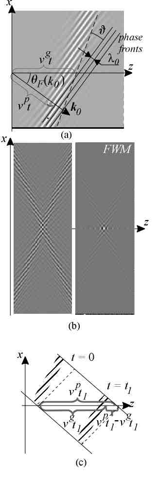
Figure 7: (a) On the field distribution of tilted pulses; (b) comparison of field of the superposition of a pair of tilted pulses (in left) and of the corresponding FWM (in right); (c) on the difference of phase and group velocities of the FWM’s (see text).

• The localized central peak of FWM’s is simply the well-known consequence of taking the axially symmetric superposition of a harmonic function. Indeed, the interference of the two transform-limited tilted pulses in Eq. (89) gives rise to the harmonic interference pattern, the transversal width of which is proportional to the temporal length of the tilted pulses (88). The central peak arises due to the constructive interference of the tilted pulses along the optical axis, formally, the $\cos\left({}\right)$ function in Eq. (89) is replaced by $J_{0}\left({}\right)$ in Eq. (42) [see Fig. 7b];

• The nondispersing propagation of the optical FWM’s wave fields can be given an alternate wave-optical interpretation. Namely, it can be seen from Fig. 8, that in large scale the longitudinal length of the tilted pulses depends on the distance from the optical axis so that the tilted pulses have a ”waist” (this claim is identical to that given in section III.1.4 that the radial wave propagating toward the $z$ axis and back is not propagation-invariant). The relation (34) essentially guarantees, that the waist propagates along the optical axis and do not spread – in this case the central peak of the corresponding cylindrically symmetric superpositions, FWM’s (42), also remains transform-limited;

  

  Figure 8: The large-scale behaviour of the spatial shape of the modulus of the tilted pulses.

• The local variations of the central peak of the wave field, noted for example in Ref. fw5 , can be explained as the result of the difference between the phase and group velocities along the optical axis – as can be seen from Fig. 7c the pulse and phase fronts of the tilted pulses are not parallel;

• The group velocity of the wave field can be set by changing the parameter $\gamma$ in Eq. (34). The Fig. 7c gives this effect a wave optical interpretation – it can be seen, that the on-axis group velocity of the wave field directly depends on the angle between the phase front and pulse front and on the direction of the wave vector of the mean frequency.

It is easy to see, that all the presented arguments are equally valid for the superpositions of tilted pulses in Eq. (89) and for its cylindrically symmetric counterparts – FWM’s. Thus, we can state that the defined interfering pair of tilted pulses possess all the characteristic properties of FWM’s. In fact, the physics behind the two wave fields is similar to the degree, that we will call the wave field (89)

$$F\left(x,z,t\right)=\int_{0}^{\infty}\mathrm{d}k~{}\tilde{B}_{0}\left(k\right)\cos\left[kx\sin\theta_{F}\left(k\right)\right]\exp\left[ik\left(z\cos\theta_{F}\left(k\right)-ct\right)\right]$$ (90)

as two-dimensional FWM (2D FWM) in what follows.

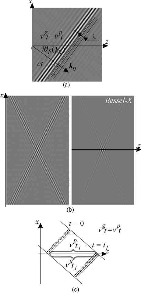
Figure 9: (a) On the phase and group velocity of a plane wave pulse propagating at angle $\theta_{0}$ relative to $z$-axis; (b) comparison of the field of the superposition of a pair of plane wave pulses (in left) and of their corresponding cylindrically symmetric superposition – Bessel-X pulse (in right); (c) on the group velocity of Bessel-X pulses.

We end this section by noting that the special case of this approach can be used to discuss the properties of X-type pulses (Ref. m1 ). In this case $\theta_{F}\left(k\right)=const=\theta_{0}$ and we have the interference of two plane wave pulses:

$$T\left(x,y,z,t;\phi\right) =\int_{0}^{\infty}\mathrm{d}k~{}\tilde{A}\left(k,\theta_{F}\left(k\right),\phi\right)$$ (91)

$$\times\exp\left[ik\left(x\cos\phi\sin\theta_{0}y\sin\phi\sin\theta_{0}+z\cos\theta_{0}-ct\right)\right]\text{,}$$

so that

$$F\left(x,z,t\right)=\int_{0}^{\infty}\mathrm{d}k~{}\tilde{B}_{0}\left(k\right)\cos\left[kx\sin\theta_{0}\right]\exp\left[ik\left(z\cos\theta_{0}-ct\right)\right]\text{.}$$ (92)

(see Fig. 9)

III.3.2 FWM’s as the moving, modulated Gaussian beams

In literature the closed-form expression (29) for the original FWM’s have been derived with the use of the anzatz fw3 ; fw4 ; fw5

$$\Psi\left(x,y,z,t\right)=\exp\left[i\beta\mu\right]F^{\prime}\left(x,y,\zeta\right)\text{~{},}$$ (93)

where $\mu=z+ct$ and $\zeta=z-ct$. With (93) the wave equation (8) reduces to the Schrödinger equation for $F^{\prime}$

$$\left(\Delta_{\bot}+4i\beta\partial_{\zeta}\right)F^{\prime}\left(x,y,\zeta\right)=0$$ (94)

which, assuming axial symmetry, has a solution of the form fw5

$$F^{\prime}\left(\rho,\zeta\right)=\frac{1}{4\pi i\left(a_{1}+i\zeta\right)}\exp\left[-\frac{\beta\rho^{2}}{a_{1}+i\zeta}\right]\text{,}$$ (95)

so that one can write the solution similar to the FWM’s in Eq. (29)

$$\Psi_{f}\left(\rho,\mu,\zeta\right)=\exp\left[i\beta\mu\right]\frac{a_{1}}{4\pi i\left(a_{1}+i\zeta\right)}\exp\left[-\frac{\beta\rho^{2}}{a_{1}+i\zeta}\right]\text{~{}.}$$ (96)

To give the FWM a more convenient form one can use the transform

$$\frac{1}{a_{1}+i\zeta}=\frac{1}{\beta a_{1}^{2}\left(\zeta\right)}-i\frac{1}{R\left(\zeta\right)}$$ (97)

with which the Eq. (96) can be shown to yield

$$\Psi_{f}\left(\rho,z,\zeta\right)=\frac{W_{0}}{4\pi a_{1}\left(\zeta\right)}\exp\left[-i\beta\zeta\right]$$ (98)

$$\qquad\times\exp\left[-\frac{\rho^{2}}{a_{1}^{2}\left(\zeta\right)}+i\frac{\beta\rho^{2}}{R\left(\zeta\right)}-i\left(\arctan\left(\frac{\zeta}{a_{1}}\right)-2\beta z\right)\right]\text{,}$$

where

$$a_{1}\left(\zeta\right) =W_{0}\left[1+\left(\frac{\zeta}{a_{1}}\right)^{2}\right]^{\frac{1}{2}}$$ (99a)

$$R\left(\zeta\right) =\zeta\left[1+\left(\frac{a_{1}}{\zeta}\right)^{2}\right]$$ (99b)

and

$$W_{0}=\sqrt{\frac{a_{1}}{\beta}}~{}\text{.}$$ (100)

If one compares the Eqs. (98) - (100) to those of the monochromatic Gaussian beam (see Ref. o25 for example) one can see that, the FWM’s can be interpreted as moving, modulated Gaussian beams for which $a_{1}\left(\zeta\right)$ and $R\left(\zeta\right)$ are the beam width and radius of curvature respectively and $W_{0}$ is the beam waist at $\zeta=0$ (see Refs. fw3 ; fw4 ; fw5 for relevant descriptions).

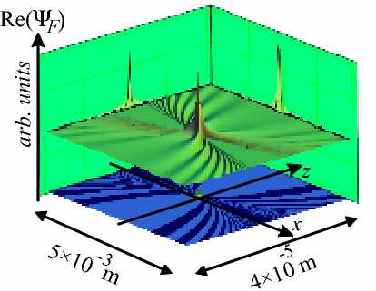
Figure 10: A numerical example of the field of the original FWM’s.

Now, several interesting consequences can be drawn at this point. Most importantly, this formal analogy between the FWM’s and Gaussian beams is very conditional and even misleading in some respects. First of all, the constant $\beta$ is by no means the carrier wave number of the FWM’s as one might expect from the corresponding monochromatic expression – in the following Chapter IV we will see that the convenient choice of parameter for optically feasible FWM’s with the carrier wave number $k_{0}\approx 1\times 10^{7}\frac{rad}{m}$ the parameter is of the order of magnitude $\beta\lesssim 100\frac{rad}{m}$. Secondly, the requirement of optical feasibility also implies that $a_{1}\ll 1$ (see Sec. IV.2) and with this condition the original FWM’s (see Fig. 10) typically do not resemble that of the Gaussian beam as they appear in the textbook examples. The reason for the ”abnormal” behaviour is obvious – with the above conditions the direct analogy to the monochromatic case, where $\beta=2\pi/\lambda$, yields for the beam waist in Eq. (100) $W_{0}\ll\lambda$. So that we have a limiting case where the waist of the Gaussian beam is much less than its wavelength – clearly here the different physical nature of the FWM’s show up.

Next we would like to discuss the claim, often encountered in literature, that the original FWM’s are carrier free wave fields. First of all, in lights of the general physical considerations in section III.1.5 it should be evident that the non-oscillating shape of the central peak in Fig. 10 is a direct consequence of the ultra-wide frequency spectrum of the wave field – if the pulse length of the corresponding source plane wave pulse is less than the central wavelength, the resulting FWM is effectively an half-cycle pulse and in this condition the concept of carrier wavelength is rather meaningless of course. However, in above sections it was shown that the general FWM’s are not confined to the one particular frequency spectrum. Correspondingly, we can choose a feasible frequency spectrum and the carrier free behaviour of the original FWM’s should certainly not be mentioned as the defining property of the original FWM’s, this is just a mathematical peculiarity of a particular integral transform table entry.

Figure 11: On the character of the Gouy phase shift term in the closed form expression of the FWM’s: The real part of the original FWM (dotted blue line) is depicted for three $z$-coordinate values together with the modulus (solid green line) and real part (solid black line) of an FWM with narrower bandwidth (see text).

The issue can be given an alternate description if we note that, using the analogy to the monochromatic Gaussian beams the term

$$G\left(z,\zeta\right)=i\left(\arctan\left(\frac{\zeta}{a_{1}}\right)+2\beta z\right)$$ (101)

in the expression Eq. (98) could be interpreted as the Gouy phase shift [o25 ] of the FWM’s. In previous section III.3.1 we described the FWM’s as the cylindrically symmetric superpositions of certain tilted pulses. Now, the original FWM’s differ from those, depicted in Fig. 7b only by the ultra-wide bandwidths. In Fig. (11) we have depicted the on-axis spatial evolution of an FWM as described by Eq. (98) and of one of reasonable bandwidth, calculated from the Eq. (42). The comparison of the two waveforms shows that term $\exp\left[i\arctan\left(\frac{\zeta}{a_{1}}\right)\right]$ of the phase term $G$ can be interpreted as the remnants of the sinusoidal waveform, lost due to the ultra-wide bandwidth and the term $\exp\left[i2\beta z\right]$ is added as the monothonically growing phase factor that is due to the difference between the group and phase velocities of FWM’s. The latter term is characteristic to the FWM’s only – instead of having a single focus with accompanying Gouy phase shift or a ”frozen” Gouy phase shift as the X-type pulses, FWM’s have periodically evolving phase shift term.

The idea of Gouy phase shift, initially introduced in the Fresnel approximation of the diffraction theory of monochromatic focused beams, has attracted a renewed interest recently in the context of propagation of subcycle Gaussian pulses (see Refs. ve35 ; go15 ; go20 ; go25 ; go30 ; go35 ; go40 ). We believe, that the simple physical interpretation of the term (101) in the context of FWM’s, as being the result of the difference between phase and group velocities of the wave field, might add to the general understanding of the phenomenon.

III.3.3 FWM’s as the Lorentz transforms of focused monochromatic beams

An interesting interpretation to the FWM’s can be given in terms of special theory of relativity. Namely, in Ref. fw4 Bélanger demonstrated that Gaussian monochromatic beams appear as FWM’s (Gaussian packetlike beams) when observed in an inertial system moving at relativistic speeds relative to the focused wave. In this short note we would like to give an another mathematical representation to this claim.

Suppose we take a focused monochromatic wave of the form

$$\Psi\left(\rho,z,t\right)=\int_{0}^{\pi}d\theta K\left(\theta\right)\exp\left[ik_{0}\left(z\cos\theta-ct\right)\right]$$ (102)

with angular spectrum of plane waves

$$A_{0}\left(k,\theta\right)=K\left(\theta\right)\delta\left(k-k_{0}\right)\text{.}$$ (103)

If we observe the beam from a moving inertial system, the plane wave components of the field suffer from the relativistic Doppler shift. As the result, their wave vectors and frequencies transform as described by Lorentz transformations. Specifically, the wave number of the wave vector and its longitudinal and transversal components in the inertial frame, moving at speed $V$ along the $z$ axis, obey equations

$$k^{\prime} =\gamma_{l}k_{0}\left(1-\beta_{l}\cos\theta\right)$$ (104a)

$$k_{z}^{\prime} =\gamma_{l}k_{0}\left(\cos\theta-\beta_{l}\right)$$ (104b)

$$k_{x}^{\prime} =k_{0}\sin\theta=k_{x}$$ (104c)

$$k_{y}^{\prime} =k_{0}\sin\theta=k_{y}$$ (104d)

(Eq. (11.29) of Ref. o15 ) where $$k_{0}$$ is the wave number of the wave field in rest frame and

$$\beta_{l}\left(V\right) =\frac{V}{c}$$ (105a)

$$\gamma_{l}\left(V\right) =\frac{1}{\sqrt{1-\beta^{2}}}$$ (105b)

We can use Eq. (104a) to eliminate $$\theta$$ from Eq. (104b) to get

$$k_{z}^{\prime}=-\frac{1}{\beta_{l}\left(V\right)}k^{\prime}-\gamma_{l}\left(V\right)k_{0}\left(\beta_{l}\left(V\right)-\frac{1}{\beta_{l}\left(V\right)}\right)$$ (106)

and if we define the parameters as

$$\gamma\left(V\right) =\frac{1}{\beta_{l}\left(V\right)}$$ (107a)

$$\beta\left(V,k_{0}\right) =\frac{\gamma_{l}\left(V\right)k_{0}}{2}\text{~{},}$$ (107b)

we can write for the $$z$$ component of the wave vector

$$k_{z}^{\prime}=-\gamma\left(V\right)k^{\prime}-2\beta\left(V,k_{0}\right)\left(\frac{1}{\gamma\left(V\right)}-\gamma\left(V\right)\right)\text{.}$$ (108)

Thus, if the velocity of the moving frame is close to the speed of light, the angular spectrum of plane waves of the wave field in the moving frame is the one of the FWM that moves in negative direction of $z$ axis – for the FWM’s we have in Eq. (33)

$$k_{z}=\gamma k-2\beta\gamma$$ (109)

and using both $k_{0}$ and $V$ as parameters we can model every possible support of angular spectrum of plane waves of FWM’s. In Fig. 12 the support of angular spectrum of plane waves of the beam as seen from the moving reference system is depicted for various values of the speed $V$ and fixed value for $k_{0}$.

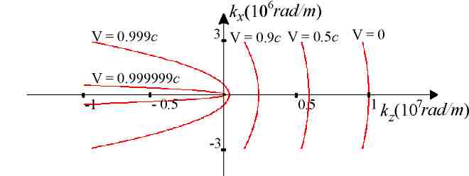
Figure 12: The support of angular spectrum of plane waves of a focused monochromatic beam as seen from inertial reference systems moving at different velocities relative to the rest system of the monochromatic beam ($k_{0}=1\times 10^{7}\frac{rad}{m}$). Due to the relativistiv Doppler shift the direction of propagation and the frequency of the monochromatic components of the focused beam transform so that the beam is seen as the FWM in the moving reference system.

Note that an alternate approach to describe the LW’s in terms of generalized Lorentz transforms can be found in Ref. lw6 – in this work it was shown that the superluminal and subluminal Lorentz transformations can be used to derive LW solutions to the scalar wave equation by boosting known solutions of the wave equation.

III.3.4 FWM’s as a construction of generalized functions in the Fourier domain

In Refs. fw15 ; fw16 Donnelly and Ziolkowski realized, that various separable and non-separable solutions to the wave equation can be constructed in spatial and temporal Fourier domain by choosing the Fourier transform of the solution of the differential equation so that, when multiplied by the transform of the particular differential operator, it gives zero in the sense of generalized functions. In the special case of scalar homogeneous wave equation the corresponding relation reads

$$\left(\chi^{2}+k_{z}^{2}-\frac{\omega^{2}}{c^{2}}\right)\psi\left(\mathbf{k},\omega\right)=0\text{,}$$ (110)

where $\psi\left(\mathbf{k},\omega\right)$ (9) is (3+1) dimensional Fourier transform of the solution of the wave equation (8). It can be shown that the function of the general type

$$\psi\left(\mathbf{k},\omega\right)=\Xi\left(\chi,\beta\right)\delta\left[k_{z}-\left(\beta-\frac{\chi^{2}}{4\beta}\right)\right]\delta\left[\omega-c\left(\beta+\frac{\chi^{2}}{4\beta}\right)\right]$$ (111)

satisfies (110) and yields all the known FWM’s (in the sense defined in this review). For example the choice fw15

$$\Xi\left(\chi,\beta\right)=\frac{\pi^{2}}{i\beta}\exp\left[-\frac{\chi^{2}a_{1}}{4\beta}\right]$$ (112)

leads to the original FWM’s.

One can notice, that if we eliminate the term $\chi^{2}/4\beta$ from the delta functions we get the condition (33) and thus the Eq. (111) is yet another transcription of the support of the angular spectrum of plane waves, derived in section III.1.1.

IV AN OUTLINE OF SCALAR LOCALIZED WAVES STUDIED IN LITERATURE SO FAR

IV.1 Introduction

Over the years a considerable effort has been made to find closed-form localized solutions to the homogeneous scalar wave equations. The main aim of this work is to study the feasibility of LW’s in optical domain. Without debasing the value of those solutions it appears, that this approach often leads to the source schemes that are difficult to realize even in radio frequency domain.

Though there has been several publications that provide an unified approach for the description of LW’s fw15 ; lw1 ; lw6 , to our best knowledge, the optical feasibility of those wave fields has not been estimated in literature. Moreover, the analysis of the numerical examples that have been published in literature show, that authors have often choose the parameters of the LW’s so that the frequency spectrum is in the radio frequency domain.

In our opinion in optical domain the best representation for the analysis is the Whittaker type plane wave decomposition. First of all, the mental picture of the Fourier lens that produces the two-dimensional Fourier transform of monochromatic wave field between its focal planes is often very useful in modeling the optical setups – we precisely know, how and in what approximations the elementary components of the Fourier picture, the plane waves and Bessel beams, can be generated. Secondly, the approach of the section III.1.5 allows us easily estimate the spatial shape of the wave fields under the discussion.

In the following overview we define the term ”optically feasible” by two rather obvious restrictions:

• The frequency spectrum of an optically feasible wave field should be in optical domain;

• The plane wave spectrum of an optically feasible wave field should not contain plane waves propagating at non-paraxial angles relative to optical axis.

The latter requirement can be justified by a very simple geometrical estimate, described in Fig. 29 – if the FWM’s has to propagate over distances that exceed the diameter of the source more than, say, five times, the maximum angle of the plane wave components in the wave field has to be less than $5$ degrees.

Note, that the energy content of most of the wave fields discussed in this outline is infinite, thus, they are not physically realizable as such. However, as we will see in chapters that follow, in optical implementations the finite energy approximations of the LW’s follow naturally from the finite aperture of the setups and this approximation do not change the general properties of the LW’s, so that the two conditions for optical feasibility, posed here, are also valid for LW’s with finite energy content.

In our numerical examples we try to optimize the parameters of each LW so that (i) the frequency spectrum of the wave fields extends from $\sim 0.5\times 10^{7}rad/m$ ($\sim 1100nm$ of wavelength) to $\sim 2\times 10^{7}rad/m$ ($\sim 300nm$ of wavelength), so that $\sigma_{k}\sim 3.8\times 10^{-7}m$ (65) for which the length of the corresponding plane wave pulse is $\sim 3fs$ – the shortest possible pulse length available, (ii) the plane wave with central wavelength propagate approximately at the angle $\approx 0.2{{}^{\circ}}$ relative to the propagation axis, giving $\sigma_{z}/\sigma_{\rho}\approx 0.003$ for the approximate ratio of pulse widths in $xy$ and $z$ direction. Note, that specifying the frequency range and cone angle of the Bessel beam of central wavelength completely determines the parameter $\beta$ – for $\gamma=1$ we have $\beta\approx 40rad/m$ (clarify section III.1.1).

IV.2 The original FWM’s

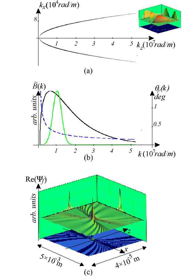
Figure 13: A numerical example of a FWM with the parameters $\gamma=1$, $\beta=40\frac{rad}{m}$, $a_{1}=1.4\times 10^{-7}m$: (a) The angular spectrum of plane waves in two perspectives; (b) The frequency spectrum of the FWM (black line), the frequency spectrum of an optically feasible wave field (green line), the angle $\theta_{F}\left(k\right)$ as the function of the wave number (dashed blue line); (c) The field distribution of the FWM.

With Eqs. (24a) and (24b) the angular spectrum of plane waves of the original scalar FWM’s in Eq. (29)

$$\Psi_{f}\left(\rho,z,t\right)=\exp\left[i\beta\mu\right]\frac{a_{1}}{4\pi i\left(a_{1}+i\zeta\right)}\exp\left[-\frac{\beta\rho^{2}}{a_{1}+i\zeta}\right]$$ (113)

can be derived from its bidirectional plane wave representation [fw14 ]

$$C_{0}\left(\tilde{\alpha},\tilde{\beta},\chi\right)=\frac{\pi}{2}\delta\left(\tilde{\beta}-2\beta\right)\exp\left[-\tilde{\alpha}a_{1}\right]\text{,}$$ (114)

giving

$$A_{0}\left(k,\theta\right)=\frac{\pi}{2}\exp\left[-\frac{a_{1}k\left(1+\cos\theta\right)}{2}\right]\delta\left(k-k\cos\theta-2\beta\right)$$ (115)

(see Fig. 13a). Inserting the angular spectrum (115) into integral representation of the type (17) yields

$$\Psi_{f}\left(\rho,z,t\right)=\int_{0}^{\infty}\mathrm{d}k~{}k\exp\left[-\frac{a_{1}k\left(1+\cos\theta_{F}\left(k\right)\right)}{2}\right]$$

$$\qquad\times J_{0}\left[k\rho\sin\theta_{F}\left(k\right)\right]\exp\left[ik\left(z\cos\theta_{F}\left(k\right)-ct\right)\right]$$ (116)

(as compared to (17) here we have taken into account the $1/k$ term that appears in (12) as to be consistent with [fw18 ] for example) so that the frequency spectrum of the superposition can be written as

$$\tilde{B}\left(k\right)=k\exp\left[-\frac{a_{1}k\left(1+\cos\theta_{F}\left(k\right)\right)}{2}\right]$$ (117)

[the significance of the factor $k\sin\theta_{F}\left(k\right)$ will be discussed in following sections].

The frequency spectrum $\tilde{B}\left(k\right)$ in Eq. (117) has two free parameters, $a_{1}$ and $\beta$, the latter having the same definition as in Eq. (30) of section III.1.1. As we already noted in the introduction of this chapter, the choice $\gamma=1$ together with the frequency range and cone angle of the Bessel beam of central wavelength determines $\beta=40rad/m$. The single free parameter is $a_{1}$ and a single parameter does not allow to approximate for any realistic light sources – Fig. 13b shows a typical spectrum that can be modeled in terms of Eq. (117) as compared to the optically feasible frequency spectrum specified in the introduction of this overview and it can be seen, that the bandwidth of the wave field is far beyond the reach of any realistic light source. In fact, due to this extraordinary large bandwidth the original FWM’s in Eq. (113) are essentially half-cycle pulses, as already noted in section III.3.2.

As deduced in section III.3.2 (and also in terms of the section III.1.5), the parameter $a_{1}$ determines the waist of the wave field – in our numerical example $a_{1}=1.4\times 10^{-7}$, so that the Eq. (100) gives

$$W_{0}=\sqrt{\frac{a_{1}}{\beta}}\sim 6\times 10^{-5}m\text{.}$$

In literature it has been argued, that the FWM’s determined by Eq. (113) are nonphysical as the wave field contain acausal components. In the discussion of Ref. fw18 it has been shown that the acausality can be eliminated by proper choice of parameters $a_{1}$ and $\beta$ – it has been shown that if $\beta a_{1}<1$, the predominant contribution to the spectrum comes from the plane waves moving in positive $z$ axis direction. In Fig 13b it can be seen, that this is indeed the case, however the field is still far from convenient for any optical implementation due to ultra-wide bandwidth.

Note, that various closed-form sub- and superluminal FWM’s ($\gamma\neq 1$) have been derived for example in Ref. fw15 .

IV.3 Bessel-Gauss pulses

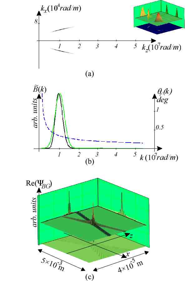
Figure 14: A numerical example of a Bessel-Gauss pulse optimized for optical generation with the parameters $\sigma=40000\frac{2\pi}{m}$, $a_{1}=5\times 10^{-6}m$, $\beta=40\frac{rad}{m}$, $\gamma=1$: (a) The angular spectrum of plane waves in two perspectives; (b) The frequency spectrum of the Bessel-Gauss pulse (black line), the frequency spectrum of an optically feasible wave field (green line), the angle $\theta_{F}\left(k\right)$ as the function of the wave number (dashed blue line); (c) The spatial field distribution of the pulse.

The Bessel-Gauss pulses were introduced by Overfelt in Ref. lw4 (see also Refs. fw15 ; g15 ; g25 ). In this publication it was shown, that the scalar wave field

$$\Psi_{BG}\left(\rho,\mu,\zeta\right) =\frac{a_{1}}{a_{1}+i\zeta}J_{0}\left(\frac{\kappa a_{1}\rho}{a_{1}+i\zeta}\right)\exp\left[i\beta\mu\right]$$

$$\times\exp\left[-\frac{\beta\rho^{2}}{a_{1}+i\zeta}\right]\exp\left[-i\frac{\kappa^{2}a_{1}\zeta}{4\beta\left[a_{1}+i\zeta\right]}\right]\text{,}$$ (118)

where the physical meaning of the parameters $a_{1}$, $\beta$, also $\zeta$ and $\mu$ is consistent with the previous discussion. The expression has an additional free parameter $\kappa$ as compared to the FWM’s in (113), in fact, the latter is the special case of the former in the limiting case $\kappa\rightarrow 0$. The Bessel-Gauss pulses were further investigated in Ref. fw15 where it was shown, that in Fourier picture as in Eq. (9) the spatiotemporal Fourier transform of the field can be written as

$$\psi_{BG}\left(\mathbf{k},\omega\right)=\Xi_{BG}\left(\chi,\beta\right)\delta\left[k_{z}-\left(\beta-\frac{\chi^{2}}{4\beta}\right)\right]\delta\left[\omega+c\left(\beta+\frac{\chi^{2}}{4\beta}\right)\right]\text{,}$$ (119)

where

$$\Xi_{BG}\left(\chi,\beta\right)=\frac{a_{1}4\pi^{3}}{\beta}I_{0}\left(\frac{\kappa a_{1}\chi}{2\beta}\right)\exp\left[-\frac{\kappa^{2}a_{1}}{4\beta}\right]\exp\left[-\frac{a_{1}\chi^{2}}{4\beta}\right]$$ (120)

(see section III.3.4 for the notation). From Eq. (119) it can be seen that the support of the plane wave spectrum of the Bessel-Gauss pulses is the same as described by Eq. (34) [or Eq. (37)]. The change of variables in (120) yields for the frequency spectrum

$$B\left(k\right) =\frac{a_{1}4\pi^{3}}{\beta}I_{0}\left(\frac{\kappa a_{1}k\sin\theta_{F}\left(k\right)}{2\beta}\right)$$

$$\times\exp\left[-\frac{a_{1}}{4\beta}\left(\kappa^{2}+k^{2}\sin^{2}\theta_{F}\left(k\right)\right)\right]\text{,}$$ (121)

where $\kappa>0$, $a_{1}>0$ and $\beta>0$.

In the original paper the Bessel-Gauss pulses were introduced as the wave fields that are ”more highly localized than the fundamental Gaussian solutions because of its extra spectral degree of freedom”. The additional free parameter is indeed advantageous, however, in our opinion not in the sense proposed in this publication – the spatial localization of any wideband free-space wave field is directly proportional to its bandwidth and the latter is inappropriately large even for the original FWM’s (see Ref. fw15 for a related discussion). It may be the consequence of this general emphasis of the original paper that it is not generally recognized that the extra parameter $\kappa$ in Eqs. (118) – (121) gives one the necessary degree of freedom to fit an arbitrary bandlimited Gaussian-like spectrum – from Eq. (121) it can be seen, that the central frequency and bandwidth of the spectra of the pulse are independently adjustable by the parameters $\kappa$ and $a_{1}$ respectively.

Analogously to the discussion in section III.3.2 the Bessel-Gauss pulses can be given the form that, in some respect, resembles that of the monochromatic Gaussian beam:

$$\Psi_{BG}\left(\rho,z,\zeta\right)=\exp\left[-i\beta\zeta\right]\frac{W_{0}}{a_{1}\left(\zeta\right)}J_{0}\left[\kappa a_{1}\rho\left(\frac{1}{\beta a_{1}^{2}\left(\zeta\right)}-i\frac{1}{R\left(\zeta\right)}\right)\right]$$

$$\qquad\times\exp\left[-\frac{\rho^{2}}{a_{1}^{2}\left(\zeta\right)}-\frac{\kappa^{2}a_{1}\zeta}{4\beta R\left(\zeta\right)}\right]$$ (122)

$$\times\exp\left[-i\left(\frac{\kappa^{2}a_{1}\zeta}{4\beta^{2}a_{1}^{2}\left(\zeta\right)}-\frac{\beta\rho^{2}}{R\left(\zeta\right)}\right)-i\left(\arctan\left(\frac{\zeta}{a_{1}}\right)-2\beta z+\frac{\pi}{2}\right)\right]\text{,}$$

here again

$$a_{1}\left(\zeta\right) =W_{0}\left[1+\left(\frac{\zeta}{a_{1}}\right)^{2}\right]^{\frac{1}{2}}$$ (123a)

$$R\left(\zeta\right) =\zeta\left[1+\left(\frac{a_{1}}{\zeta}\right)^{2}\right]$$ (123b)

$$W_{0} =\sqrt{\frac{a_{1}}{\beta}}\text{.}$$ (123c)

The general form of the Bessel-Gauss pulses (122) is very advantageous in the sense that here we can actually write out its carrier wave number – often this quantity is elusive for the wideband wave fields. Indeed, around the point $$\zeta=0 \rho=0 z$$, along the optical axis () with (123a) we can write for the axis component of the carrier wave number

$$k_{0z}=\beta+\frac{\sigma^{2}}{4\beta}-\frac{1}{a_{1}}$$ (124)

This result is actually quite significant, if we once more remind that in literature the FWM’s have often been termed as carrier-free wave fields (see Refs. g5 ; g10 for example). In lights of (124) we can conclude that the carrier-free behaviour of the FWM’s is indeed caused by the integral transform table, not by physical arguments.

In the numerical example in Fig. 14 we have optimized the parameters of the wave field as to match the spectral band specified in the introduction of this section. Again, the parameter $\beta$ is determined by the bandwidth and the cone angle of the central frequency as described above. Thus we got: $\sigma=40000\frac{rad}{m}$, $a_{1}=5\times 10^{-6}m$, $\beta=40\frac{rad}{m}$, $\gamma=1$. The evaluation of the Eq. (124) yields $k_{0z}=9.80004\times 10^{6}\frac{rad}{m}$ and this result is in good correspondence with the numerical simulations.

In conclusion, the Bessel-Gauss pulses are obviously much more appropriate for modeling realistic experimental situations.

IV.4 X-type wave fields

The X-type localized wave fields are characterized by that for their angular spectrum of plane waves $\beta=0$ in Eq. (34) [or $\xi=0$ in Eq. (37)]. This choice implies, that their support of angular spectrum of plane waves is a cone in $k$-space (see Fig. 2). Consequently, the phase and group velocity of X-type pulses are equal (both necessarily superluminal) and the field propagates without any local changes along the optical axis.

IV.4.1 Bessel beams

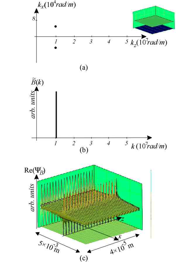
Figure 15: A numerical example of a monochromatic Bessel beam with the parameters $\theta_{0}=0.223\deg$, $k_{0}\sim 1\times 10^{7}$: (a) The angular spectrum of its plane waves in two perspectives; (b) The delta-shaped frequency spectrum; (c) The spatial field distribution of the beam.

The Bessel beams b1 –ba82 are the simplest special case of the propagation-invariant wave fields. Being the exact solutions to the Helmholtz equation in cylindrical coordinates their field reads as

$$\Psi_{B}\left(\rho,z,t\right)=\sum_{n}c_{n}~{}J_{n}\left(k\rho\sin\theta_{0}\right)\exp\left[in\phi\right]\exp\left[ik\left(z\cos\theta_{0}-ct\right)\right]$$ (125)

so that for the zeroth order Bessel beam we have

$$\Psi_{B}\left(\rho,z,t\right)=J_{0}\left(k\rho\sin\theta_{0}\right)\exp\left[ik\left(z\cos\theta_{0}-ct\right)\right]\text{.}$$ (126)

In the Fourier picture, the zeroth–order Bessel beam is the cylindrically symmetric superposition of the monochromatic plane waves propagating at angles $\theta_{0}$ relative to $z$ axis, correspondingly, their angular spectrum of plane waves in Eq. (18) reads

$$A_{0}^{\left(B\right)}\left(k,\theta\right)\sim~{}\delta\left(k-k_{0}\right)\delta\left(\theta-\theta_{0}\right)\text{.}$$ (127)

The bidirectional representation of the Bessel beam can be found in Ref. fw14 .

The properties of Bessel beams have been discussed in many publications both in terms of angular spectrum of plane waves b1 –b16 and diffraction theory ba5 –ba82 and their properties are very well understood today. The interest has been triggered in Refs. b1 ; b2 where Durnin et al presented them as ”nondiffracting” solutions of the homogeneous scalar wave equation – they demonstrated experimentally, that the central maximum of the Bessel beams propagates much further than the Rayleigh range predicts.

Note, that though there has been numerous experiments on Bessel beams, they are not realizable in experiment in the exact form (126) – indeed, the analysis of section III.2.3 immediately shows, that this wave field has both infinite total energy and energy flow over its cross-section. We will discuss this point in what follows.

In this review the Bessel beams appear as the components of the Fourier decomposition in Eqs. (15) – (17) for example. Later in this review we will refer to their most important properties in some detail. At this point we just depict its angular spectrum of plane waves with the typical field distribution (see Fig. 15).

IV.4.2 X-pulses

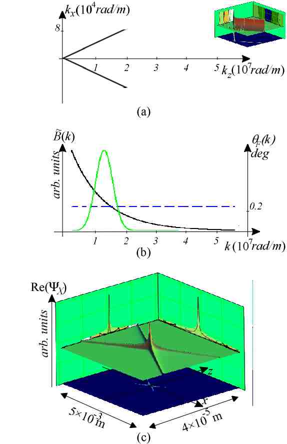
Figure 16: A numerical example of a X-pulse with the parameters $\theta_{0}=0.223\deg$, $\gamma=0.99999$: (a) The angular spectrum of plane waves in two perspectives; (b) The frequency spectrum of the X-pulse (black line), the frequency spectrum of an optically feasible wave field (green line), the angle $\theta_{0}$ as the (constant) function of the wave number (dashed blue line); (c) The spatial field distribution of the pulse.

In x1 Lu et al demonstrated that the choice

$$A_{0}^{\left(X\right)}\left(k,\theta\right)=B\left(k\right)\delta\left(\theta-\theta_{0}\right)$$ (128)

in representation (18) with the frequency spectrum

$$B\left(k\right)=\frac{1}{k^{2}}\exp\left[-ka_{0}\right]$$ (129)

yields the propagation-invariant wave field

$$\Psi_{X}\left(\rho,z,t\right)=\frac{a_{0}}{\sqrt{\left(\rho\sin\theta_{0}\right)^{2}+\left[a_{0}-i\left(z\cos\theta_{0}-ct\right)\right]^{2}}}$$ (130)

(see Ref. x4 for the description of higher order X-pulses). From the angular spectrum in Eq. (128) it can be seen, that the support of angular spectrum of plane waves of the X-pulses is a cone in $k$-space, i.e., all the plane wave components of the wave field propagate at the equal angle from the propagation axis. The frequency spectrum of X-pulses in Eq. (128) is uniform (see Fig. 16a) – the immediate conclusion of the approach of section III.1.5 that the corresponding field should have exponentially decaying behaviour in both $z$ axis and $xy$ plane is confirmed in Fig. 16c.

X-wave fields have been further investigated in Refs. x2 ; x3 ; x4 ; x5 , recently the topic have been given an overview and general description in Ref. x15 . We mention here the so called bowtie waves that are generally introduced as the derivatives of the X-waves:

$$\Psi_{mX}\left(\rho,z,t\right)=\frac{\partial^{m}\Psi^{\prime}\left(\mathbf{r},t\right)}{\partial x^{m}}\text{.}$$ (131)

The derivatives of X-waves have been shown to possess non-symmetric nature and have extended localization along a radial direction. In our terms the physical nature of such wave fields can be interpreted by applying the derivation operation on the general angular spectrum representation of the free-space scalar wave fields in Eq. (15). We easily get

$$\frac{\partial^{m}\Psi^{\prime}\left(\mathbf{r},t\right)}{\partial x^{m}}=\frac{1}{\left(2\pi\right)^{4}}\int_{0}^{\infty}\mathrm{d}k~{}k^{2}\int_{0}^{\pi}\mathrm{d}\theta\left(\sin\theta\right)^{m+1}\int_{0}^{2\pi}\mathrm{d}\phi\cos^{m}\phi$$

$$\qquad\times\mathbf{~{}}A\left(k\sin\theta\cos\phi,k\sin\theta\cos\phi,k\cos\theta\right)$$

$$\qquad\times\exp\left[ik\left(x\sin\theta\cos\phi+y\sin\theta\cos\phi+z\cos\theta-i\omega t\right)\right]\text{~{},}$$ (132)

so that the angular spectrum of plane waves of such wave fields is not cylindrically symmetric, correspondingly the wave field is a superposition of higher order monochromatic Bessel beams as described by Eq. (19) for example.

Due to the exponential shape of the frequency spectrum the X-waves are not appropriate for optical implementation.

IV.4.3 Bessel-X pulses

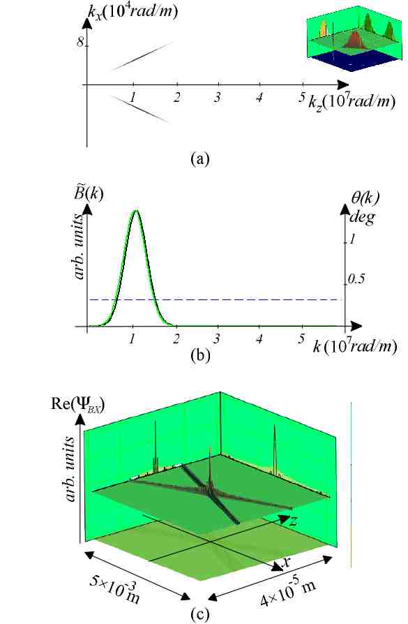
Figure 17: A numerical example of a Bessel-X pulse with the parameters $\theta_{0}=0.223\deg$, $\gamma=0.99999$: (a) The angular spectrum of plane waves in two perspectives; (b) The frequency spectrum of the Bessel-X pulse (black line) as compared to the frequency spectrum of an optically feasible wave field (green line), the angle $\theta_{0}$ as the (constant) function of the wavel number (dashed blue line); (c) The spatial field distribution of the pulse.

The Bessel-X pulses were introduced by Saari in Ref. bx0 ; bx1 as the bandlimited version of X-pulses. Their angular spectrum of plane waves can be described as

$$\tilde{A}_{0}^{\left(BX\right)}\left(k,\theta\right)=\tilde{B}\left(k\right)\delta\left(\theta-\theta_{0}\right)\text{,}$$ (133)

where

$$\tilde{B}\left(k\right)=\frac{\sigma_{k}}{\sqrt{2\pi}}\sqrt{\frac{k}{k_{0}}}\exp\left[-\frac{\sigma_{k}^{2}\left(k-k_{0}\right)^{2}}{2}\right]\text{,}$$ (134)

$\sigma_{k}$ being defined in (65) and $k_{0}$ being the carrier wave number, so that for the field one can write

$$\Psi_{BX}\left(\rho,z,t\right)=\int_{0}^{\infty}\mathrm{d}k~{}\tilde{B}\left(k\right)$$

$$\qquad\qquad\times J_{0}\left[k\rho\sin\theta_{0}\right]\exp\left[-ik\left(z\cos\theta_{0}-ct\right)\right]\text{.}$$ (135)

The integration in Eq. (18) can be carried out to yield bx1

$$\Psi_{BX}\left(\rho,z,t\right)=\sqrt{Z\left(d\right)}$$

$$\qquad\times\exp\left[-\frac{1}{2\sigma_{k}^{2}}\left(\rho^{2}\sin^{2}\theta+d^{2}\right)\right]J_{0}\left[Z\left(d\right)\rho k_{0}\sin\theta\right]\exp\left[ik_{0}d\right]\text{,}$$ (136)

where

$$Z\left(d\right)=1+\frac{id}{k_{0}\sigma_{k}^{2}}$$ (137)

and

$$d=z\cos\theta-ct\text{.}$$ (138)

From the Eqs. (133) and (134) it can be seen that,again, the support of angular spectrum of plane waves is a cone in $k$-space (see Fig. 17a). However, unlike the X-pulses, the frequency spectrum of Bessel-X pulse is Gaussian and it can be optimized to approximate that of our initial conditions. Thus, the Bessel-X pulses are optically feasible in the sense defined in this chapter.

IV.5 Two limiting cases of the propagation-invariance

IV.5.1 Pulsed wave fields with infinite group velocity

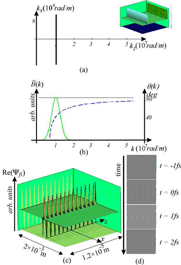
Figure 18: A numerical example of a the wave field with infinite group velocity with the parameters $\xi=6.7\times 10^{6}m$, $\gamma=\infty$: (a) The angular spectrum of plane waves in two perspectives; (b) The frequency spectrum of the pulse (black line), the frequency spectrum of an optically feasible wave field (green line), the angle $\theta_{F}\left(k\right)$ as the function of the wave number (dashed blue line), (c) The spatial field distribution of the pulse; (d) Three snapshots of the temporal evolution of the pulse.

Consider the special case $\gamma=0$ of the support of angular spectrum of plane waves (36) that reads

$$k_{z}\left(k\right)=\xi=const\text{.}$$ (139)

From the general definition of group velocity in Eq. (32) it is obvious, that for this particular case we have $v^{g}=\infty$. In what follows we give a physical description to the wave fields that have such a peculiar property.

A closed-form solution of the homogeneous scalar wave equation that obeys (139) can be easily found. The angular spectrum of plane waves of the wave field reads

$$A_{0}^{\left(fi\right)}\left(k,\theta\right)=B\left(k\right)\delta\left[\theta-\arccos\left(\frac{\xi}{k}\right)\right]\text{.}$$ (140)

The substitution in Whittaker type superposition (18) yields

$$\Psi_{fi}\left(\rho,z,t\right) =\int_{0}^{\infty}\mathrm{d}k\tilde{B}\left(k\right)J_{0}\left(k\rho\sqrt{1-\left(\frac{\xi}{k}\right)^{2}}\right)$$

$$\times\exp\left[ik\left(\frac{\xi}{k}z-ct\right)\right]\text{,}$$ (141)

where

$$\tilde{B}\left(k\right)=k^{2}\sqrt{1-\left(\frac{\xi}{k}\right)^{2}}B\left(k\right)\text{,}$$ (142)

so that

$$\Psi_{fi}\left(\rho,z,t\right)=\exp\left[i\xi z\right]\int_{0}^{\infty}\mathrm{d}k\tilde{B}\left(k\right)J_{0}\left(\rho\sqrt{k^{2}-\xi^{2}}\right)\exp\left[-ikct\right]\text{.}$$ (143)

If we choose $\tilde{B}\left(k\right)=const=1$ and use the integral transforms o9

$$\int_{0}^{\infty}\mathrm{d}xJ_{0}\left(b\sqrt{x^{2}-a^{2}}\right)\cos\left(xy\right)=\genfrac{\{}{.}{0.0pt}{1}{\left(b^{2}-y^{2}\right)^{-\frac{1}{2}}e^{-a\left(b^{2}-y^{2}\right)^{\frac{1}{2}}}\text{ \ \ \ \ \ \ \ if }0<y<b}{-\left(y^{2}-b^{2}\right)^{-\frac{1}{2}}\sin\left[a\left(y^{2}-b^{2}\right)^{\frac{1}{2}}\right]\text{ if }b<y<\infty}$$ (144)

and

$$\int_{0}^{\infty}\mathrm{d}xJ_{0}\left(b\sqrt{x^{2}-a^{2}}\right)\sin\left(xy\right)=\genfrac{\{}{.}{0.0pt}{1}{\;\;\;\;\;\;\;\;\;0\;\;\;\;\;\;\;\;\;\;\;\;\;\;\;\;\;\;\;\;\;\;\;\text{,if }\;\;\;\;0<y<b}{\left(y^{2}-b^{2}\right)^{-\frac{1}{2}}\cos\left[a\left(y^{2}-b^{2}\right)^{\frac{1}{2}}\right]\text{ if }b<y<\infty}$$ (145)

the integral (143) can be evaluated explicitly to yield

$$\Psi_{fi}\left(\rho,z,t\right)=\left\{\begin{array}[c]{c}\frac{\exp\left[i\xi z-i\xi\sqrt{\rho^{2}-c^{2}t^{2}}\right]}{\sqrt{\rho^{2}-c^{2}t^{2}}}\text{ if }0<tc<\rho\\ i\frac{\exp\left[i\xi z-\xi\sqrt{c^{2}t^{2}-\rho^{2}}\right]}{\sqrt{c^{2}t^{2}-\rho^{2}}}\text{ if }\rho<tc<\infty\end{array}\right.\text{.}$$ (146)

Note, that the special case $\xi=0$ yields the cylindrically symmetric superposition of plane wave pulses propagating perpendicularly to $z$ axis.

The support of the angular spectrum of plane waves of the wave field (146) is depicted in Fig. 18a. From the estimates of the spatial localization of LW’s in section III.1.5 we can expect the wave field to be localized in transversal direction at $t=0$, $z=0$ and to be uniform along the $z$ axis. Indeed, from the Fig. 18c it can be seen that at this space-time point the wave field (146) is an approximation to ”light filament” along the optical axis.

The temporal evolution of the wave field is depicted in Fig. 18d. One can see, that the effect of the infinite group velocity is that the light filament is focused only at a single time $t=0$ and extends from $-\infty$ to $\infty$. As to relate to the conventional wave optics, the temporal evolution of the light filament is a close relative to that of the plane wave pulse in a plane perpendicular to its wave vector.

As the wave field includes both non-optical frequencies and non-paraxial angles it is not optically feasible as such. However, it can be shown that a finite energy approximation to the light filament can in principle be generated by a cylindrical diffraction grating.

IV.5.2 Pulsed wave fields with frequency-independent beamwidth

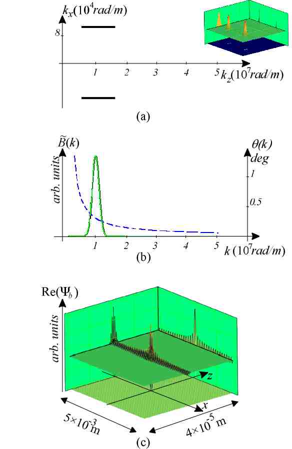
Figure 19: A numerical example of a the pulsed wave field with frequency independent beamwidth with the parameters $\alpha_{0}=4\times 10^{4}\frac{rad}{m}$, $\gamma\sim 0$: (a) The angular spectrum of plane waves in two perspectives; (b) The frequency spectrum of the pulse (black line), the frequency spectrum of an optically feasible wave field (green line), the cone angle of the component Bessel beams as the function of the wave number (dashed blue line); (c) The spatial field distribution of the pulse.

In Ref. lw7 Campbell et al introduced a wideband wave field that is a superposition of the Bessel beams the cone angle of which is chosen so that the condition

$$k\sin\theta\left(k\right)=\alpha_{0}=const$$ (147)

is satisfied for entire bandwidth. The condition (147) implies, that the transversal component of the wave vector of every plane wave component of the wave field is $\alpha_{0}$, the corresponding wave field was called as the pulsed wave fields with frequency independent beamwidth. The angular spectrum of plane waves for such choice can be written as

$$\tilde{A}_{0}^{\left(b\right)}\left(k,\theta\right)=\tilde{B}\left(k\right)\delta\left(\theta-\arcsin\left(\frac{\alpha_{0}}{k}\right)\right)\text{,}$$ (148)

so that the Whittaker superposition in Eq. (18) yields

$$\Psi_{b}\left(\rho,z,t\right)=J_{0}\left(\alpha_{0}\rho\right)\int_{0}^{\infty}\mathrm{d}k\tilde{B}\left(k\right)\exp\left[ik\left(z\sqrt{1-\left(\frac{\alpha_{0}}{k}\right)^{2}}-ct\right)\right]\text{,}$$ (149)

where

$$\tilde{B}\left(k\right)=\alpha_{0}k^{2}~{}B\left(k\right)\text{.}$$ (150)

The support of the angular spectrum of plane waves of the wave field Eq. (149) is depicted in Fig. 19 (in the numerical example the frequency spectrum $B\left(k\right)$ is Gaussian with the bandwidth corresponding to $\sim 6fs$ pulse). Using the approach of section III.1.5 one can immediately tell the general spatial shape of such wave fields. Indeed, in this case we have a simple special case, where the projection of the angular spectrum of plane waves onto the $k_{x}k_{y}$-plane is delta-ring, correspondingly, the field in transversal direction at $z=0$, $t=0$ should be of the shape of the Bessel function. As for longitudinal shape, its envelope is determined by the bandwidth by it Fourier transform, i.e., we should have a slice of a Bessel beam. The numerical simulation in Fig. 19d shows that this estimate is true. Also, one can see that the wave field has generally infinite energy flow.

Comparing the support in Eq. (148) to that of the propagation-invariant pulsed wave field in Eq. (34) and (40) one can see, that the wave field (149) is not propagation-invariant. Consequently, the localized part of the wave field spreads as it propagates. We can also suggest the best condition for limited propagation-invariance – the comparison of the support in Fig. 19a to those of FWM’s in Fig. 2 implies that for restricted bandwidths the support (147) could be optimized to approximate the ”horizontal” part of the ellipsoidal supports of the subluminal FWM’s ($\gamma>1$).

IV.6 Physically realizable approximations to FWM’s

As it was explained in section III.1.5, the presence of the delta function in the support of the angular spectrum of plane waves of the free-space scalar wave fields necessarily results in infinite total energy content of the wave field. Consequently, for all the above reviewed wave fields the total energy content is infinite,

$$U_{tot}=\int_{-\infty}^{\infty}\mathrm{d}z\int_{0}^{\infty}\mathrm{d}\rho\rho\int_{0}^{2\pi}\mathrm{d}\varphi\left|\Psi_{F}\left(\rho,z,\varphi,t\right)\right|^{2}=\infty\text{.}$$ (151)

Here we proceed by reviewing the approaches used in literature to overcome this difficulty. In later chapters we introduce the approach that is especially useful for analyzing optical experiments.

IV.6.1 Electromagnetic directed-energy pulse trains (EDEPT)

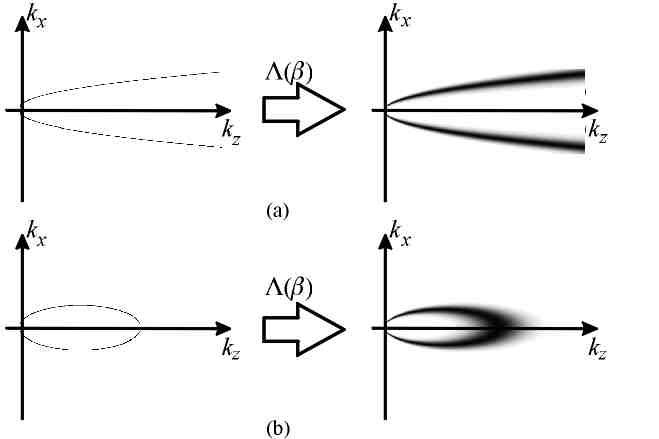
Figure 20: On the effect of integrating over the parameter $\beta$ on the support of the angular spectrum of plane waves of the FWM’s: (a) The special case of the ”mean” support of the angular spectrum of plane waves where $\gamma=1$ ($v^{g}=c$), $\beta\neq 0$; (b) The special case where $\gamma>0$ ($v^{g}<c$), again, $\beta\neq 0$.

One approach has been to construct various continuous superpositions of FWM’s (113) over the parameter $\beta$ (see Refs. fw5 ; fw14 ; fw15 ; lw1 and references therein), in this case one writes

$$\Psi_{LW}\left(z,\rho,t\right) =\int_{0}^{\infty}\mathrm{d}\beta\Lambda\left(\beta\right)\Psi_{F}\left(z,\rho,t;\beta\right)$$

$$=\frac{a_{1}}{4\pi i\left(a_{1}+i\zeta\right)}\int_{0}^{\infty}\mathrm{d}\beta\Lambda\left(\beta\right)\exp\left[s\left(z,\rho,t\right)\right]\text{,}$$ (152)

where

$$s\left(z,\rho,t\right)=-\frac{\beta\rho^{2}}{a_{1}+i\zeta}+i\beta\left(z+ct\right)$$ (153)

$\Lambda\left(\beta\right)$ is a weighting function and the subscript $LW$ means ”localized wave”. As the supports of the angular spectrum of the FWM’s for different values of parameter $\beta$ generally do not overlap and change smoothly in $k$-space, the integration indeed eliminates the delta function in the expression for angular spectrum of plane waves (see Fig. 20). It can be shown lw1 that Eq. (152) yields finite total energy wave field if only the function $\Lambda\left(\beta\right)$ satisfies condition

$$\frac{1}{2a_{1}}\int_{0}^{\infty}\mathrm{d}\beta\left|\Lambda\left(\beta\right)\right|^{2}\frac{1}{\beta}<\infty$$ (154)

(see Eq. 2.8 of Ref. lw1 ), i.e., if only $\beta^{-1/2}\Lambda\left(\beta\right)$ is square integrable. The LW’s of the general form (152) have been called EDEPT solutions of the scalar wave equation.

From the discussion of previous chapters it is obvious, that the wave field of the general form (152) are not strictly propagation-invariant. At first glance it may seem surprising because (i) FWM solutions with different values of parameter $\beta$ do travel without any spread and (ii) all the FWM’s overlap in every space-time point as their group velocities are equal. However, the effect can be easily understood if we recollect from section III.3.1 that the phase velocities of the pulses are different leading to the $z$ axis position dependent interference and spread of the superposition of the component pulses (see Ref. fw3 ; fw3o1 for alternate proofs of this claim).

Modified power spectrum pulse (MPS)

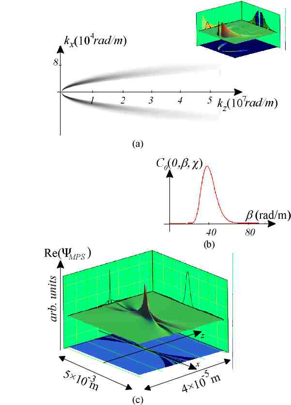
Figure 21: A numerical example of a MPS with the parameters $a_{1}=1.4\times 10^{-7}m$, $a_{2}=4000m$, $q=10$, $p=0.0001$, $b=0.002$, ($\gamma=1$, $\beta_{0}=40\frac{rad}{m}$): (a) The angular spectrum of plane waves in two perspectives; (b) The $\beta$ -distribution in bidirectional plane wave spectrum for $\alpha=0$; (c) The spatial field distribution of the MPS for $t=0$.

The modified power spectrum pulses lw1 have been introduced by the following bidirectional plane wave spectrum (see Eq. (3.3) of Ref. lw1 and Eq. (3.32) of Ref. fw14 )

$$C_{0}^{\left(m\right)}\left(\tilde{\alpha},\tilde{\beta},\chi\right)=\left\{\begin{array}[c]{c}\frac{p\left(p\tilde{\beta}-b\right)^{q-1}}{2\pi\Gamma\left(q\right)}\exp\left[-\left(\tilde{\alpha}a_{1}+\left(p\tilde{\beta}-b\right)a_{2}\right)\right],\,\text{if}\,\tilde{\beta}>\frac{b}{p}\\ 0\quad\quad\quad\quad\quad\quad\quad\quad\quad\quad\quad\text{, if }\frac{b}{p}>\tilde{\beta}\geq 0\end{array}\right.\text{.}$$ (155)

Here $a_{2}$, $b$, $q$ and $p$ are new parameters and $\Gamma$ denotes the gamma function. Using the relations (24a) and (24b) the corresponding Whittaker type plane wave spectrum can be written as (see also Eq. (3.13a) and (3.13b) of Ref. lw1 )

$$\tilde{A}_{0}^{\left(MPS\right)}\left(\chi,k_{z}\right)=\left\{\genfrac{}{}{0.0pt}{0}{\begin{array}[c]{c}\frac{p\left[\frac{p}{2}\left(k-k_{z}\right)-b\right]^{q-1}}{2\pi\Gamma\left(q\right)}\exp\left[-\frac{\left(k+k_{z}\right)a_{1}}{2}+\left(b-\frac{\left(k-k_{z}\right)p}{2}\right)a_{2}\right]\\ \quad\quad\quad\quad\quad\quad\quad\quad\text{,~{}if}\,k_{z}<\frac{p}{b}\frac{\chi^{2}}{4}-\frac{b}{p}\end{array}}{\begin{array}[c]{c}\\ \quad 0\quad\quad\quad\quad\quad\quad\text{, if }k_{z}>\frac{p}{b}\frac{\chi^{2}}{4}-\frac{b}{p}\end{array}}\right.\text{,}$$ (156)

where $k=\sqrt{\chi^{2}+k_{z}^{2}}$ and the relation (26) has been used. The field function of the MPS’s is described by equation (see Eqs. (3.34) and (1.4) of Ref. fw14 )

$$\Psi_{MPS}\left(\rho,\zeta,\eta\right)=\left[\frac{1}{4\pi\left(a_{1}+i\zeta\right)}\frac{\exp\left(-\frac{bs}{p}\right)}{\left(a_{2}+\frac{s}{p}\right)^{q}}\right]\text{,}$$ (157)

where

$$s=\frac{\rho^{2}}{4\pi\left(a_{1}+i\zeta\right)}-i\eta\text{.}$$ (158)

The comparison of the bidirectional plane wave spectra of MPS (155) with that of the FWM’s (114) one can see, that the latter is a special case $a_{2}=0$, $q=1$ of the former. Consequently, the parameter $a_{1}$ in (155) has the same interpretation as in case of FWM’s – it determines the frequency spectra of the wave field. From (156) it is also obvious that the parameter $a_{2}$ determines the width of the $\beta$ distribution and parameter $b$ determines the central value of $\beta$. As for parameter $q$, it can be used to optimize the shape of the $\beta$ distribution.

A numerical example of the MPS is depicted in Fig. 21. In this example we tried to optimize the parameters so as to satisfy the conditions for optical feasibility as stated in the introduction of this overview. From the angular spectrum of plane waves in Fig. 21a one can see, that the MPS’s generally have the same inconvenience as FWM’s – there no freedom to choose the frequency spectrum as to optimize for any convenient light source and they are generally half-cycle pulses.

For an interpretation of MPS’s as being the field generated by a combined point-like source and a sink placed at a complex-number coordinate see Refs. go35 ; go40

It is not our aim at this point to study the temporal behaviour of the EDEPT solutions, thus, the wave field is calculated only for the time $t=0$.

IV.6.2 Splash pulses

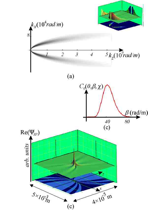
Figure 22: A numerical example of a Splash mode with the parameters $a_{1}=1.4\times 10^{-7}m$, $a_{2}=0.4m$, $q=16$, ($\gamma=1$, $\beta_{0}=40\frac{rad}{m}$): (a) The angular spectrum of plane waves in two perspectives; (b) The $\beta$ -distribution in bidirectional plane wave spectrum for $\tilde{\alpha}=0$; (c) The spatial field distribution of the Splash mode for $t=0$.

Splash pulses fw5 appear if one chooses the bidirectional plane wave spectrum as (Eq. (3.13) of Ref. fw14 )

$$C_{0}^{\left(SP\right)}\left(\tilde{\alpha},\tilde{\beta},\chi\right)=\frac{\pi}{2}\tilde{\beta}^{q-1}\exp\left[-\left(\tilde{\alpha}a_{1}+\tilde{\beta}a_{2}\right)\right]\text{.}$$ (159)

One can see, that the bidirectional spectrum is similar in the structure as the one of the MPS (155). Here again the term $\exp\left[-\tilde{\alpha}a_{1}\right]$ can be interpreted as the spectra of the ”central” FWM and the parameters $a_{2}$ and $q$ determine the distribution function over the parameter $\tilde{\beta}$. The integration in the bidirectional plane wave decomposition (22) can be carried out to yield (Eq. (3.19) of Ref. fw14 , Eq. (17) of Ref. fw5 )

$$\Psi_{SP}\left(\rho,\zeta,\eta\right)=\frac{\Gamma\left(q\right)}{4\pi\left(a_{1}+i\zeta\right)}\left[\left(a_{2}-i\eta\right)+\frac{1}{\left(a_{1}+i\zeta\right)}\right]$$ (160)

The wave field has been called as ”splash pulse” in Ref. fw5 as for its characteristic spatial shape. However, in our numerical example we tried once more to find a set of parameters suitable for optical generation. It appeared (see Fig. 22), that in this case the angular spectrum of plane waves is very similar to that of the MPS’s as in Fig. 21.

IV.7 Several more LW’s

To date, the literature on LW’s and on propagation of ultrashort electromagnetic pulses is overwhelming and this overview is by no means complete. Our aim was to demonstrate the applicability of our approach on most important special cases.

As already mentioned, in Ref. lw6 Besieris et al derived several closed-form superluminal and subluminal LW solutions to the scalar wave equation by ”boosting” known solutions of other Lorentz invariant equations.

In section III.3.4, we already reviewed the approach of solving the homogeneous scalar wave equation and Klein-Gordon equation, introduced in Refs. fw15 ; fw16 by Donnelly and Ziolkowski. In those works, they also deduced various closed-form separable and non-separable solutions to the wave equation.

In Ref. lw3 Overfelt found a continua of localized wave solutions to the scalar homogeneous wave, damped wave, and Klein-Gordon equations by means of a complex similarity transform technic.

The numerous publications that are involved with ultrashort-pulse solutions of the time-dependent paraxial wave equation (e.g. isodiffracting pulses) should be mentioned here (see Refs. go15 –go40 and references therein).

IV.8 On the transition to the vector theory

Even though the scalar theory is often used in description of propagation of electromagnetic wave fields, generally the solutions to the Maxwell equations have to be used. However, the latter approach is generally much more involved.

In the context of this review, we investigate the free-space wave fields and mostly use the angular spectrum representation of the wave fields. In this context the limitations of the scalar theory can be easily formulated – the scalar theory is reasonably accurate if only the plane wave components of the wave field propagate at small (paraxial) angles relative to optical axis (see Wolf and Mandel ok4 , for example). In this review we investigate the possibilities of optical generation of FWM’s (and LW’s), correspondingly, the above formulated restriction is satisfied in all practical cases and we can restrict ourselves to scalar theory.

(Of course, this is not the case with the original FWM’s and LW’s published in literature – the plane wave components of those wave fields propagate even perpendicularly to the direction of propagation and in their exact description the transition to the vector theory is obligatory.)

The vector theory of FWM’s and LW’s has been formulated and used in several publications fw1 ; fw2 ; fw3 ; fw8 ; lw1 ; ve20 ; ve30 ; ve35 ; x7 . The preferred approach has been the use of the Hertz vectors as formulated in Eqs. (7a) and (7b). One can refer to the theory expounded by Ziolkowski lw1 where he used the Hertz vectors of the form

$$\mathbf{\Pi}^{\left(e\right)} =\mathbf{z~{}}\Psi_{F}$$ (161a)

$$\mathbf{\Pi}^{\left(m\right)} =\mathbf{z~{}}\Psi_{F}\text{,}$$ (161b)

where $$\mathbf{z} \Psi_{F} \mathbf{z} \Psi_{i}$$ is the unit vector along the propagation axis and is the (localized) solution of the scalar wave equation. With (161a) and (161b) one get TE or TM field with respect to respectively. A more general treatment can be found in Ref. ve35 , where the Hertz vectors are written as the superpositions of the solutions of scalar wave equation as

$$\mathbf{\Pi}^{\left(m\right)} =\mathbf{x}\sum_{p}a_{p}^{\left(m\right)}\Psi_{p}+\mathbf{y}\sum_{q}b_{q}^{\left(m\right)}\Psi_{q}+\mathbf{z}\sum_{s}c_{s}^{\left(m\right)}\Psi_{s}$$ (162a)

$$\mathbf{\Pi}^{\left(e\right)} =\mathbf{x}\sum_{p}a_{p}^{\left(e\right)}\Psi_{p}+\mathbf{y}\sum_{q}b_{q}^{\left(e\right)}\Psi_{q}+\mathbf{z}\sum_{s}c_{s}^{\left(e\right)}\Psi_{s}\text{.}$$ (162b)

The computation of the field components using (7a) and (7b), although straightforward, results in very complex formulas.

The intuitive analysis of the effect of the transfer to exact vector theory that is more in the spirit of this review can be carried out in terms of the results that have been published on vector Bessel beams in Refs. ve10 ; ve12 ; ve25 ; si10 . For example, the result in Ref. si10 reveals, that for TE and TM fields the vector Bessel beams retain their paraxial-Bessel beam nature up to cone angles $\sim 14{{}^{\circ}}$ and this result indeed amply justifies the use of the scalar theory in this review.

IV.8.1 The derivation of vector FWM’s by directly applying the Maxwell’s equations

To finish this chapter we nevertheless advance in some extent the second approach mentioned in Sec. II.1, where we gave the general expression for the plane wave decomposition of the solution of the free-space Maxwell equations.

To find the vector form for the FWM’s as described in Eq. (42) we use the Eqs. (3a) – (5c). In correspondence with Eq. (35) we choose

$$\mathcal{E}_{x}\left(\mathbf{k},\omega\right) =\mathcal{\tilde{E}}_{x}\left(k,\phi\right)\delta\left[k_{z}-k\cos\theta_{F}\left(k\right)\right]$$ (163)

$$\mathcal{E}_{y}\left(\mathbf{k},\omega\right) =\mathcal{\tilde{E}}_{y}\left(k,\phi\right)\delta\left[k_{z}-k\cos\theta_{F}\left(k\right)\right]$$ (164)

and this choice yields from Eq. (3a) and (3b)

$$E_{i}\left(\mathbf{r},t\right) =\frac{1}{\left(2\pi\right)^{4}}\exp\left[-2i\beta\gamma z\right]$$ (165)

$$\times\int_{0}^{2\pi}\mathrm{d}\phi\int_{-\infty}^{\infty}\mathrm{d}kk^{2}\sin\theta_{F}\left(k\right)~{}\mathcal{\tilde{E}}_{i}\left(k,\phi\right)\times$$

$$\times\exp\left[ik\left(x\sin\theta_{F}\left(k\right)\cos\phi+y\sin\theta_{F}\left(k\right)\sin\phi+\gamma z-ct\right)\right]\text{,}$$

$$H_{i}\left(\mathbf{r},t\right) =\frac{1}{\left(2\pi\right)^{4}}\exp\left[-2i\beta\gamma z\right]$$ (166)

$$\times\int_{0}^{2\pi}\mathrm{d}\phi\int_{-\infty}^{\infty}\mathrm{d}kk^{2}\sin\theta_{F}\left(k\right)\mathbf{~{}}\mathcal{\tilde{H}}_{i}\left(k,\phi\right)$$

$$\times\exp\left[ik\left(x\sin\theta_{F}\left(k\right)\cos\phi+y\sin\theta_{F}\left(k\right)\sin\phi+\gamma z-ct\right)\right]\text{,}$$

where from Eqs. (4) – (5c)

$$\mathcal{\tilde{E}}_{z}\left(k,\phi\right)=-\tan\theta_{F}\left(k\right)\left[\cos\phi\mathcal{\tilde{E}}_{x}\left(k,\phi\right)+\sin\phi\mathcal{\tilde{E}}_{y}\left(k,\phi\right)\right]$$ (167)

and

$$\mathcal{\tilde{H}}_{x}\left(k,\phi\right) =-\frac{1}{c\mu_{0}\cos\theta_{F}\left(k\right)}\left[\sin^{2}\theta_{F}\left(k\right)\sin\phi\cos\phi\mathcal{\tilde{E}}_{x}\left(k,\phi\right)+\right.$$

$$\left.+\left(1-\sin^{2}\theta_{F}\left(k\right)\cos^{2}\phi\right)\mathcal{\tilde{E}}_{y}\left(\phi,k\right)\right]$$ (168)

$$\mathcal{\tilde{H}}_{y}\left(k,\phi\right) =\frac{k}{c\mu_{0}\cos\theta_{F}\left(k\right)}\left[\left(1-\sin^{2}\theta_{F}\left(k\right)\sin^{2}\phi\right)\mathcal{\tilde{E}}_{x}\left(k,\phi\right)+\right.$$

$$\left.+\sin^{2}\theta_{F}\left(k\right)\sin\phi\cos\phi\mathcal{\tilde{E}}_{y}\left(k,\phi\right)\right]$$ (169)

$$\mathcal{\tilde{H}}_{z}\left(k,\phi\right)=\frac{1}{c\mu_{0}}\sin\theta_{F}\left(k\right)\left[\sin\phi\mathcal{\tilde{E}}_{x}\left(k,\phi\right)-\cos\phi\mathcal{\tilde{E}}_{y}\left(k,\phi\right)\right]\text{.}$$ (170)

By expanding

$$\mathcal{\tilde{E}}_{i}\left(k,\phi\right)=\sum_{n=-\infty}^{\infty}\mathcal{\tilde{E}}_{i}\left(k,n\right)\exp\left[in\phi\right]\text{,}$$ (171)

where

$$\mathcal{\tilde{E}}_{i}\left(k,n\right)=\frac{1}{2\pi}\int_{0}^{2\pi}d\phi\mathcal{\tilde{E}}_{i}\left(k,\phi\right)\exp\left[-in\phi\right]\text{,}$$ (172)

the integration over the $\phi$ can be carried out to yield

$$E_{i}\left(\mathbf{r},t\right) =\frac{1}{\left(2\pi\right)^{2}}\exp\left[-2i\beta\gamma z\right]\sum_{n}\int_{-\infty}^{\infty}\mathrm{d}k$$

$$\times\exp\left[in\phi\right]L_{i}^{\mathcal{E}}\left(k,\rho,n\right)\exp\left[ik\left(\gamma z-ct\right)\right]$$ (173)

$$H_{i}\left(\mathbf{r},t\right) =\frac{1}{\left(2\pi\right)^{2}}\exp\left[-2i\beta\gamma z\right]\sum_{n}\int_{-\infty}^{\infty}\mathrm{d}k$$

$$\times\exp\left[in\phi\right]L_{i}^{\mathcal{H}}\left(k,\rho,n\right)\exp\left[ik\left(\gamma z-ct\right)\right]\text{,}$$ (174)

where

$$L_{x}^{\mathcal{E}}\left(k,\rho,n\right)=k^{2}\sin\theta_{F}\left(k\right)~{}\mathcal{\tilde{E}}_{x}\left(k,n\right)J_{n}\left(k\rho\sin\theta_{F}\left(k\right)\right)$$ (175)

$$L_{y}^{\mathcal{E}}\left(k,\rho,n\right)=k^{2}\sin\theta_{F}\left(k\right)~{}\mathcal{\tilde{E}}_{y}\left(k,n\right)J_{n}\left(k\rho\sin\theta_{F}\left(k\right)\right)$$ (176)

and $L_{z}^{\mathcal{E}}\left(k,n,\rho\right)$, $L_{i}^{\mathcal{H}}\left(k,\rho,n\right)$ can be expressed as the linear combinations of Bessel functions of different order. (see Refs. ve12 ; si10 ; si30 for relevant discussions).

We also note, that in addition to the TM and TE wave fields azimuthally polarized, radially polarized and circularly polarized vector FWM’s can be derived si10 .

IV.9 Conclusions.

The main conclusion of this section are:

• At this point it should be clear, that all the possible closed-form FWM’s can be analyzed in a single framework where the support of the angular spectrum of plane waves (34) – (40) is the only definitive property for propagation-invariance. The question of whether an integration over the support has or has not a closed-form result is the question of mathematical convenience only.

• With a proper choice of parameters some of the closed form FWM’s (Bessel-Gauss pulses, Bessel-X) are well suited for use as the models for simulating the result of optical experiments. In contrary, the LW’s we reviewed here – the MPS’s, splash pulses and the original FWM’s – are not feasible in this context. Mostly it is because of the ultra-wide bandwidth and non-paraxial angular spectrum content of the pulses.

• In our opinion, the procedure of modeling finite-thickness supports for finite energy approximations of FWM’s reviewed in this section lacks a convenient physical interpretation and to estimate its practical value this topic has to be addressed in the context of a particular launching setup instead.

V LOCALIZED WAVES IN THE THEORY OF PARTIALLY COHERENT WAVE FIELDS

Every electromagnetic field in nature has some fluctuations associated with it– even the purest laser light is not exactly coherent. However, in optical region the fluctuations are too rapid for direct measurement. Their existence can be deduced from suitable experiments where the correlation between these fluctuations of field variables at two or more space-time points are measured. The second-order coherence theory gives a precise measure of those correlations for any two space-time points and formulates the dynamic laws which the corresponding correlation functions obey. It provides a unified treatment of all well-known interference and polarization phenomena of traditional optics.

Our interest in introduction of the coherence theory is two-fold. First of all, we can generalize the concept of propagation-invariance into the more general class of optical fields where the (idealistic) fully coherent laser light is but a special case. As the consequence we not only obtain a more general view of the subject but also a practical approach towards the experimental evidence of validity of the theory presented above.

In what follows we again confine ourselves to free fields only, i.e., within the spatiotemporal domain the fields under investigation do not contain sources (except perhaps at infinity) and they do not interact with any material objects.

V.1 Propagation-invariance in domain of partially coherent fields in second order coherence theory

V.1.1 General definitions

Let us start with some general notion on the subject (see Ref. ok4 ). The definitive characteristics of a (generally) stochastic wave field in second order coherence theory is the ensemble cross-correlation function, often named as mutual coherence function for two points that can be defined as

$$\Gamma\left(\mathbf{r}_{1},\mathbf{r}_{2},t_{1},t_{2}\right)=\left\langle V^{\ast}(\mathbf{r}_{1},t_{1})V(\mathbf{r}_{2},t_{2})\right\rangle_{e}\text{.}$$ (177)

In this equation $V(\mathbf{r},t)$ is the (complex) field of a particular realization of a source-free scalar field and angle brackets denote the averaging over the ensemble of realizations, in essence the function ”measure” the correlation that exists between the light vibrations of field $V\left(\mathbf{r},t\right)$ at the space-time points $\left(\mathbf{r}_{1},t_{1}\right)$ and $\left(\mathbf{r}_{2},t_{2}\right)$ (in terms of statistics the two could be called processes). The direct calculation of ensemble averages for such two stochastic processes generally requires determination of their joint (two-fold) probability densities $p_{2}$, with which one can write

$$\Gamma\left(\mathbf{r}_{1},\mathbf{r}_{2},t_{1},t_{2}\right)=\int\int V_{1}^{\ast}V_{2}p_{2}\left[V_{1}^{\ast},\mathbf{r}_{1},t_{1};V_{2}\mathbf{r}_{2},t_{2}\right]\mathrm{d}V_{1}^{\ast}\mathrm{d}V_{2}\text{,}$$ (178)

where we have denoted the continuous set of field values in the two space-time points as

$$V_{i}=V(\mathbf{r}_{i},t_{i})\text{, \quad}\,i=1,2\text{.}$$ (179)

The joint probability density is generally unknown, however, there are several special cases for which the mutual coherence function can be directly calculated. For example, the two processes, $V_{1}$ and $V_{2}$ can be statistically independent of each other, in this case the joint probability density is completely separable:

$$p_{2}\left[V_{1}^{\ast},\mathbf{r}_{1},t_{1};V_{2}\mathbf{r}_{2},t_{2}\right]=p_{1}\left(V_{1}^{\ast},\mathbf{r}_{1},t_{1}\right)p_{1}\left(V_{2},\mathbf{r}_{2},t_{2}\right)\text{,}$$ (180)

so that the mutual coherence function is also separable, giving

$$\Gamma\left(\mathbf{r}_{1},\mathbf{r}_{2},t_{1},t_{2}\right) =\int V_{1}^{\ast}p_{1}\left(V_{1}^{\ast},\mathbf{r}_{1},t_{1}\right)\mathrm{d}V_{1}^{\ast}\int V_{2}p_{1}\left(V_{2},\mathbf{r}_{2},t_{2}\right)\mathrm{d}V_{2}$$

$$=\left\langle V^{\ast}(\mathbf{r}_{1},t_{1})\right\rangle_{e}\left\langle V(\mathbf{r}_{2},t_{2})\right\rangle_{e}\text{,}$$ (181)

where $p_{1}$ is the first order probability density. The second well-known limiting case is the complete correlation (or complete mutual coherence) between the two processes. In this case the knowledge of one process completely determines the second process, so that the two processes as well as the field $V(\mathbf{r},t)$ are non-stochastic in nature. The first order probability density then have to have the form

$$p_{1}\left(V,\mathbf{r,}t\right)=\delta\left(V-V_{c}\left(\mathbf{r,}t\right)\right)\text{,}$$ (182)

where $V_{c}\left(\mathbf{r,}t\right)$ is the deterministic function of the space-time point. For the second order probability density we have

$$p_{2}\left[V_{1}^{\ast},\mathbf{r}_{1},t_{1};V_{2},\mathbf{r}_{2},t_{2}\right]=\delta\left(V_{1}^{\ast}-V_{c}^{\ast}\left(\mathbf{r}_{1}\mathbf{,}t_{1}\right)\right)\delta\left(V_{2}-V_{c}\left(\mathbf{r}_{2}\mathbf{,}t_{2}\right)\right)$$ (183)

and for the mutual coherence function of the coherent wave field

$$\Gamma\left(\mathbf{r}_{1},\mathbf{r}_{2},t_{1},t_{2}\right)=V_{c}^{\ast}\left(\mathbf{r}_{1}\mathbf{,}t_{1}\right)V_{c}\left(\mathbf{r}_{2}\mathbf{,}t_{2}\right)\text{.}$$ (184)

The third special case is the stationary stochastic field. The random process is said to be stationary if all the probability densities governing the fluctuations of the field are invariant under an arbitrary translation of the origin of time, i.e., if

$$p_{1}\left[V_{1}^{\ast},\mathbf{r}_{1},t\right] =p_{1}\left[V_{1}^{\ast},\mathbf{r}_{1},t_{1}+T\right]$$ (185)

$$p_{2}\left[V_{1}^{\ast},\mathbf{r}_{1},t_{1};V_{2},\mathbf{r}_{2},t_{2}\right] =p_{2}\left[V_{1}^{\ast},\mathbf{r}_{1},t_{1}+T;V_{2},\mathbf{r}_{2},t_{2}+T\right]\text{.}$$ (186)

In this case the mutual coherence function depends only on the difference of time, so that it is often written as

$$\Gamma\left(\mathbf{r}_{1},\mathbf{r}_{2},t_{2},t_{1}\right)=\Gamma\left(\mathbf{r}_{1},\mathbf{r}_{2},t_{2}-t_{1}\right)\text{.}$$ (187)

Note, that for the statistically independent processes the conditions (180) and (185) imply that $\Gamma\left(\mathbf{r}_{1},\mathbf{r}_{2},t_{1},t_{2}\right)\equiv 0$.

The above definitions are of general nature. Let us now constraint ourselves to the stochastic superpositions of solutions of scalar wave fields. In our context we could proceed as follows. For scalar wave fields the general stochastic process $V(\mathbf{r},t)$ should satisfy the homogeneous scalar wave equation and this obviously implies certain restrictions to the form of the corresponding mutual coherence function. In the context of present study the most convenient way to introduce them is to represent the field as the Whittaker-type plane wave expansion:

$$V(\mathbf{r},t)=\int_{0}^{\infty}dk\int_{0}^{\pi}d\theta\int_{0}^{2\pi}d\phi\ a(k,\theta,\phi)\ \exp\left[ik\left(\mathbf{rn}-ct\right)\right]\text{,}$$ (188)

where $a(k,\theta,\phi)$ is the stochastic, properly normalized realization of the angular spectrum of the wave field and $\mathbf{n=}\left[\sin\theta\cos\phi,\ \sin\theta\sin\phi,\ \cos\theta\right]$ is the directional unit vector of the plane wave. In this representation the mutual coherence function can be expanded to

$$\Gamma\left(\mathbf{r}_{1},\mathbf{r}_{2},t_{1},t_{2}\right)=$$ (189)

$$\qquad\times\iint\nolimits_{0}^{\infty}\mathrm{d}k_{1}\mathrm{d}k_{2}\iint\nolimits_{0}^{\pi}\mathrm{d}\theta_{1}\mathrm{d}\theta_{2}\iint\nolimits_{0}^{2\pi}\mathrm{d}\phi_{1}\mathrm{d}\phi_{2}\mathcal{A}\left(k_{1},\phi_{1},\theta_{1},k_{2},\phi_{2},\theta_{2}\right)\$$

$$\qquad\qquad\times\exp\left[-ik_{1}\left(\mathbf{r}_{1}\mathbf{n}_{1}-ct_{1}\right)\right]\exp\left[ik_{2}\left(\mathbf{r}_{2}\mathbf{n}_{2}-ct_{2}\right)\right]\text{,}$$

where the $\mathcal{A}$ is the (Whittaker type) angular correlation function (cross-angular spectrum density), defined as

$$\mathcal{A}\left(k_{1},\phi_{1},\theta_{1},k_{2},\phi_{2},\theta_{2}\right)\equiv\left\langle a^{\ast}(k_{1},\theta_{1},\phi_{1})a(k_{2},\theta_{2},\phi_{2})\right\rangle$$ (190)

and the mutual coherence function obeys the coupled wave equations

$$\left(\nabla_{1}^{2}-\frac{1}{c^{2}}\frac{\partial^{2}}{\partial t_{1}^{2}}\right)\Gamma\left(\mathbf{r}_{1},\mathbf{r}_{2},t_{1},t_{2}\right) =0$$

$$\left(\nabla_{2}^{2}-\frac{1}{c^{2}}\frac{\partial^{2}}{\partial t_{2}^{2}}\right)\Gamma\left(\mathbf{r}_{1},\mathbf{r}_{2},t_{1},t_{2}\right) =0\text{.}$$ (191)

The angular correlation function $\mathcal{A}\left({}\right)$ is the ensemble average of the product of the complex amplitudes $a\left({}\right)$ of corresponding plane waves, i.e., it is the measure of correlation between two plane wave components of the field. Note, that the stochasticity in this representation lies in the correlation of amplitudes and phases of the strictly monochromatic plane wave components in different realizations of the field. In the coherent limit the phases and amplitudes depend on the parameters in non-stochastic manner and do not depend on the specific realization.

In practice the ensemble averages of stationary wave fields are often replaced by the corresponding time averages – it can be shown that for certain wave fields the two averages are equal, the property is referred to as ergodicity. To this point an apparent contradiction can be seen in representation (188) – the stochastic part of the definition, the angular correlation function $a\left({}\right)$, do not change in time. Of course, this is primarily the consequences of the fact that the temporal evolution of a source-free, forward-propagating, scalar wave field is fully determined by its values on a plane. However, to understand how the time averaging appears in this representation one has to notice that if the field is stationary and the correlations die out sufficiently rapidly as $t_{2}-t_{1}\rightarrow\infty$ and $\left|\mathbf{r}_{2}-\mathbf{r}_{1}\right|\rightarrow\infty$, i.e., if the field is also ergodic, a single realization of the field can be divided up into sections of shorter lengths that are uncorrelated and contain all the statistical information about a realization. The time average of the field then is the average over those shorter realizations. Note, that in this picture the stochastic angular spectrum (and angular correlation function), being the Fourier representation of those shorter sections, depend on time and the time average has to be interpreted as an average over the angular spectrums of the shorter sections of the realization.

V.1.2 Propagation-invariance in second order coherence theory

The very nature of electromagnetic wave fields implies that their mutual coherence function, the correlation of fluctuations of the field at two space-time points, should be a propagating quantity. Hence, we can also define the spatial localization of the mutual coherence function and discuss its spread, either transversal or longitudinal. And this is the point where one can use the ideas of LW’s in coherent theory– we should find the conditions when the mutual coherence has some localization quality and when the localization is preserved during the propagation in free space.

The mutual coherence function obeys the coupled wave equations (191). Thus, the localization and propagation of mutual coherence function obeys the same laws as the field and in complete analogy to the coherent theory in section III.1.1 it can be shown that the instantaneous intensity of a particular stochastic wideband field (essentially a trail of pulses) propagate without change along the $z$ axis only if the monochromatic components of the field are coupled as

$$a_{F}(k,\theta,\phi)=a(k,\theta,\phi)\delta\left[\theta-\theta_{F}\left(k\right)\right]\text{,}$$ (192)

where the function $\theta_{F}\left(k\right)$ is defined in Eq. 34, correspondingly, for the longitudinal component of the wave vectors of plane waves we have

$$k_{z}=k\cos\theta_{F}\left(k\right)=\gamma k-2\beta\gamma$$ (193)

and the field can be expressed as

$$F^{\prime}(\mathbf{r},t)=\exp\left[-i2\beta\gamma z\right]\int_{0}^{2\pi}\mathrm{d}\phi\int_{0}^{\infty}\mathrm{d}k\ \tilde{a}(k,\theta_{F}\left(k\right),\phi)$$ (194)

$$\qquad\times\exp\left[ik\left(x\cos\phi\sin\theta_{F}\left(k\right)+y\sin\phi\sin\theta_{F}\left(k\right)+\gamma z-ct\right)\right]\text{,}$$

As already noted above, the cylindrically symmetric case of the field reads

$$F\left(\rho,z,t\right)=\exp\left[-i2\gamma\beta z\right]\int_{0}^{\infty}\mathrm{d}k\,$$

$$\qquad\times\tilde{b}\left(k\right)J_{0}\left[k\rho\sin\theta_{F}\left(k\right)\right]\exp\left[ik\left(\gamma z-ct\right)\right]\text{.}$$ (195)

The Eqs. (194) and (195) are regarded the definition of FWM’s in second order coherence theory in what follows. One can see the intimate relevance between the mathematical definitions of coherent and partially coherent theory, the only difference being the stochastic nature of the angular spectrum of plane waves for the latter. The direct correspondence between the two also allows us to transfer the results on finite energy content LW’s described above, so that the FWM (194) or (195) is essentially the infinite energy content limit of the broader class of fields, LW’s. Here we proceed by studying the consequences of the stochastic nature of the angular spectrum of plane waves of the partially coherent FWM’s.

The angular correlation function for the partially coherent FWM’s reads

$$\left\langle a_{F}^{\ast}\left(k_{1},\theta_{1},\phi_{1}\right)a_{F}\left(k_{2},\theta_{2},\phi_{2}\right)\right\rangle=$$ (196)

$$\qquad\qquad\qquad\mathcal{A}_{F}\left(k_{1},k_{2},\phi_{1},\phi_{2}\right)\delta\left[\theta_{1}-\theta_{F}\left(k_{1}\right)\right]\delta\left[\theta_{2}-\theta_{F}\left(k_{2}\right)\right]\text{,}$$

i.e., the cross-angular spectrum vanishes unless $\theta_{1}=\theta_{2}=\theta_{F}\left(k\right)$. The general expression for the mutual coherence function of the propagation-invariant partially coherent FWM’s reads

$$\Gamma_{F}\left(\mathbf{r}_{1},\mathbf{r}_{2},t_{1},t_{2}\right)=\exp\left[-i2\beta\gamma\left(z_{2}-z_{1}\right)\right]\int_{0}^{\infty}\int_{0}^{\infty}\mathrm{d}k_{1}\mathrm{d}k_{2}\int_{0}^{2\pi}\int_{0}^{2\pi}\mathrm{d}\phi_{1}\mathrm{d}\phi_{2}$$

$$\qquad\times\mathcal{A}_{F}\left(k_{1},k_{2},\phi_{1},\phi_{2}\right)\exp\left\{ik_{2}\left[\mathbf{r}_{\bot 2}\mathbf{n}_{\bot 2}\left(k_{2}\right)+\left(\gamma z_{2}-ct_{2}\right)\right]\right\}$$

$$\qquad\qquad\times\exp\left\{-ik_{1}\left[\mathbf{r}_{\bot 1}\mathbf{n}_{\bot 1}\left(k_{1}\right)+\left(\gamma z_{1}-ct_{1}\right)\right]\right\}\text{,}$$ (197)

where $\mathbf{r}_{\bot j}=\left(x_{j},y_{j}\right)$, and $\mathbf{n}_{\bot j}\left(k_{j}\right)=\left(\cos\phi_{j}\sin\theta_{F}\left(k\right),\sin\phi_{j}\sin\theta_{F}\left(k\right)\right)$, $j=1,2$. The mutual coherence function (197) depends on the longitudinal coordinate and time instant through expression $z\gamma-ct$ (or, equivalently, $z-v^{g}t$) and through the $z$ dependent overall phase and can be expressed as

$$\Gamma_{F}\left(\mathbf{r}_{1},\mathbf{r}_{2},t_{1},t_{2}\right) =\exp\left[-i2\beta\gamma\left(z_{2}-z_{1}\right)\right]$$

$$\times G\left(x_{1},y_{1},z_{1}\gamma-ct_{1},x_{2},y_{2},z_{2}\gamma-ct_{2}\right)\text{.}$$ (198)

This is the direct analog of the corresponding expression in the coherent theory (93).

Without the loss of generality we can introduce a partitioning of the angular correlation function as

$$\mathcal{A}_{F}\left(k_{1},k_{2},\phi_{1},\phi_{2}\right)\equiv\mathcal{V}^{\ast}\left(k_{1},\phi_{1}\right)\mathcal{V}\left(k_{2},\phi_{2}\right)\mathcal{C}\left(k_{1},k_{2},\phi_{1},\phi_{2}\right)\text{.}$$ (199)

Since the modified angular correlation function $\mathcal{C}$ depends on all variables in non-factored manner, this expression still describes the most general case of the non-stationary non-homogeneous partially coherent FWM’s. The factors $\mathcal{V}\left(..\right)$ in Eq. (199) can be given the interpretation as being the square root of the angular spectrum density $S\left(k,\phi\right)$ multiplied by a phase constant, i.e.,

$$\mathcal{V}\left(k,\phi\right) =\left\langle a^{\ast}(k,\theta_{F}\left(k\right),\phi)a(k,\theta_{F}\left(k\right),\phi)\right\rangle^{\frac{1}{2}}\exp\left[i\upsilon\left(k,\phi\right)\right]$$

$$=\left[S\left(k,\phi\right)\right]^{\frac{1}{2}}\exp\left[i\upsilon\left(k,\phi\right)\right]\text{,}$$ (200)

where the phase factor $\upsilon\left(k,\phi\right)$ is a real quantity and is essentially the extracted phase of the factor $\mathcal{V}\left(..\right)$.

As the factors $\mathcal{V}\left(..\right)$ do not depend on specific realization, the statistical, correlation properties of the field have to be determined by the function $\mathcal{C}$ , for example, the special case where the function is constant corresponds to full correlation– obviously the integrand in Eq. (197) is nonzero only for the pairs of plane waves that correlate in different realizations for the ensemble.

To summarize this section we note, that the defining property of the partially coherent FWM’s is the same as for their fully coherent counterparts: the support of their angular spectrum of plane waves obeys the linearity condition in Eq. (193). In following section we discuss several limiting special cases of the angular correlation function in Eq. (199).

Note, that the following approach can be considered as the generalization of the discussion on monochromatic propagation-invariant wave fields in Refs. ok1 ; ok2 ; ok6 .

V.2 Special cases of partially coherent FWM’s

V.2.1 Coherent limit

For fully coherent wave fields the phases and amplitudes of the plane waves in Eqs. (198) and (199) are invariant of the specific realization of the field and all the plane wave components are fully correlated, hence, the non-factored part of the angular correlation function can be expressed as

$$\mathcal{C}\left(k_{1},k_{2},\phi_{1},\phi_{2}\right)\mathcal{\propto\,}const=1$$ (201)

the angular correlation function $\mathcal{A}$ factorizes to

$$\mathcal{A}_{F}\left(k_{1},k_{2},\phi_{1},\phi_{2}\right)\mathcal{=V}^{\ast}\left(k_{1},\phi_{1}\right)\mathcal{V}\left(k_{2},\phi_{2}\right)$$ (202)

and the mutual coherence function factorizes as

$$\Gamma_{F}\left(\mathbf{r}_{1},\mathbf{r}_{2},t_{1},t_{2}\right)=F^{\ast}\left(\mathbf{r}_{1},t_{1}\right)F\left(\mathbf{r}_{2},t_{2}\right)\text{,}$$ (203)

where

$$F\left(\mathbf{r},t\right) =\exp\left[-i2\beta\gamma z\right]\int_{0}^{2\pi}d\phi\int_{0}^{\infty}dk\$$

$$\times\mathcal{V}\left(k,\phi\right)\exp\left[ik\left(\mathbf{r}_{\bot}\mathbf{n}_{\bot}\left(k\right)+\left(\gamma z-ct\right)\right)\right]\text{.}$$ (204)

Thus, the factor $\mathcal{V}\left(k,\phi\right)$ as defined in Eq. (199) appears as the plane wave spectrum of the coherent wave field the multiplier $\exp\left[ib\left(k,\phi\right)\right]$ defining the phase of the monochromatic components. The field (204) could be generated from mode-locked femtosecond laser pulses in a stable linear-optical setup.

To conclude this section we note, that the Eq. (197) implies that the mutual coherence function of a nonstationary field is generally time-dependent quantity. However in optical domain the function of the field are far too rapid for direct measurement, so, in optical experiments a time-averaged mutual coherence function appears

$$\left\langle\Gamma\left(\mathbf{r}_{1},\mathbf{r}_{2},t_{1},t_{2}\right)\right\rangle=\frac{1}{\Delta T}\int_{\Delta T}\mathrm{d}t~{}V^{\ast}\left(\mathbf{r}_{1},t-t_{1}\right)V\left(\mathbf{r}_{2},t-t_{2}\right)\text{.}$$ (205)

If we confine ourselves to cylindrically symmetric wave fields the time-averaging can be carried out to yield

$$\Gamma_{F}\left(\mathbf{r}_{1\bot},\mathbf{r}_{2\bot},\Delta z,\gamma\Delta z-c\tau\right)=\exp\left[-i\beta\gamma\Delta z\right]\int_{0}^{\infty}\mathrm{d}k\left|\mathcal{V}\left(k\right)\right|^{2}$$ (206)

$$\;\;\;\;\;\;\;\times J_{0}\left(k\rho_{1}\sin\theta_{F}\left(k\right)\right)J_{0}\left(k\rho_{2}\sin\theta_{F}\left(k\right)\right)\exp\left[ik\left(\gamma\Delta z-c\tau\right)\right]\text{.}$$

V.2.2 FWM’s with frequency noncorrelation

Consider the special case where the plane waves of different wave number are not correlated, however, the field is spatially fully coherent at some particular frequency throughout a volume, i.e., the field is completely coherent in space-fequency domain. In this case the nonfactored part of the angular correlation function $\mathcal{A}_{F}$ has the form

$$\mathcal{C}\left(k_{1},k_{2},\phi_{1},\phi_{2}\right)\mathcal{\propto}\delta\left(k_{1}-k_{2}\right)\text{,}$$ (207)

so that

$$\mathcal{A}_{F}\left(k_{1},k_{2},\phi_{1},\phi_{2}\right)\mathcal{=V}^{\ast}\left(k_{1},\phi_{1}\right)\mathcal{V}\left(k_{2},\phi_{2}\right)\delta\left(k_{1}-k_{2}\right)$$ (208)

and the field is stationary, i.e., its statistical properties do not depend on time origin. The cross-spectral density of the field also factorized (ok4 , Eq. (4.5.73))

$$W\left(\mathbf{r}_{1},\mathbf{r}_{2},k\right)=\mathcal{U}^{\ast}\left(\mathbf{r}_{1},k\right)\mathcal{U}\left(\mathbf{r}_{2},k\right)\text{,}$$ (209)

where

$$\mathcal{U}\left(\mathbf{r},k\right) \equiv\exp\left[-i\beta\gamma z\right]\int_{0}^{2\pi}\mathrm{d}\phi\mathcal{V}\left(k,\phi\right)\ \exp\left[ik\left(\mathbf{r}_{\bot}\mathbf{n}_{\bot}\left(k\right)+\left(\gamma z-ct\right)\right)\right]$$

$$=\exp\left[-i\beta\gamma z\right]\sum_{n=0}^{\infty}\exp\left[\pm in\varphi\right]\mathcal{V}_{n}\left(k\right)J_{n}\left[k~{}\mathbf{r}_{\bot}\mathbf{n}_{\bot}\left(k\right)\right]\exp\left[ik\left(\gamma z-ct\right)\right]$$ (210)

is the temporal Fourier transform of the field and the quantity $\mathcal{V}\left(k\right)$ can be found from the relation

$$\int_{0}^{2\pi}\mathrm{d}\phi\mathcal{V}\left(k,\phi\right)\ \exp\left[ik\mathbf{r}_{\bot}\mathbf{n}_{\bot}\right]=\sum_{n=0}^{\infty}\mathcal{V}_{n}\left(k\right)\exp\left[\pm in\varphi\right]J_{n}\left(k~{}\mathbf{r}_{\bot}\mathbf{n}_{\bot}\right)\text{.}$$ (211)

So that the cross-spectral density function can be expressed as

$$W(x_{1},z_{1},x_{2},z_{2},k)=\exp\left[-i2\beta\gamma\left(z_{2}-z_{1}\right)\right]\sum_{n=0}^{\infty}\exp\left[\pm i\phi\left(m-n\right)\right]$$ (212)

$$\quad\quad\quad\times\left|\mathcal{V}_{n}\left(k\right)\right|^{2}J_{n}\left(k\rho_{1}\sin\theta_{F}\left(k\right)\right)J_{m}\left(k\rho_{2}\sin\theta_{F}\left(k\right)\right)\exp\left[ik\gamma\left(z_{2}-z_{1}\right)\right]\text{.}$$

The mutual coherence function can be written either by taking the Fourier’ transform of the cross-spectral density (212)

$$\Gamma_{F}\left(\mathbf{r}_{1},\mathbf{r}_{2},\tau\right) =\left\langle V^{\ast}\left(\mathbf{r}_{1},t\right)V\left(\mathbf{r}_{2},t+\tau\right)\right\rangle$$

$$=\int_{0}^{\infty}\mathrm{d}k\ \mathcal{U}^{\ast}\left(\mathbf{r}_{1},k\right)\mathcal{U}\left(\mathbf{r}_{2},k\right)e^{-ikc\tau}\text{,}$$ (213)

or by inserting the angular correlation function into the general Eq. (197). As the result we get

$$\Gamma_{F}\left(\mathbf{r}_{1\bot},\mathbf{r}_{2\bot},\Delta z,\gamma\Delta z-c\tau\right)=\exp\left[-i\beta\gamma\Delta z\right]$$

$$\quad\quad\quad\quad\quad\times\int_{0}^{2\pi}\int_{0}^{2\pi}\mathrm{d}\phi_{1}\mathrm{d}\phi_{2}\int_{0}^{\infty}\mathrm{d}k\mathcal{V}^{\ast}\left(\phi_{1},k\right)\mathcal{V}\left(\phi_{2},k\right)$$ (214)

$$\quad\quad\quad\quad\times\exp\left[ik\left(\mathbf{r}_{\bot 1}\mathbf{n}_{\bot 1}\left(k_{1}\right)-\mathbf{r}_{\bot 2}\mathbf{n}_{\bot 2}\left(k_{2}\right)+\gamma\Delta z-c\tau\right)\right]\text{.}$$

The integration over the azimuthal angle gives:

$$\Gamma_{F}\left(\mathbf{r}_{1\bot},\mathbf{r}_{2\bot},\Delta z,\gamma\Delta z-c\tau\right)=\exp\left[-i\beta\gamma\Delta z\right]\sum_{n=0}^{\infty}\sum_{m=0}^{\infty}$$ (215)

$$\quad\quad\quad\quad\times\exp\left[\pm i\left(n\varphi_{1}-m\varphi_{2}\right)\right]\int_{0}^{\infty}\mathrm{d}k\mathcal{V}_{n}^{\ast}\left(k\right)\mathcal{V}_{m}\left(k\right)$$

$$\quad\quad\quad\quad\times J_{n}\left(k\rho_{1}\sin\theta_{F}\left(k\right)\right)J_{m}\left(k\rho_{2}\sin\theta_{F}\left(k\right)\right)\exp\left[ik\left(\gamma\Delta z-c\tau\right)\right]\text{,}$$

so that for cylindrically symmetric fields we have

$$\Gamma_{F}\left(\mathbf{r}_{1\bot},\mathbf{r}_{2\bot},\Delta z,\gamma\Delta z-c\tau\right)=\exp\left[-i\beta\gamma\Delta z\right]\int_{0}^{\infty}\mathrm{d}k\left|\mathcal{V}_{0}\left(k\right)\right|^{2}$$

$$\quad\quad\quad\times J_{0}\left(k\rho_{1}\sin\theta_{F}\left(k\right)\right)J_{0}\left(k\rho_{2}\sin\theta_{F}\left(k\right)\right)\exp\left[ik\left(\gamma\Delta z-c\tau\right)\right]\text{,}$$ (216)

this result is identical to the time-averaged mutual coherence function in (206).

In general the full coherence of the light in space-frequency domain can be achieved by filtering the incoherent light from a nearly blackbody source by a small (delta) pinhole. The corresponding partially coherent FWM’s, described by the Eq. (197) are characterized by the two properties:

• Their mutual coherence function depends only on the difference $\Delta z$, i.e., its is invariant of the origin on the $z$ axis. This also means, that the mutual coherence function propagates without change.

• In general the intensity of the stationary field can be expressed by

  $$I\left(\mathbf{r}\right)=\Gamma\left(\mathbf{r},\mathbf{r},0\right)$$ (217)

  then from Eq. (215) it can be seen that the averaged intensity of the FWM’s is described by

  $$I\left(\mathbf{r}\right) =\sum_{n=0}^{\infty}\sum_{m=0}^{\infty}\exp\left[\pm i\left(n\varphi_{1}-m\varphi_{2}\right)\right]$$ (218)

  $$\times\int_{0}^{\infty}\mathrm{d}k\mathcal{V}_{n}^{\ast}\left(k\right)\mathcal{V}_{m}\left(k\right)J_{n}\left(k\rho\sin\theta_{F}\left(k\right)\right)J_{m}\left(k\rho\sin\theta_{F}\left(k\right)\right)$$

  and this expression do not depend on location on $z$ axis. In particular, if the field is cylindrically symmetric we have

  $$I\left(\mathbf{r}\right)=\int_{0}^{\infty}\mathrm{d}k\left|\mathcal{V}_{0}\left(k\right)\right|^{2}J_{0}^{2}\left(k\rho\sin\theta_{F}\left(k\right)\right)\text{.}$$ (219)

  For wideband fields the integration yields a localized on-axis spot, for quasi-monochromatic wave fields the intensity in near axis volume is a close approximation to that of the zeroth-order partially coherent Bessel beam $I\left(\mathbf{r}\right)\sim J_{0}^{2}\left(k\rho\sin\theta_{F}\left(k\right)\right)$.

V.2.3 FWM’s with angular noncorrelation

Consider the special case where the plane waves of different azimuthal angle are not correlated (are directionally $\delta$ correlated) but for every particular direction the components add up coherently. In this case the nonfactored part of the angular correlation function $\mathcal{A}_{F}$ of the partially coherent FWM’s has the form

$$\mathcal{C}\left(k_{1},k_{2},\phi_{1},\phi_{2}\right)\mathcal{\propto}\delta\left(\phi_{1}-\phi_{2}\right)\text{,}$$ (220)

so that

$$\mathcal{A}_{F}\left(k_{1},k_{2},\phi_{1},\phi_{2}\right)\mathcal{=V}^{\ast}\left(k_{1},\phi_{1}\right)\mathcal{V}\left(k_{2},\phi_{2}\right)\delta\left(\phi_{1}-\phi_{2}\right)$$ (221)

and for the mutual coherence function we have

$$\Gamma_{F}\left(\mathbf{r}_{1},\mathbf{r}_{2},t_{1},t_{2}\right)=\exp\left[-i2\beta\gamma\left(z_{2}-z_{1}\right)\right]$$

$$\qquad\qquad\times\int_{0}^{2\pi}\mathrm{d}\phi\int_{0}^{\infty}\int_{0}^{\infty}\mathrm{d}k_{1}\mathrm{d}k_{2}\mathcal{V}^{\ast}\left(k_{1},\phi\right)\mathcal{V}\left(k_{2},\phi\right)$$

$$\qquad\qquad\times\exp\left[-ik_{1}\left[\mathbf{r}_{\bot 1}\mathbf{n}_{\bot}\left(k_{1}\right)-\left(\gamma z_{2}-ct_{2}\right)\right]\right]$$

$$\qquad\qquad\times\exp\left[ik_{2}\left[\mathbf{r}_{\bot 2}\mathbf{n}_{\bot}\left(k_{2}\right)+\left(\gamma z_{2}-ct_{2}\right)\right]\right]~{}\text{,}$$ (222)

The integration over the azimuthal angle gives:

$$\Gamma_{F}\left(\mathbf{r}_{1},\mathbf{r}_{2},t_{1},t_{2}\right)=\exp\left[-i2\beta\gamma\left(z_{2}-z_{1}\right)\right]$$

$$\qquad\qquad\times\sum_{n=0}^{\infty}\exp\left[\pm in\phi\right]\int_{0}^{\infty}\int_{0}^{\infty}\mathrm{d}k_{1}\mathrm{d}k_{2}\mathcal{V}_{n}^{\ast}\left(k_{1}\right)\mathcal{V}_{n}\left(k_{2}\right)$$

$$\qquad\qquad\times J_{n}\left(k_{1}\rho_{2}\sin\theta_{F}\left(k_{1}\right)\right)J_{n}\left(k_{2}\rho_{2}\sin\theta_{F}\left(k_{2}\right)\right)$$

$$\qquad\qquad\times\exp\left[ik_{1}\left(\gamma z_{1}-ct_{1}\right)\right]\exp\left[-ik_{2}\left(\gamma z_{2}-ct_{2}\right)\right]\text{,}$$ (223)

The expression (222) can be rewritten as

$$\Gamma_{F}\left(\mathbf{r}_{1},\mathbf{r}_{2},t_{1},t_{2}\right)=\int_{0}^{2\pi}\mathrm{d}\phi\Psi^{\ast}\left(\phi,\mathbf{r}_{1},t_{1}\right)\Psi\left(\phi,\mathbf{r}_{2},t_{2}\right)\text{,}$$ (224)

where

$$\Psi \left(\phi,\mathbf{r}_{j},t_{j}\right)\equiv\exp\left[-i2\beta\gamma z_{j}\right]\int_{0}^{\infty}\mathrm{d}k\mathcal{V}\left(k,\phi\right)$$ (225)

$$\qquad\times\exp\left[-ik\left(\mathbf{r}_{\bot j}\mathbf{n}_{\bot}\left(k\right)+\left(\gamma z-ct_{j}\right)\right)\right]~{}\text{.}$$

In this special case the plane wave constituents for every particular direction add up coherently resulting in a pulsed tilted plane wave constituents $\Psi\left(\phi,\mathbf{r},t\right)$ that have a (generally) specific profile for every direction $\phi$. The integration in Eq. (222) generally yields an incoherent angular mixture of fully coherent plane wave pulses and $\Gamma$ factorizes only asymptotically in the far field. Such fields might be formed from mode-locked femtosecond laser pulses in an optical set-up containing elements or parameters which fluctuate (slowly as compared to the pulse repetition rate) – moving scattering media, etc.

The FWM’s of this type have the following properties:

• Again, the mutual coherence function propagates without any change. However, the time origin and the origin on the longitudinal axis is important now as the field is not stationary.

• The time averaged intensity can be found from the mutual coherence functions as

  $$\Gamma_{F}\left(\mathbf{r},\mathbf{r},t,t\right)=\int_{0}^{2\pi}\mathrm{d}\phi\int_{0}^{\infty}\int_{0}^{\infty}\mathrm{d}k_{1}\mathrm{d}k_{2}\mathcal{V}^{\ast}\left(k_{1},\phi_{1}\right)\mathcal{V}\left(k_{2},\phi_{2}\right)\times$$ (226)

  $$\qquad\times\exp\left[-i\left(k_{2}\mathbf{n}_{\bot}\left(k_{2}\right)-k_{1}\mathbf{n}_{\bot}\left(k_{1}\right)\right)\mathbf{r}_{\bot}+\left(k_{2}-k_{1}\right)\left(\gamma z-ct\right)\right]\text{,}$$

  so that

  $$I\left(\mathbf{r}\right)=\int_{0}^{2\pi}\mathrm{d}\phi\int_{0}^{\infty}\mathrm{d}k\left|\mathcal{V}\left(k,\phi\right)\right|^{2}$$ (227)

  and due to the noncorrelation of the tilted pulses the recording system see uniform intensity distribution. However, the instantaneous intensity $V^{\ast}V$ in this case strongly depends on location on $z$ axis and time origin.

V.2.4 FWM’s with angular and frequency noncorrelation

We conclude this discussion with the special case where all the plane waves are uncorrelated. The non-factored part of the angular correlation function then can be expressed as

$$\mathcal{C}\left(k_{1},k_{2},\phi_{1},\phi_{2}\right)\mathcal{\propto}\delta\left(\phi_{1}-\phi_{2}\right)\delta\left(k_{1}-k_{2}\right)\text{,}$$ (228)

so that the angular correlation function $\mathcal{A}_{F}$ does not factorize neither with respect of the angular variables nor of the frequency:

$$\mathcal{A}_{F}\left(k_{1},k_{2},\phi_{1},\phi_{2}\right)\mathcal{=V}^{\ast}\left(k_{1},\phi_{1}\right)\mathcal{V}\left(k_{2},\phi_{2}\right)\delta\left(\phi_{1}-\phi_{2}\right)\delta\left(k_{1}-k_{2}\right)\text{.}$$ (229)

The corresponding mutual coherence function can be expressed as

$$\Gamma_{F}\left(\mathbf{r}_{1},\mathbf{r}_{2},t_{1},t_{2}\right) \equiv\Gamma_{F}\left(\mathbf{r}_{1}-\mathbf{r}_{2},t_{1}-t_{2}\right)$$ (230)

$$=\exp\left[-i2\beta\gamma\left(z_{2}-z_{1}\right)\right]\int_{0}^{\infty}\mathrm{d}k\int_{0}^{2\pi}\mathrm{d}\phi\left|\mathcal{V}\left(k,\phi\right)\right|^{2}$$

$$\times\exp\left[-ik\left[\mathbf{n}_{\bot}\left(k\right)\left(\mathbf{r}_{\bot 1}-\mathbf{r}_{\bot 1}\right)-\left(\gamma\Delta z-c\Delta t\right)\right]\right]\text{,}$$

The integration over the azimuthal angle gives:

$$\Gamma_{F}\left(\mathbf{r}_{1},\mathbf{r}_{2},t_{1},t_{2}\right)=\exp\left[-i2\beta\gamma\left(z_{2}-z_{1}\right)\right]$$ (231)

$$\qquad\times\sum_{n=0}^{\infty}\exp\left[\pm in\phi\right]\int_{0}^{\infty}\mathrm{d}k\left|\mathcal{V}_{n}\left(k\right)\right|^{2}$$

$$\qquad\times J_{n}\left[k\left(\rho_{2}-\rho_{1}\right)\sin\theta_{F}\left(k\right)\right]\exp\left\{ik\left[\gamma\left(z_{2}-z_{1}\right)-c\left(t_{2}-t_{1}\right)\right]\right\}\text{.}$$

The above equations show, that in case of superposition of completely uncorrelated plane waves the mutual coherence function $\Gamma$ is homogeneous and stationary, i.e., it depends only on differences of its arguments.

The FWM’s of this type have the following properties:

• Despite of the complete noncorrelation the mutual coherence function of this type of partially coherent FWM’s can be localized and it propagates without any change. Particularly, the field is propagation-invariant in the sense that $\Gamma$ depends on the longitudinal coordinate $z$ through the difference $z_{2}-z_{1}$ only.

• The time-averaged instantaneous intensity is described by

  $$I\left(\mathbf{r}\right)=\int_{0}^{2\pi}\mathrm{d}\phi\int_{0}^{\infty}\mathrm{d}k~{}\left|\mathcal{V}\left(\phi,k\right)\right|^{2}=const\text{,}$$ (232)

  i.e., it is uniform in space.

This is the field, that may be viewed as the opposite of an coherent FWM in variable-spatial-coherence optics: its intensity is uniform along all spatial directions and in time, whereas the sharply peaked behavior, characteristic to FWM’s, reveals itself in the mutual coherence functions $\Gamma_{F}$.

V.3 Conclusions

In this chapter, we have generalized the concept of propagation-invariance into the domain of partially coherent wave fields. In the case of partially coherent LW’s the propagation-invariant, spatially localized field variable is its mutual coherence function. Nevertheless the mathematical description is similar to that used for coherent wave fields – the angular correlation function of the partially coherent LW’s, being the counterpart of the angular spectrum of plane waves in the second order coherence theory, is defined using principles known from coherent theory.

VI OPTICAL GENERATION OF LW’S

VI.1 Introduction

Despite the extensive theoretical work carried out on FWM’s and LW’s, for the long time there was very few experimental verification of the concept of propagation-invariance of pulsed wave fields. The only experimental verification on LW’s was the launching the ”acoustic directed energy pulse trains” for ultrasonic waves in water g0a ; g0b . Theoretically the problem has been addressed in numerous publications g0 ] – g25 very seriously – in a letter to the author of this review of 17.12.2002 Pierre Hillion wrote: ”Please do accept my apology but it makes so a long time that I am working with focus wave modes that I am skeptical on the possibility of man-made focus wave modes; perhaps only Nature in cosmic events?”. In the lights of the discussion of the overview in Chapter IV one has to agree with this opinion, but with the following concretization. In optical domain this opinion is true because (i) today we do not have a coherent light source that generates half-cycle pulses in visible region and (ii) due to the non-paraxial angular spectrum of plane waves the original FWM’s are more like the modes of a cylindrical resonator. However, in the preceding chapters we have shown, that the two requirements are nothing but the peculiarities of a closed-form integral of the corresponding general expressions that describe propagation-invariant pulsed wave fields. In this chapter, we demonstrate that the wave fields that are essentially the limited-bandwidth modifications of the original FWM’s can be generated in optical domain.

Majority of the publications on generation of FWM’s and LW’s (except of course those that are the part of this review) have discussed possibilities of launching them from an array (matrix) of (point) sources. This approach has proved to be very involved – as it has been noted in literature g1 , the LW solutions generally cannot be written as the product of a function only of time and a function only of space, i.e., the LW solutions are mathematically nonseparable in the space-time coordinates. As a consequence, if one tries to use the principle of Huygens and launch the LW’s from a planar source, it appears that each point of this source have to be driven independently. In other words, the nonseparability of the LW’s implies that the frequency spectrum of every point-source is different and one has to drive a separately addressable array of wideband Huygens sources with a function identical to a LW. The analysis presented in literature g10 demonstrates that if we could build that kind of matrix of sources, the launched wave field would be a perfectly causal FWM. The finite aperture of the source or the time-limiting of the excitation do not destroy the localized propagation of the generated pulses.

In optical domain this approach has a fundamental drawback – the frequencies of the wave fields are of the order of magnitude $10^{15}Hz$ and the idea of driving a matrix of independent ultra-wideband sources in this frequency range cannot be realized in experiment. The minor deficiency is that in the Huygens representation the propagation properties of the LW’s are not physically transparent in the degree they are in angular spectrum representation.

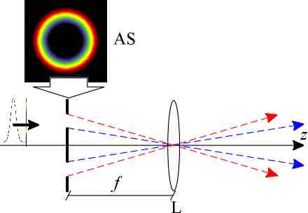
Figure 23: The principal scheme of a setup that generates optical FWM’s. Here L is a lens and AS is a chromatic angular slit. The angular dispersion arises as the consequence of the frequency dependence of diameter of the chromatic angular slit.

As an example of an alternative approach, characteristic in optics, consider a setup consisting of a Fourier lens of focal length $f$ and of a circularly symmetric mask with transfer function

$$t\left(R,k\right)=\emph{s}\left(k\right)\delta\left[R-f\tan\theta_{F}\left(k\right)\right]\text{,}$$ (233)

where $R$ is the radial coordinate on the ring and $\theta_{F}\left(k\right)$ is the angular function of a FWM defined by Eq. (34) – this is essentially an annular ring mask, the diameter of which depends on the wave number of the light as $R\left(k\right)=f\tan\theta_{F}\left(k\right)$ (see Fig. 23). It is well known, that each monochromatic point-source of wave number $k$ at some radial distance $\rho$ on the focal plane of an ideal the lens results in an apertured plane wave that subtends the angle $\theta_{F}\left(k\right)$ relative to $z$ axis behind the lens. The angular spectrum of plane waves of the total field then can be described as (here the infinite aperture is assumed)

$$A_{0}\left(k,\theta\right)=\emph{s}\left(k\right)\exp\left[i\upsilon\left(k\right)\right]\delta\left[\theta-\theta_{F}\left(k\right)\right]\text{,}$$ (234)

where $\upsilon\left(k\right)$ is some phase factor specific to the setup. The support of the angular spectrum of plane waves of the wave field is the one of the FWM’s (40). If we also compensate for the phase factor in Eq. (234) by applying the conjugated phase chirp to the input pulse the Fourier representation directly suggest that a transform-limited FWM can be generated by illuminating a ”chromatic” annular ring mask by a specifically chirped plane wave pulse. Though such chromatic mask is not very practical either, the advantage of this approach over the Gaussian aperture g10 in optical domain is obvious – this model is essentially static.

VI.2 Feasible approach to optical generation FWM’s

Let us introduce the general idea in terms of 2D FWM’s as defined in section III.3.1. Consider the pair of plane wave pulses propagating at angles $\theta_{0}$ and $-\theta_{0}$ relative to the optical axis (see Fig. 24a). Obviously we can introduce a tilt into their angular spectrum of plane waves by means of the angularly dispersive elements like diffraction gratings or prisms (wedges) and provided that the resulting tilted pulses overlap, we can observe the interference of two tilted pulses in near-axis conical volume [see the striped region in Fig. 24a]. If the introduced tilt of the plane wave components is such that the condition in the Eq. (34), i.e.,

$$\cos\theta_{F}\left(k\right)=\frac{\gamma\left(k-2\beta\right)}{k}$$ (235)

is satisfied for every $k$ and if we ignore for the while the diffractional edge effect that appear due to the finite aperture of the optical elements, the interference pattern in the near-axis volume is that of the 2D FWM.

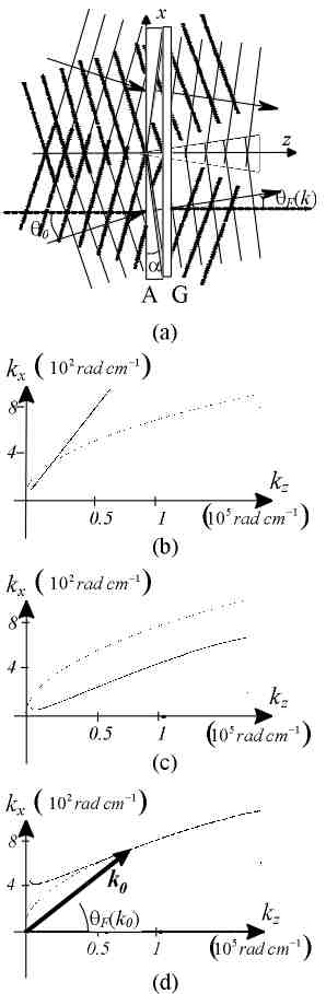
Figure 24: The general idea for optical generation of the 3D (2D) FWM’s: (a) The FWM generator consist of an axicon A and of circular diffractional grating G (or two wedges and linear diffractional grating respectively if we generate 2D FWM’s), the FWM can be observed in the conical volume (striped region) behind the diffraction grating; (b) The support of the angular spectrum of plane waves of the initial wave field on the FWM generator (solid line). Here and hereafter the dotted line denotes the support of angular spectrum of plane waves of the (2D) FWM under discussion, the dashed lines denote the bands of the frequency spectrum of the light used in our experiments (note the difference in scales between $k_{x}$ and $k_{z}$ axis); (c) The support of the angular spectrum of plane waves behind the axicon; (d) The support of the angular spectrum of plane waves at the exit of the FWM generator as compared with the theory.

The cylindrically symmetric case (FWM) can be considered similarly – one has to find the means to generate the superposition of Bessel beams, the support of the angular spectrum of which satisfies condition (235). Also, the use of the angular dispersion of the known generators of Bessel beams, i.e., the devices that transform a monochromatic plane wave into a Bessel beam, could be an appropriate idea.

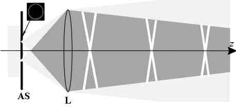
Figure 25: The Bessel–X pulse generator. Here L stands for lens and AS for angular slit.

As the first step we should generate the cylindrically symmetric counterpart of the pair of plane wave pulses – the Bessel–X pulse (see section IV.4.3). The general approach for this is quite straightforward – according to (133) we have to use the Bessel beam generator without any angular dispersion and illuminate it with a wideband pulse. The obvious choice is the annular slit in the back focal plane of a Fourier lens (see Fig. 25). The simple geometrical considerations show that in this case the wave field behind the lens is the cylindrically symmetric superposition of plane wave pulses – for the cone angle of the Bessel beam of the wave number $k$ we find $\sin\theta\left(k\right)=\sin\left(\arctan\left(D/f\right)\right)\equiv\sin\theta_{0}$, where $D$ is the diameter of the angular slit and $f$ is the focal length of the lens, so that the generated wave field can be approximated by (42)

$$\Psi_{BX}\left(\rho,z,t\right)=\int_{0}^{\infty}\mathrm{d}k\,\emph{s}\left(k\right)J_{0}\left(k\rho\sin\theta_{0}\right)\exp\left[ik\left(z\cos\theta_{0}-ct\right)\right]\text{,}$$ (236)

where $\emph{s}\left(k\right)$ is the frequency spectrum of the source field.

Using the Bessel-X pulses as input, the problem of optical generation of FWM’s reduces to the modeling of a set of diffractive elements that transform the conical support of the angular spectrum of plane waves so that the angular dispersion of the output pulse approximates the one described by the condition in Eq. (235) and to the ”compression” of the resulting wave field by compensating for the relative phases between its monochromatic components so that a transform-limited pulse appears on the optical axis.

There are various Bessel beam generators described in literature such as axicons, circular diffraction gratings, etc. (see, e.g., Ref. b1 – b16 and references therein). By illuminating those elements with a plane-wave pulse, we obviously get a superposition of Bessel beams, the support of the angular spectrum of which is determined by the wavelength dispersion of cone angle of the optical element $\theta\left(k\right)$. For example, an axicon is characterized by the complex transmission function $\exp\left[ik\tan\alpha\left(1-n\left(k\right)\right)\right]$, where $\alpha$ is the angle formed by the conical surface with a flat surface and $n\left(k\right)$ is the refractive index of the axicon (see, e.g., Ref. ba22 ). The method of stationary phase ok4 , applied as in Ref. ba15 , yields $\sin\theta\left(k\right)=\tan\alpha\left[1-n\left(k\right)\right]$. Hence, the angular spectrum of plane waves of the corresponding polychromatic wave field can be approximately described by

$$A_{0}\left(k,\theta\right)=\,\emph{s}\left(k\right)\delta\left[\theta-\arcsin\left(\tan\alpha\left(1-n\left(k\right)\right)\right)\right]\text{.}$$ (237)

Substitution into Eq. (17) yields

$$\Psi\left(\rho,z,t\right) =\int_{0}^{\infty}\mathrm{d}k~{}\emph{s}\left(k\right)J_{0}\left[k\rho\left(\tan\alpha\left(1-n\left(k\right)\right)\right)\right]$$ (238)

$$\times\exp\left[ik\left[z\cos\left(\arcsin\left(\tan\alpha\left(1-n\left(k\right)\right)\right)\right)-ct\right]\right]$$

and we can conclude that ideal Bessel beam generators can be used to design wave fields with cylindrically symmetric, two–dimensional supports of angular spectrum. Likewise, a circular grating yields for the cone angle $\sin\theta\left(k\right)=2\pi/kd$, where $d$ is the grating constant (first–order diffraction is assumed). The polychromatic wave field can be written as

$$\Psi\left(\rho,z,t\right) =\int_{0}^{\infty}\mathrm{d}k~{}\emph{s}\left(k\right)J_{0}\left[k\rho\left(\frac{2\pi}{kd}\right)\right]$$ (239)

$$\times\exp\left[ik\left(z\cos\left(\arcsin\left(\frac{2\pi}{kd}\right)\right)-ct\right)\right]$$

(note, that the Eqs. (238) and (239) do not count correctly for the longitudinal intensity change of Bessel beams behind axicons and circular diffraction gratings ba15 ; ba57 , they are brought about just to exemplify the use of the angular dispersion in our problem).

The support of angular spectrum of a FWM (34) cannot be approximated by a single diffractive element. However, we will show below that aside from the conventional configuration, where axicons and circular gratings are used to transform a plane wave into a Bessel beam, those elements can also be used to change the cone angle of Bessel beams. This property allows us to use a set of those Bessel beam generators as to design more complex supports of the angular spectrum.

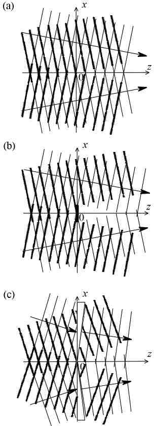
Figure 26: A qualitative description of a Bessel beam as a superposition of diverging (dotted lines) and converging (solid lines) conical waves in plane $z=0$ : (a) free–space evolution of the conical components; (b) diffraction on a circular opaque mask; (c) refraction on an axicon.

The generic features of the diffraction of Bessel beams on circularly symmetric optical elements can be understood by means of the following model. A zeroth–order Bessel function in the off–axis region can be well approximated by o2

$$J_{0}\left(a\right)\approx\frac{1}{2}\sqrt{\frac{2}{\pi a}}\left\{\exp\left[i\left(a-\frac{\pi}{4}\right)\right]+\exp\left[-i\left(a-\frac{\pi}{4}\right)\right]\right\}\text{.}$$ (240)

Substitution in (126) yields

$$\Psi_{B}\left(\rho,0,t\right) \approx\frac{1}{2}\sqrt{\frac{2}{\pi k\rho\sin\theta}}\left\{\exp\left[ik\rho\sin\theta-i\frac{\pi}{4}\right]\right.$$

$$+\left.\exp\left[-ik\rho\sin\theta+i\frac{\pi}{4}\right]\right\}\exp\left[-ikct\right]$$ (241)

for the Bessel beam  in plane $z=0$. In this expansion a Bessel beam in this plane is a superposition of two conical waves, as shown in Fig. 26a (see also Ref. b14 ). The evolution of those components can be qualitatively analyzed by means of ray–tracing, if we also recognize that the characteristic field distribution of a Bessel beam arises in the volume where the conical waves interfere. Typical examples, the free-space evolution and diffraction on circularly symmetric mask, are depicted in Fig. 26a and Fig. 26b. As one can see, such well-known features of Bessel beams as finite propagation length b1 and regeneration behind an opaque screen appear immediately.

Let us place an axicon (or circular grating) onto plane $z=0$ (see Fig. 26c). A qualitative analysis by means of ray-tracing immediately reveals, that the element changes the cone angle of both conical waves. The ”converging” conical wave forms a Bessel beam in a conical near axis volume, but the cone angle is now different. The ”diverging” conical component leaves the near axis region. Hence, axicons and diffraction gratings change the cone angle of a Bessel beam in the sense that the regenerated Bessel beam after the element is of a different cone angle.

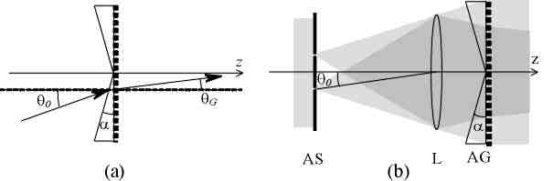
Figure 27: (a) A circular diffraction grating on the surface of an axicon – a composite optical element, which can be used for generation of FWM’s; (b) An optical setup for generation of FWM’s. A plane wave pulse is incident upon an annular slit (AS). Bessel–X pulse with cone angle $\theta$ behind a Fourier lens (L) is incident upon the composite optical element (AG).

Let us find the cone angle of the resulting Bessel beam for a composite optical element– a circular diffraction grating on the surface of an axicon (see Fig. 27a). We assume that a Bessel–X pulse with cone angle $\theta_{0}$, generated by means of an annular slit and Fourier lens, is incident upon it (see Fig. 27b). Snell’s law and the grating equation yield the following equation for the cone angle of the resulting Bessel beam:

$$\sin\theta_{G}\left(k\right)=\frac{2\pi}{kd}+n\left(k\right)\sin\left\{-\alpha+\arcsin\left[\frac{1}{n\left(k\right)}\sin\left(\theta_{0}+\alpha\right)\right]\right\}\text{.}$$ (242)

Here $d$ is the grating constant and $n\left(k\right)$ is the refractive index of the axicon material. Sign conventions are chosen so that the angles $\alpha$, $\theta_{0}$, $\theta_{G}\left(k\right)$ are positive in Fig. 27a. First–order diffraction is assumed. If the angles $\alpha$, $\theta_{0}$ are small, so that $\sin x\sim\arcsin x\sim x$, Eq. (242) yields

$$\theta_{G}\left(k\right)=\frac{2\pi}{kd}+\alpha\left[1-n\left(k\right)\right]+\theta_{0}\text{.}$$ (243)

Similar results can be obtained by means of the method of stationary phase. Below we use the approach in Ref. ba15 . Let the initial field on the diffractive element be the converging conical component of a Bessel beam $\frac{1}{2}\sqrt{2/\left(\pi k\rho\sin\theta_{0}\right)}\exp\left[ik\rho\sin\theta_{0}\right]$. The amplitude transmission function of the element is $\exp\left[ik\rho\left(2\pi/kd+\tan\alpha\left(1-n\left(k\right)\right)\right)\right]$. The corresponding Fresnel diffraction integral can be given as

$$\Psi\left(\rho,z\right)=\frac{1}{i\lambda z}e^{ik\left(z+\frac{\rho^{2}}{2z}\right)}\int\nolimits_{0}^{D}\mathrm{d}\rho^{\prime}f\left(\rho^{\prime}\right)\exp\left[ik\mu\left(\rho^{\prime}\right)\right]\text{,}$$ (244)

where

$$f\left(\rho^{\prime}\right)=\rho^{\prime}\frac{1}{2}\sqrt{\frac{2}{\pi k\rho^{\prime}\sin\theta_{0}}}2\pi J_{0}\left(\frac{k\rho\rho^{\prime}}{z}\right)$$ (245)

and

$$\mu\left(\rho^{\prime}\right)=\frac{\rho^{\prime 2}}{2z}-\rho^{\prime}\left(\frac{2\pi}{kd}+\tan\alpha\left(1-n\left(k\right)\right)+\sin\theta_{0}\right)\text{.}$$ (246)

The first derivative of $\mu\left(\rho^{\prime}\right)$ yields exactly one critical point $\rho_{c}^{\prime}$, namely

$$\rho_{c}^{\prime}=z\left(\frac{2\pi}{kd}+\tan\alpha\left(1-n\left(k\right)\right)+\sin\theta_{0}\right)\equiv z\sin\theta_{SP}\left(k\right)$$ (247)

and, according to Ref. ba15 , the leading contribution to (244) behaves as

$$\frac{1}{i\lambda z}\exp\left[ik\left(z+\frac{\rho^{2}}{2z}\right)\right]\int\nolimits_{0}^{D}\mathrm{d}\rho^{\prime}f\left(\rho^{\prime}\right)\exp\left[ik\mu\left(\rho^{\prime}\right)\right]\quad\quad\quad$$ (248)

$$\quad\quad\quad\quad\quad\quad\quad\quad\quad\quad\quad\quad\quad\approx\frac{1}{i\lambda z}\exp\left[ik\left(z+\frac{\rho^{2}}{2z}\right)\right]\frac{f\left(\rho_{c}^{\prime}\right)\exp\left[ik\mu\left(\rho_{c}^{\prime}\right)\right]}{\sqrt{k\mu^{\left(2\right)}\left(\rho_{c}^{\prime}\right)}}\text{,}$$

where $\mu^{\left(2\right)}\left(\rho_{c}^{\prime}\right)$ denotes the value of the second derivative $\mu\left(\rho_{c}^{\prime}\right)$ at the critical point. Substituting (247) into (248) and omitting some position-independent factors we get

$$\Psi\left(\rho,z\right) \approx\frac{1}{i\lambda z}\exp\left[ik\left(z+\frac{\rho^{2}}{2z}\right)\right]\frac{1}{\sqrt{k\frac{1}{z}}}z\sin\theta_{SP}\left(k\right)$$

$$\times\frac{1}{2}\sqrt{\frac{2}{\pi kz\sin\theta_{SP}\left(k\right)\sin\theta_{0}}}\left[2\pi J_{0}\left(\frac{k\rho z\sin\theta_{SP}\left(k\right)}{z}\right)\right]$$

$$\times\exp\left[ik\left(\frac{\left(z\sin\theta_{SP}\left(k\right)\right)^{2}}{2z}-z\sin^{2}\theta_{SP}\left(k\right)\right)\right]\text{,}$$ (249)

so that

$$\Psi\left(\rho,z\right)\sim J_{0}\left(k\rho\sin\theta_{SP}\left(k\right)\right)\exp\left[ik\frac{\rho^{2}}{2z}\right]\exp\left[ikz\cos\theta_{SP}\left(k\right)\right]\text{,}$$ (250)

where relation $1-\sin^{2}\theta/2\sim\sqrt{1-\sin^{2}\theta}=\cos\theta$ is used. We also have $k\left(\rho^{2}/2z\right)\ll\pi/2$ for the far–field in near–axis region and Eq. (249) reads

$$\Psi\left(\rho,z,t\right)\approx J_{0}\left(k\rho\sin\theta_{SP}\left(k\right)\right)\exp\left[ikz\cos\theta_{SP}\left(k\right)\right]\text{.}$$ (251)

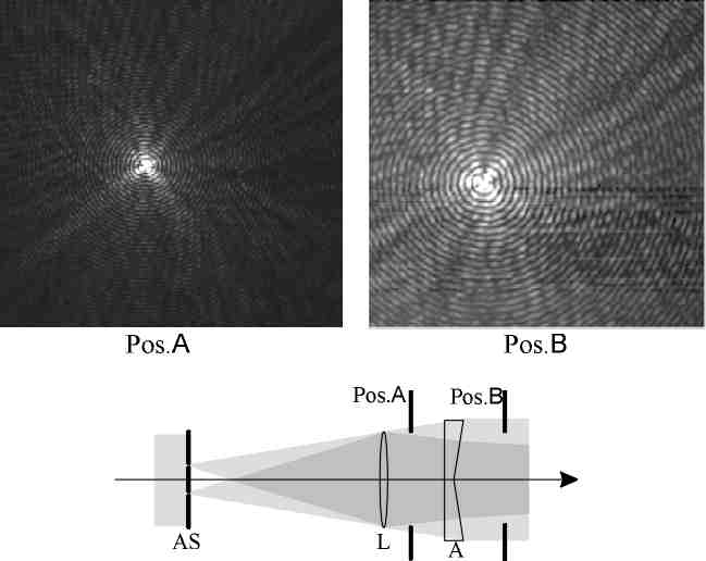
Figure 28: The experimental demonstration of the use of the angularly dispersive Bessel beam generators for change of the cone angle of monochromatic Bessel beams. In the setup: AS, annular slit; L, lens; A, ”hollow” axicon. In the left and right pane the CCD image of the Bessel beam at the plane A and B are depicted respectively.

Thus, the method of stationary phase yields a similar result as the qualitative ray tracing analysis – the output field of an axicon (or circular grating), illuminated by a Bessel beam, is a Bessel beam. If we assume a small angle limit i.e. $\sin x\sim\tan x\sim x$ in Eq. (247), the generated cone angle $\theta_{SP}$ is also exactly the same as predicted by the ray tracing analysis in Eq.(243) and we have shown that the Bessel beam generators can be used to change the cone angle of Bessel beams. We also carried out experimental proof of this principle, the typical results are depicted in Fig. 28.

The wavelength dispersion of the cone angle of the Bessel beam constituents of a FWM $\theta_{F}\left(k\right)$ is determined by Eq. (35). Combining this condition with the dispersion of the cone angle of the discussed setup $\theta_{G}\left(k\right)$ (243), we get

$$\arccos\left(\frac{\gamma\left(k-2\beta\right)}{k}\right)=\frac{2\pi}{kd}+\alpha\left(1-n\left(k\right)\right)+\theta_{0}\text{.}$$ (252)

In following chapters we will see that the three free parameters $\left(\alpha,\theta_{0},d\right)$ can be adjusted so that the relation (252) is satisfied in a very good approximation in a limited spectral range.

As to finish this section we note that care must be taken when specifying the frequency spectrum $B\left(k\right)$ or $\tilde{B}\left(k\right)=\allowbreak k^{2}\sin\theta\left(k\right)$ in Eqs. (234), (236), (237) and (239). In terms of the frequency spectrum of the light source $\emph{s}\left(k\right)$ – generally the choice the transform depends on the particular setup under consideration. If we set $\emph{s}\left(k\right)=\tilde{B}\left(k\right)$, we integrate over the monochromatic Bessel beams with amplitudes $\emph{s}\left(k\right)$. However, for example in the principal setup in Fig. 23 it is quite obvious that the amplitudes of the Bessel beams depend on the diameter of the annular slit – the larger diameter means larger area of the slit and more transmitted energy. Consequently, the ”chromatic” annular ring mask has a transfer function that is not constant but can be approximated by $\sim k\sin\theta\left(k\right)=\allowbreak\chi$ and one should use the weighting function $\tilde{B}\left(k\right)=\allowbreak k\sin\theta\left(k\right)\emph{s}\left(k\right)$ in the superposition over the Bessel beams or

$$\tilde{A}_{0}\left(k,\theta\right)=k\sin\theta\left(k\right)\emph{s}\left(k\right)\exp\left[i\upsilon\left(k\right)\right]\delta\left[\theta-\theta_{F}\left(k\right)\right]$$ (253)

in place of (234) for the angular spectrum of plane waves (here $\upsilon\left(k\right)$ stands for the phase distortions of the setup). As for the special cases of annular slit with constant diameter, axicon and circular diffraction grating the analogous arguments show that the replacement $\emph{s}\left(k\right)=\tilde{B}\left(k\right)$ applies. (note also how the otherwise exponential frequency spectrum of the FWM’s in Eq. (115) behaves as a Gaussian-like in (117) due to the $k\sin\theta_{F}\left(k\right)$ term in the expression of the Whittaker type plane wave expansion (17)). Of course, the generated wave field is propagation-invariant regardless of the weighting function in the superposition and generally in any optical experiment only the bandwidth of the source have to be concerned about.

VI.3 Finite energy approximations to FWM’s

We already noted in the overview in Chapter IV that the total energy content of FWM’s is infinite and as such they are not realizable in any physical experiment. We also referenced some of the most commonly used approaches to derive finite energy approximations to FWM’s. Obviously, in experimental situation a natural choice is to consider the approximations that correspond to the specific launching mechanism. In other words, the approximations of the type (152) should be given a physical content, in terms of limitations of a real experimental setup. In what follows we derive the finite energy approximation of FWM’s that is due to the finite aperture of the optical system introduced in previous chapter (Ref. m3 ).

In Fourier picture the starting point for this discussion is obvious. In this picture any realistic (finite-aperture) optical system generates a superposition of apertured monochromatic Bessel beams so that the field in the exit plane the FWM generator can be described by (for brevity we restrict ourselves to cylindrically symmetric case)

$$\Psi_{B}\left(\rho,0,0;k\right)=t\left(\rho\right)J_{0}\left[k\rho\sin\theta_{F}\left(k\right)\right]\text{,}$$ (254)

where $t\left(\rho\right)$ is the complex-amplitude transmission function of the aperture of the setup. One just has to show that (i) the resulting superposition of the apertured Bessel beams still represents a wave field that propagate as a FWM, and (ii) the superposition has finite energy content.

VI.3.1 Apertured (finite energy flow approximations to) Bessel beams

The simplest mathematical model for the monochromatic Bessel beams is the exact solution of the scalar homogeneous wave equation in Eq. (126)

$$\Psi_{B}\left(\rho,z,t\right)=J_{0}\left(k\rho\sin\theta_{0}\right)\exp\left[ik\left(z\cos\theta_{0}-ct\right)\right]\text{.}$$ (255)

In this case the beam can be described in Fourier’ picture by the single delta-ring in $k$-space and the transformation of the beam in free space and in optical elements can be easily estimated by simple geometrical constructions. However, such closed form Bessel beams are not square integrable. The most apparent approach to deduce physically realizable approximations to Bessel beams has been to apply a finite aperture to the system. The problem has been discussed in many works, mostly in terms of Fresnel approximation of scalar diffraction theory (see Refs. ba5 –ba82 and references therein).

As an alternative, we could use the Gaussian windowing profile and consider the paraxial wave equation – this combination yields a closed mathematical form of the beams, that have been called the Bessel-Gauss beams (see Refs. ba10 ; ba25 ; ba45 ; ba59 ; ba65 and references therein). However, the paraxial approximation lacks the physical transparency of the angular spectrum representation. Still, it should be noted, that the Bessel-Gauss beams can be used to construct wave fields that behave like LW’s propagating in free space.

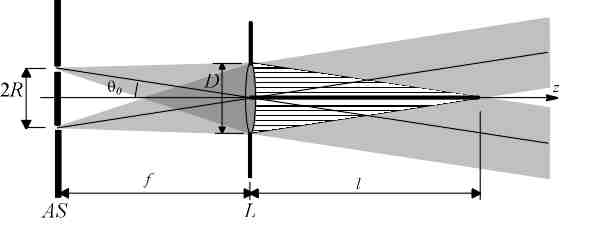
Figure 29: On the finite aperture approximations to the Bessel beams. The optical setup is the simple Bessel beam generator consisting of annular ring AS of diameter D, and the lens of aperture $D$ and focal length $f$. The striped region denotes the near axis volume where the generated wave field approximates closely the behaviour of the finite aperture Bessel beam.

We will use the generally accepted facts that (i) applying finite aperture to a Bessel beam provides us with a finite energy flow wave field, that is a very good approximation of the infinite-aperture Bessel beams (254) in a certain finite-depth, near axis volume (see, e.g., Ref. b2 ) and (ii) that the polychromatic superpositions of those apertured Bessel beams approximate very closely the superpositions of ”non-apertured” Bessel beams in this volume b14 . Such a behavior can be easily explained in the Fourier picture where a monochromatic Bessel beam is a cylindrically symmetric superposition of plane waves, that propagate at angle $\theta$ relative to $z$ axis. Indeed, as the apertured plane waves approximate their infinite aperture counterparts very closely in their central parts, one can also observe a very good approximation to the infinite-aperture Bessel beam in this near-axis volume (see striped region in Fig. 29 and Ref. ba62 for a more detailed description in terms of diffraction theory). If the cone angle of a Bessel beam is small, as it is always the case in paraxial optical systems, the apertured Bessel beam would behave as its infinite-aperture counterpart (254) for several meters of propagation.

The situation in Fig. 29 can be modeled by applying the transmission function $t\left(\rho\right)$ of the aperture to the Bessel beams. In Weyl picture this operation is equivalent to calculating the two-dimensional Fourier transform of the transversal amplitude distribution $t\left(\rho\right)J_{0}\left(\chi_{0}\rho\right)$, where $\chi_{0}$ stands for radial projection of the wave vector of the Bessel beam. Given the Weyl type angular spectrum of plane waves of the infinite-aperture Bessel beam

$$A\left(\chi\right)=K\delta\left(\chi-\chi_{0}\right)\text{,}$$ (256)

where $K$ is a constant, the Fourier transform of (254) in point $z=0$, $t=0$ can be found to be

$$A_{ApB}\left(\chi\right) =\frac{K}{\left(2\pi\right)^{2}}\,T\left(\chi\right)\ast\delta\left(\chi-\chi_{0}\right)$$

$$=\frac{\chi_{0}K}{\left(2\pi\right)^{2}}\int_{0}^{2\pi}\mathrm{d}\phi T\left(\sqrt{\chi^{2}+\chi_{0}^{2}-2\chi\chi_{0}\cos\left(\phi-\phi_{0}\right)}\right)\text{,}$$ (257)

where $T\left(\chi\right)$ is the two-dimensional Fourier transform of the transmission function $t\left(\rho\right)$ and $\ast$ denotes convolution operation (see also Ref. si25 ). The argument of the function $T\left({}\right)$ in (257) has an interpretation as being the distance between the points $\left(\chi,\phi\right)$ and $\left(\chi_{0},\phi_{0}\right)$. As for all convenient apertures the function $T\left(\chi\right)$ is well-localized around zero, the major contribution to the integral (257) comes from small values of $\phi$ and one can write in good approximation

$$A_{ApB}\left(\chi\right)\approx\frac{\chi_{0}K}{2\pi}T\left(\chi-\chi_{0}\right)\text{.}$$ (258)

The interpretation of the expression (258) is straightforward: the finite aperture gives the support of angular spectrum of a monochromatic Bessel beam a finite ”width”. Exact form of the support is determined by the complex-amplitude transmission function, however, the well-known set of fundamental Fourier transform pairs gives a good idea of what the support of angular spectrum looks like, without any calculations.

VI.3.2 Apertured FWM’s

First of all, it has been demonstrated both numerically and experimentally that the superposition of apertured Bessel beam behaves like the superposition of their infinite-aperture counterpart in near-axis volume as defined in Fig. 29. Thus we can claim that the substitution of infinite-aperture Bessel beams in (40) by their apertured counterparts should generate a finite energy flow wave field that is a good approximation of the FWM (42) in this finite volume. In other words, in this near-axis volume the apertured wave field can be well approximated by the formulas of infinite-aperture wave fields.

Obviously, the finite aperture has a similar effect on the angular spectrum support of a FWM – the delta function in Eq. (40) is substituted by a weighting function and the angular spectrum of plane waves of apertured FWM’s can be written as

$$A_{ApF}\left(k,\chi\right) =\frac{\chi_{F}\left(k\right)B\left(k\right)}{\left(2\pi\right)^{2}}\int_{0}^{2\pi}\mathrm{d}\varphi$$

$$\times T\left(\sqrt{\chi^{2}+\chi_{F}\left(k\right)^{2}-2\chi\chi_{F}\left(k\right)\cos\varphi}\right)$$

$$\approx\frac{\chi_{F}\left(k\right)B\left(k\right)}{2\pi}T\left[\chi-\chi_{F}\left(k\right)\right]\text{,}$$ (259)

where $\chi_{F}\left(k\right)=k\sin\theta_{F}\left(k\right)$. Consequently, the Weyl type plane wave expansion of the wave field behind the aperture reads

$$\Psi_{ApF}\left(\rho,z,t\right) =\int_{0}^{\infty}\mathrm{d}k\int_{0}^{\infty}\mathrm{d}\chi\,\chi\,A_{ApF}\left(k,\chi\right)$$

$$\times J_{0}\left(\rho\chi\right)\exp\left[ik\left(z\sqrt{k^{2}-\chi^{2}}-ct\right)\right]\text{.}$$ (260)

Alternatively, the transformation $\chi=k\sin\theta$ gives the expression (260) the following form

$$\Psi_{ApF}\left(\rho,z,t\right) =\int_{0}^{\infty}\mathrm{d}kk^{2}\int_{0}^{2\pi}\mathrm{d}\theta\sin\theta\cos\theta\,A_{ApF}\left(k,k\sin\theta\right)$$

$$\times J_{0}\left(k\rho\sin\theta\right)\exp\left[ik\left(z\cos\theta-ct\right)\right]\text{.}$$ (261)

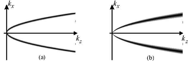
Figure 30: The comparison of the supports of angular spectrums of plane waves of (a) an apertured FWM and (b) of an EDEPT type superposition of FWM’s as described in above sections.

The support of the angular spectrum of plane waves (259) of the derived wave field is depicted on Fig. 30a. In correspondence with Eq. (258) it has a finite ”thickness”. We can outline the main difference between the support of angular spectrum of LW’s, proposed in this section (261) and that of EDEPT’s (152) discussed in section IV.6.1. The comparison of their supports of angular spectrum of plane waves on Fig. 30a and 30b (respectively) shows, that the transversal ”width” in $k_{x}k_{y}$ plane of angular spectrum of plane waves of our apertured FWM’s is a constant– such a result is a consequence of applying aperture with a wavelength-independent complex-amplitude transmission function. On the other hand, the transversal width is generally not constant for the superpositions of FWM’s in Eq.(152). The description in this section gives the property a straightforward interpretation: the corresponding aperture has a wavelength dependent complex-amplitude transmission function. In the context of our discussion, where the main goal is optical feasibility, such an approach should be regarded as an impractical one.

The spatial localization of the result (260) can be estimated by the approach in section III.1.5 – obviously the resulting wave field still has the characteristic narrow central peak. Also, in correspondence with the note in the beginning of current section, the field of apertured and non-apertured FWM’s do not differ noticeably in the near-axis volume at $t=0$. Thus, if the aperture of the system is reasonably large (several millimeters) the only qualitative effect of the finite aperture is the reduced propagation length of the wave field.

There is several ways to estimate the propagation length of the apertured FWM’s. The simplest possibility is still use the geometrical construction in Fig. 29 from which we can write

$$l_{1}\left(k_{\min}\right)=\frac{D}{2\tan\left[\theta_{F}\left(k_{\min}\right)\right]}\text{,}$$ (262)

where $k_{\min}$ denotes the minimal wave vector of the spectrum of the wave field (note, that for the supports of FWM’s this generally corresponds to maximum angle $\max\left[\theta_{F}\left(k\right)\right]$, i.e., to the minimal propagation length of the corresponding Bessel beams [clarify Fig. 29)]. The second possibility is to estimate the propagation length of the apertured monochromatic Bessel beams by means of the approach in the section III.1.5 (in present case where the wave field is essentially monochromatic, this is actually the McCutchen theory as introduced in Ref. mc5 ). From the Eq. (76) we at once get

$$l_{2}\left(k_{\min}\right)=\Delta z=\frac{\Delta\rho}{\tan\theta_{F}\left(k_{\min}\right)}\text{,}$$ (263)

i.e., we get identical result as in Eq. (262). The third possibility is to estimate the maximum group- and phase velocity uncertainty of the finite width support of the angular spectrum of plane waves (257).

In conclusion, in our setup the finite energy (physically realizable) approximations to FWM’s are introduced quite plainly by the finite aperture of the optical system. In Fourier domain this corresponds to smoothing of the delta function in the angular spectrum of plane waves of the wave fields. Also, the double integrals in Eq. (260) can in some detail be handled without excessive numerical calculations.

VI.3.3 On finite time window excitation of the FWM’s

In literature, there has been several works on generation of FWM’s where the finite total energy has been achieved by limiting the excitation time of the source array g4 ; g5 ; g6 ; g10 . It has been shown, that, indeed, such approach do not destroy the localized propagation of the generated pulses. It is intuitively clear, that the finite time excitation results in a superposition of the longitudinal ”fragments” of the monochromatic Bessel beams. In this picture the reasonable time window indeed do not corrupt the behaviour of the central part of the wave field, and it is still a good approximation that of the exact monochromatic Bessel beam. What the time window do is that it broadens the frequency spectrum of the points of the source matrix. Correspondingly, the support of the angular spectrum of the generated wave field would look much like the one in Fig. 30a. Actually, the excitation time of our setup is also finite and the two broadening effects – due the aperture and the finite excitation time – appear simultaneously, however, the one that is caused by the finite aperture is several orders of magnitude stronger.

VI.4 Optical generation of partially coherent LW’s

The direct comparison of the equations describing the angular spectrum of plane waves of coherent and partially coherent LW’s in Eqs. (33) – (45) and (192) – (195) respectively implies, that the main part of the generating setup should be the same for both cases. Indeed, the partially coherent quasi-monochromatic plane waves transform in linear optical systems similarly as the coherent monochromatic plane waves, at least the description of the previous chapter concerning refraction and diffraction in grating hold for both cases. The qualitative difference lies in the correlations between the plane wave components.

VI.4.1 The light source

According to our general idea of the optical generation of FWM’s in Sec. VI.2, we need a well-directed wideband partially coherent plane wave as the initial field in our setup. In mathematical limit the angular spectrum of plane waves of such initial field is described by

$$a(\phi,\theta,k)=s(k)\delta\left[\theta\right]\text{,}$$ (264)

giving for the field

$$V(\mathbf{r},t)=\frac{1}{2\pi}\int_{0}^{\infty}\mathrm{d}k\ s(k)\exp\left[ik\left(z-ct\right)\right]\text{,}$$ (265)

where $s\left(k\right)$ is generally stochastic function. Such field is fully coherent in transversal direction. In longitudinal direction the coherence time $\tau_{c}$ is determined by the bandwidth of the light $\Delta k$ and the reciprocity inequality ok4

$$\tau_{c}\Delta k\geq\frac{1}{2c}\text{.}$$ (266)

For the ensemble average, we can write

$$\left\langle s^{\ast}(k_{1})s(k_{2})\right\rangle=\mathcal{S}\left(k\right)\delta\left(k_{2}-k_{1}\right)\text{,}$$ (267)

where $\mathcal{S}\left(k\right)$ denotes the spectral density (power spectrum) of the light source so that the mutual coherence function reads as

$$\Gamma\left(\Delta z,\tau\right)=\int_{0}^{\infty}\mathrm{d}k\mathcal{S}\left(k\right)\exp\left[ik\left(\Delta z-c\tau\right)\right]\text{.}$$ (268)

In other words, the mutual coherence function of light field behaves like a plane wave pulse of the duration $\tau_{s}$ in coherent optics.

The traditional approach to generate such field is to use a thermal light source, for example the superhigh-pressure Xe-arc lamp, and spatially filter the light by means of a pinhole. The well-known drawback of the choice is the hugely reduced signal level as compared to laser sources. The alternative is to use a directional white-light continuum source.

VI.4.2 FWM’s with frequency noncorrelation

As it was explained in section V.2.2 (clarify Eqs. (209) and (210)), the FWM’s with frequency noncorrelation differ from their fully coherent counterparts only by the lack of correlation between the fluctuations of their Fourier components of different frequency. Obviously such fields can be generated by illuminating the setup in Fig. 27b with a wideband partially coherent plane wave as described in Eqs. (264) – (268).

VI.4.3 FWM’s with angular noncorrelation

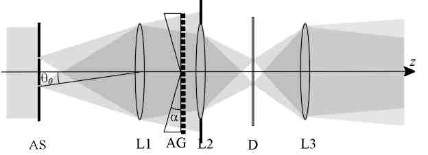
Figure 31: The principal setup for generation of FWM’s with angular noncorrelation: AS, annular slit; L1, L2, L3, lenses; AG, annular grism; D, diffuser;

According to section V.2.3 the only difference between the fully coherent FWM’s and this special case is the lack of correlation between the tilted pulses that compose the coherent FWM’s. Thus, to generate a FWM with angular noncorrelation one has to illuminate the setup by coherent light and somehow break the correlation between the tilted pulses propagating at different polar angles. This can be done by means of the modified setup depicted in Fig. 31 (see Ref. ok6 for the description of corresponding quasi-monochromatic case). In this setup the pair of lenses L2, L3 is inserted into the path of FWM’s so that in the focal plane of L2 the two-dimensional Fourier transform of the FWM’s – the characteristic concentric rings – appear. In this plane we can insert a weak diffuser as to modify the amplitude and phase of the tilted pulses.

VI.4.4 FWM’s with frequency and angular noncorrelation

In this special case one has to illuminate the setup in Fig 31 with the white-light source as described in Eqs. (264) – (268).

VI.5 Conclusions. Optical generation of general LW’s

As to conclude this chapter we note that except for the ultra-wide bandwidths, required to generate the wave fields described in Chapter IV the concept of propagation-invariance is well realizable in optical domain – we have shown, that the angular dispersion of various Bessel beam generators can be used to transform the support of the angular spectrum of plane waves so that to approximate that of the FWM’s in some limited near-axis volume. The choice of the combination of the elements may be a problem in some cases, however, the chances are good for finding satisfactory combination. Consequently, one can launch the wave fields with the characteristic central peak that propagates over reasonable distances.

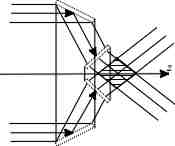
Figure 32: Optical generation of LW’s that contain plane waves that subtend non-paraxial angles with respect to the optical axis.

Note, that the LW’s containing plane waves that propagate at nonparaxial relative to $z$-axis can in principle be generated within the framework of this approach. Nevertheless, this requires very non-conventional optical elements like conical mirrors and diffraction gratings as sketched in Fig. 32. Also, in this case the propagation distance of the generated LW’s is quite short as can be seen from Eq. (262).

VI.6 On the physical nature of propagation-invariance of pulsed wave fields

As to conclude the theoretical part of this review we interpret some of the properties of the LW’s in the context of classical diffraction theory (see Ref. x49k for a relevant discussion).

The first note has to be made on the definition of the propagation length of LW’s. Namely, it has been claimed in several publications (see Ref. g0a for example) that the LW’s propagate over extended distances as compared to that, defined by the Rayleigh range $Z_{R}$, the well known estimate for the scale length of the falloff in intensity behind of a Gaussian aperture in the diffraction theory, defined as (see Ref. o25 for example)

$$Z_{R}=\frac{\pi W_{0}^{2}}{\lambda}\text{,}$$ (269)

$W_{0}$ being the minimum spot size (radius) of the beam. Indeed, for the apertured FWM’s the radial diameter of its central spot is approximately (75)

$$d\approx\frac{4.81}{k_{0}\sin\theta_{F}\left(k_{0}\right)}=1.5\times 10^{-4}m$$

(again, $\gamma=1$, $\beta=40\frac{rad}{m}$) and if we consider a planar source with diameter $D=1cm$, this spot travels (262)

$$l_{1}\left(k_{\min}\right)=\frac{D}{2\tan\left[\theta_{F}\left(k_{\min}\right)\right]}=0.9m\text{,}$$ (270)

The Rayleigh range (269) of the Gaussian pulse with radius $W_{0}=d$ is $Z_{R}\approx 8.8cm\allowbreak\ll l_{1}\left(k_{\min}\right)$. However, in our opinion such estimates are misleading and should not be used without the following additional details.

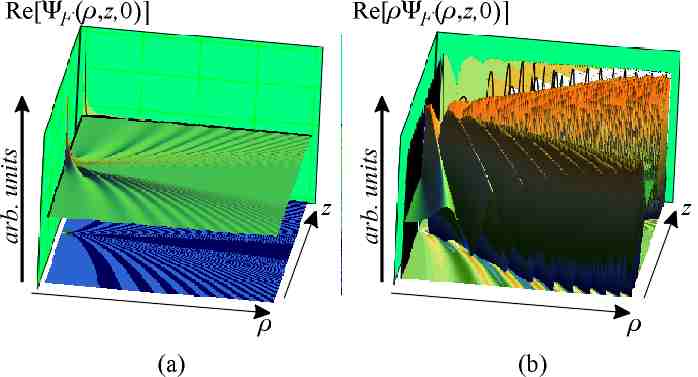
Figure 33: The comparison of the radial field distribution of a FWM (left pane) with the field that is integrated over the polar angle (right pane).

The effect of diffraction is typically manifested when an obstacle is placed in the path of a light field. For (pulsed) beams the definition (269) determines minimal spread corresponding to the waist radius $W_{0}$. In other words, this parameter determines the minimum radius of a circular aperture that can be placed in the path of the beam without significantly distorting its behaviour behind the aperture. Now, as to compare the two estimates we have to ask, what is the waist radius of an apertured FWM’s?

It appears, that the situation is similar to that with the monochromatic Bessel beams for which the energy content in every transverse lobe is approximately constant and equal to the energy content in the central maximum (see Ref. x49k for example). In the case of apertured FWM’s the amplitude of the branches of the characteristic X-shape fall off approximately as $1/\rho$. Thus, the integrated energy density as the function of radial coordinate $\rho$ is approximately constant, as the integration over the polar angle adds the factor $\rho$ to the amplitude of the wave field (see Fig. 33). Thus, only a minor part of the energy of the apertured FWM’s is contained in its central lobe and if one has to compare the propagation length of the apertured FWM’s with the Rayleigh range of the Gaussian pulses, one should take $W_{0}=D$ instead of $W_{0}=d$ in (269).

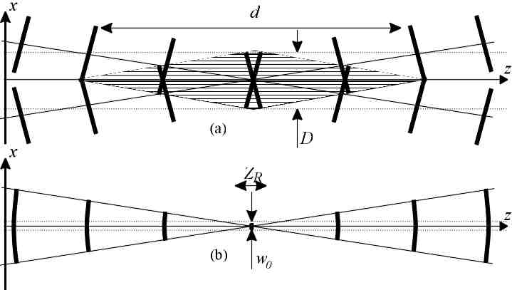
Figure 34: The comparison of the focusing of (a) FWM’s and (b) Gaussian pulses (see text).

As the matter of fact, such comparison of the Gaussian pulse and apertured FWM’s is not appropriate as focusing of the two wave fields are of qualitatively different physical nature. Namely, the Gaussian pulses are composed of monochromatic components with curved phase fronts, the phase fronts of the monochromatic components of the FWM’s are conical. In lights of this difference, one can say that the FWM’s are never focused in the conventional sense of the term and the term, focus wave mode, is rather misleading.

In focusing Gaussian pulses most of its energy content can be concentrated into a single spot for a time moment. A cunning mental picture of the energetic propertied of focusing in FWM’s can be acquired if we suppose that we have an ideal (apertured) FWM generator and suppose that we illuminate it with a plane wave pulse. Then central peak of each monochromatic Bessel beam component of the generated FWM’s has the amplitude equal to the amplitude of the corresponding monochromatic plane wave component of the initial plane wave pulse. Indeed, the effect of the FWM generator to this monochromatic plane wave component is that its initial energy in the $k$-space (a finite width spot on the $k_{z}$-axis) is smeared over the finite width toroid in the $k$-space. In real space each point in this toroid will compose an apertured plane wave in the Bessel beam and the net on-axis amplitude of the Bessel beam is the integrated amplitude over the toroid in $k$-space, i.e., again the amplitude of the initial monochromatic plane wave component. Now, for the superposition of the Bessel beams we can say, that the only place where the constructive interference occurs is the central spot of the apertured FWM. Thus, we can say, that given the initial plane wave pulse with the amplitude $A$ and aperture $D$, the amplitude of the central spot of an apertured FWM behind an ideal FWM generator is that of the initial plane wave pulse $A$, the rest of the energy is in the sidelobes of the generated FWM’s. This consequence is a good illustration of the qualitative difference between the FWM’ and Gaussian pulse – due to the curved phase fronts of its monochromatic components the latter can indeed effectively transfer most of its energy to a single spot for a time moment.

VII THE EXPERIMENTS

In our experiments we realized the optical setups for two LW’s – the apertured Bessel-X pulses and apertured FWM’s and used an interferometric cross-correlation method with time-integrated intensity recording to study the generated wave fields. The material of this chapter is published in Refs. I and V.

VII.1 FWM’s in interferometric experiments

A straightforward method for recording the complicated field shape of a coherent FWM or Bessel-X pulses would use a CCD camera with a gate in front of it, which should possess a temporal resolution and a variable firing delay both in subfemtosecond range. As such a gate is not realizable, any workable idea of experiment has to resort to a field cross-correlation technique (see Refs. ok7 –ok17 and references therein).

In our experiments the wave field under investigation $F\left(\mathbf{r},t\right)$ interfere with a reference wave $V_{P}$:

$$V_{\Sigma}\left(\mathbf{r},t\right)=F\left(\mathbf{r},t\right)+V_{P}\left(\mathbf{r},t\right)\text{.}$$ (271)

For the reference wave we can write

$$V_{P}\left(\mathbf{r},t\right)=\int_{0}^{\infty}\mathrm{d}k\,\emph{s}\left(k\right)\upsilon_{P}\left(k\right)\exp\left[ik\left(z-c\left(t+\Delta t\right)\right)\right]\text{,}$$ (272)

where $\emph{s}\left(k\right)$ is the (generally stochastic) frequency spectrum of the light source, $\upsilon_{P}\left(k\right)$ is the spectral phase shift introduced by the optics in the reference arm of the interferometer, $\left|\upsilon_{P}\left(k\right)\right|\equiv 1$ and $\Delta t$ denote the variable time delay between the signal and reference wave fields. For the wave field under investigation we have

$$F\left(\mathbf{r},t\right)=\int_{0}^{\infty}\mathrm{d}k\,\emph{s}\left(k\right)\,\upsilon_{F}\left(k\right)J_{0}\left[kx\sin\theta_{F}\left(k\right)\right]\exp\left[ik\left(z\cos\theta_{F}\left(k\right)-ct\right)\right]\text{,}$$ (273)

where $\upsilon_{F}\left(k\right)$ is again the undesirable spectral phase shift from the setup, $\left|\upsilon_{F}\left(k\right)\right|\equiv 1$ (we have assumed here that the FWM generator transform the input light so that for every spectral component $\emph{s}\left(k\right)$ the amplitude of the central spot of the corresponding Bessel beam is also $\emph{s}\left(k\right)$). The averaged intensity of the resulting wave field can be expressed as

$$\left\langle V_{\Sigma}^{\ast}V_{\Sigma}\right\rangle=\left\langle V_{P}^{\ast}V_{P}\right\rangle+\left\langle F^{\ast}F\right\rangle+2\operatorname{Re}\left\langle F^{\ast}V_{P}\right\rangle$$ (274)

(here the exact meaning of the angle brackets depends on the statistical properties of the light source of the experiment).

The quantities $\left\langle V_{P}^{\ast}V_{P}\right\rangle$ and $\left\langle F^{\ast}F\right\rangle$ denote time-independent intensity of the wave field. Specifically, the first term in the sum is the uniform intensity of the plane wave pulse:

$$\left\langle V_{P}^{\ast}V_{P}\right\rangle=\int_{0}^{\infty}\mathrm{d}k\mathcal{S}\left(k\right)\text{,}$$ (275)

where again $\mathcal{S}\left(k\right)=\left\langle\emph{s}^{\ast}\left(k\right)\emph{s}\left(k\right)\right\rangle$ is the spectral density. The second term is the time-averaged intensity of $F$:

$$\left\langle F^{\ast}F\right\rangle=\int_{0}^{\infty}\mathrm{d}k\mathcal{S}\left(k\right)J_{0}^{2}\left[kx\sin\theta_{F}\left(k\right)\right]\text{.}$$ (276)

In principle the two components can be eliminated from the results by recording them separately and by numerically subtracting them from the interferograms.

From Eqs. (272) and (273) we can write

$$2\operatorname{Re}\left\langle F^{\ast}V_{P}\right\rangle=2\operatorname{Re}\left\langle\int_{0}^{\infty}\mathrm{d}k_{1}\emph{s}^{\ast}\left(k_{1}\right)\upsilon_{F}^{\ast}\left(k_{1}\right)\right.$$

$$\qquad\qquad\times J_{0}\left(k_{1}\rho\sin\theta_{F}\left(k\right)\right)\exp\left[-ik_{1}\left(z\cos\theta_{F}\left(k\right)-ct\right)\right]$$

$$\qquad\qquad\times\left.\int_{0}^{\infty}\mathrm{d}k_{2}\emph{s}\left(k_{2}\right)\upsilon_{P}\left(k_{2}\right)\exp\left[ik_{2}\left(z-c\left(t-\Delta t\right)\right)\right]\right\rangle\text{.}$$ (277)

In our discussion we concentrated on two limiting special cases of the classification in Sec. V.2 – the fully coherent LW’s (section V.2.1) and the LW’s with frequency noncorrelation (section V.2.2). In both cases the averaging in (277) yields

$$\left\langle F^{\ast}V_{P}\right\rangle=\int_{0}^{\infty}\mathrm{d}k\,\mathcal{S}\left(k\right)\upsilon_{F}^{\ast}\left(k\right)\upsilon_{P}\left(k\right)$$

$$\qquad\times J_{0}\left(kx\sin\theta_{F}\left(k\right)\right)\exp\left[ikz\left(\cos\theta_{F}\left(k\right)-1\right)+ikc\Delta t\right]\text{.}$$ (278)

Here for the partially coherent field we have used Eq. (267):

$$\left\langle\emph{s}^{\ast}\left(k_{1}\right)\emph{s}\left(k_{2}\right)\right\rangle=\mathcal{S}\left(k_{1}\right)\delta\left(k_{1}-k_{2}\right)\text{,}$$ (279)

for coherent fields the $\delta\left(k_{2}-k_{1}\right)$ appears as the time-averaging over the term $\exp\left[ict\left(k_{2}-k_{1}\right)\right]$. Equation (278) can be given the form

$$\left\langle F^{\ast}V_{P}\right\rangle=\exp\left[i2\beta\gamma z\right]\int_{0}^{\infty}\mathrm{d}k\,\mathcal{S}\left(k\right)\upsilon_{F}^{\ast}\left(k_{1}\right)\upsilon_{P}\left(k\right)$$

$$\qquad\quad\times J_{0}\left(k\rho\sin\theta_{F}\left(k\right)\right)\exp\left\{ik\left[z\left(1-\gamma\right)-c\Delta t\right]\right\}\text{.}$$ (280)

The above mathematical description yields identical results for the coherent and partially coherent fields, i.e., the results of such experiments generally do not depend on the correlations between the Fourier components of different frequency of the wave fields – it is well known that in any interferometric experiment the phase information of wave fields is necessarily lost. In other words, the results of the experiments do not depend on whether we use the transform-limited femtosecond pulses or a source of a stationary white noise.

The latter consequence is of great practical significance. In our overview in Chapter IV we used a spectrum that corresponds to a $3fs$ laser pulse and showed that the corresponding FWM’s and Bessel-X pulse had a good spatial localization (see Fig. 13 and 17). However, computer simulations, or even simple geometrical estimations show that if the autocorrelation time of the source field $\tau$ exceeds $\sim 10$ femtoseconds, the characteristic X branching occurs too far from the axis $z$ and in this narrow-band limit the resulting wave field would be nothing but a trivial interference of quasi-monochromatic plane waves. Thus, the bandwidth of the light source is a very challenging part of the setup. In what follows we add to the reputation of incoherent sources as being the poor mans femtosecond source and confine ourselves to the special case of frequency non-correlating fields.

VII.2 Experiment on optical Bessel-X pulses

VII.2.1 Setup

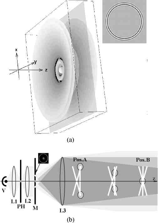
Figure 35: (a) Intensity profile of a computer-simulated Bessel-X pulse flying in space, shown as surfaces on which the field intensity is equal to a fraction $0.13\left(1/e^{2}\right)$ of its maximum value in the central point. The field intensity outside the central bright spot has been multiplyed by the radial distance in order to reveal the weak off-axis side-lobes. Inset: amplitude distribution in the plane shown as intersecting the pulse. The plots have been computed for 3-fsec near-Gaussian-spectrum source pulse with carrier wavelenght $\lambda=0.6\mu m$ and the angle $\theta_{0}=0.223\deg$. For these parameters the dimensions of the plot $xyz$ box are 20 times 20 times $\mu m$; (b) Optical scheme of the experiment. Mutual instantaneous placement of the Bessel-X pulse and the plane wave pulse is shown for three recording positions (two of which labeled in accordance with Fig. 36). The ovals indicate toroid-like correlation volumes where co-propagating Bessel-X and plane wave pulses interfere at different propagation distances along the $z$-axis. L’s, lenses; M, mask with Durnin’s annular slit and an additional central pinhole for creating the plane wave; PH, cooled pinhole $10\mu m$ in diameter to assure the transversal coherence of the light from the source V. In case source V generates a non-transform-limited pulses or a white cw noise, the bright shapes depict propagation of the correlation functions instead of the pulses.

Our setup for the interferometric experiments on optical Bessel-X pulses is depicted in Fig. 35b – as compared to the Bessel-X pulse generator in Fig. 25 the pinhole is made in the centre of the annular ring mask as to form the reference field (plane wave pulse) behind the lens L. For the mathematical description of the situation we have to choose $\beta=0$ in Eq. (280), i.e., $\theta\left(k\right)\equiv\theta_{0}=\allowbreak\arccos\gamma=\arccos c/v$. Setting also $\Delta t=0$ we get

$$\left\langle F^{\ast}V_{P}\right\rangle =\int_{0}^{\infty}\mathrm{d}k\mathcal{S}\left(k\right)\upsilon_{F}^{\ast}\left(k_{1}\right)\upsilon_{P}\left(k\right)$$

$$\times J_{0}\left(k\rho\sin\theta_{0}\right)\exp\left[ikz_{m}\left(1-\gamma\right)\right]$$ (281)

where $\mathcal{S}\left(k\right)$ is the spectral density of the light source (note that the annular ring mask has the uniform spectral response function as explained in the end of the Sec. VI.2). In Eq. (281) $z_{m}$ denotes the distance along the optical axis of the setup. To understand the significance of this parameter we have to remember the superluminal group velocity of the Bessel-X pulse – during the flight the latter catch-up with the reference plane wave pulse. In this context the coordinate $z_{m}$ is the distance of the recording device from this catch-up point (see Fig. 35b).

If we define in the general expression for the mutual coherence function of the wave fields in Eq. (216) the origin of the $z$ axis as being in the point $z=ct$ so that $\Delta z$ can be replaced by the distance from the pulse centre $z_{\Delta}$ and set $\tau=0$, $\mathbf{r}_{\bot 1}\equiv\mathbf{r}_{\bot}$, $\mathbf{r}_{\bot 2}=0$ the result reads

$$\Gamma_{F}\left(\mathbf{r}_{\bot},0,z_{\Delta}\right)=\exp\left[i2\beta\gamma z_{\Delta}\right]\int_{0}^{\infty}\mathrm{d}k\left|\mathcal{V}\left(k\right)\right|^{2}J_{0}\left(k\rho\sin\theta_{F}\left(k\right)\right)\exp\left[ik\gamma z_{\Delta}\right]\text{.}$$ (282)

If we also set $\beta=0$ we get

$$\Gamma_{BX}\left(\mathbf{r}_{\bot},0,z_{\Delta}\right)=\int_{0}^{\infty}\mathrm{d}k\left|\mathcal{V}\left(k\right)\right|^{2}J_{0}\left(k\rho\sin\theta_{0}\right)\exp\left[ik\gamma z_{\Delta}\right]\text{.}$$ (283)

Comparing the Eqs. (281) and (283) we see that if $\left|\mathcal{V}\left(k\right)\right|^{2}=\allowbreak\mathcal{S}\left(k\right)$ and $\upsilon_{F}^{\ast}\left(k_{1}\right)\upsilon_{P}\left(k\right)\allowbreak\equiv 1$, we have

$$\left\langle F^{\ast}V_{P}\right\rangle=\Gamma_{BX}\left(\mathbf{r}_{\bot},0,z_{m}\frac{1-\gamma}{\gamma}\right)\text{,}$$ (284)

so that

$$z_{\Delta}=z_{m}\frac{1-\gamma}{\gamma}\text{.}$$ (285)

The interpretation of the small factor $\left(1-\gamma\right)/\gamma$ in (285) is that the setup serves as a ”$z$ axis microscope” for recording the mutual coherence function (281) along the $z$-axis which scales the micrometer-range $z$ dependence of the field into a centimeter range.

If we compare the expression (283) with the hypothetically measurable field distribution given as the real part of the Bessel-X pulse in Eq. (135),

$$\Psi_{BX}\left(\rho,z,t\right)=\int_{0}^{\infty}\mathrm{d}k~{}\emph{s}\left(k\right)J_{0}\left[k\rho\sin\theta_{0}\right]\exp\left[ik\left(z\gamma-ct\right)\right]$$ (286)

we conclude that the experiment reveals the whole spatiotemporal structure of the Bessel-X field. The natural price we have to pay for resorting to the correlation measurements is replacing the spectrum $\emph{s}\left(k\right)$ with its autocorrelation, which is a minor issue in the case of transform-limited source pulses. Nevertheless, we cannot claim, that we actually detect the field under investigation (see also Ref. m1 for a relevant discussion). Indeed, as the absolute phases of the plane wave components are inevitably lost in any linear interferometric experiments only the spatial amplitude distribution of the wave field can be detected.

In the reasons described above we took advantage of the insensitivity of Eq. (281) to the source field phase and used a white light noise from a superhigh pressure Xe-arc lamp instead of a laser as the field source to achieve the $\sim 3$ femtosecond correlation time in our experiment (V in Fig. 35b). Thus we implemented the third special case of Sec. V.2 – the Bessel-X field with frequency noncorrelation.

VII.2.2 Results of the experiment

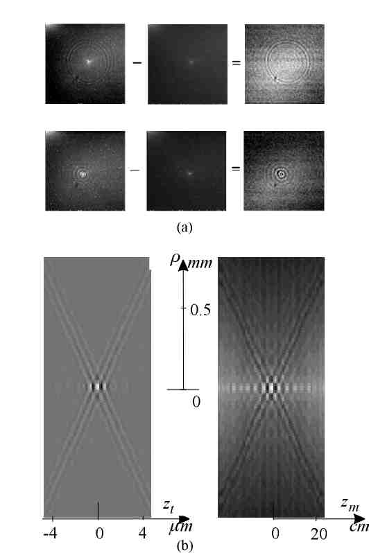
Figure 36: (a) Samples of the experimental recordings and processing of the intensity distributions measured at the positions Pos.A and Pos.B along the $z$-axis as shown in Fig. 35b. Left column, total interference pattern of the cross-correlated fields; middle column, lateral intensity distribution of the Bessel-X field alone. In the right column gray (about 50 per cent) corresponds to zero level and dark to negative values; (b) Comparison of the result of the experiment (right panel) with a computer-simulated Bessel-X pulse field.

The recordings at 70 points on the $z$ axis (from behind the L3 lens up to a point a few centimeters beyond the origin) with a 0.5-cm step were performed with a cooled CCD-camera EDC–1000TE, which has $2.64\times 2.64~{}mm$ working area containing $192\times 165$ pixels, and processed by a PC as follows.

First, the subtraction of the Bessel-X field intensity was performed (see Fig. 36a), whereas the same procedure with the plane wave field intensity, due to its practically even distribution, was found to be unnecessary. In order to reduce noise and the dimensionality of the data array, an averaging over the polar angle in every recording was carried out by taking advantage of the axial symmetry of the field. Thus we got a 1D array containing up to hundred significant elements from every $192\times 165$ matrix recorded. Seventy such arrays formed a matrix, which, having in mind the known symmetry of the real part of Eq. (281), was mirrored in the lateral and the axial plane. The result is compared in Fig. 36b with the Bessel-X field distribution in an axial plane, computed from Eq. (286) for a model spectrum. The latter was taken as a convex curve covering the whole visible region from blue to near infrared (up to $0.9~{}\mu m$) in order to simulate the effective light spectrum in the experiment, which is a product of the Xe-arc spectrum and the sensitivity curve of the camera. The central (carrier) frequency was chosen corresponding to wavelength $0.6~{}\mu m$ which had been determined from the fringe spacing of an autocorrelation pattern recorded for the light source with the same CCD camera. The left- and right-hand tails of the central X-like structure are more conspicuous in the experimental pattern due to unevenness of the real Xe-arc spectrum. The different scaling of the horizontal axes of the two panels is in accordance with the $z$ axis ”magnification” factor of the experimental setup.

Observing the obvious agreement between theoretical and experimental patterns, we arrive at a conclusion that we have really recorded the characteristic spatiotemporal profile of an optical realization of the nonspreading axisymmetric Bessel-X field.

VII.3 Experiment on optical FWM’s

VII.3.1 3D FWM’s and 2D FWM’s, the mathematical description of the experiment

To prove the feasibility of the approach for optical generation of apertured FWM’s described in Chapter VI one has to implement the setup depicted in Fig. 27b and show that the generated wave field indeed behaves as a FWM in interferometric experiments. However, without the loss of generality the task can be simplified as follows.

In section III.3.1 we demonstrated that all the defining properties of the FWM’s – its propagation-invariance, the characteristic field distribution and pre-determined group velocity – can be studied in terms of the specific pair of interfering tilted pulses, the 2D FWM’s in Eq. (89):

$$F_{2D}\left(x,y,z,t\right)=\int_{0}^{\infty}\mathrm{d}k\,\tilde{B}\left(k\right)$$

$$\qquad\qquad\times\cos\left[kx\sin\theta_{F}\left(k\right)\right]\exp\left[ik\left(z\cos\theta_{F}\left(k\right)-ct\right)\right]$$ (287)

(here we have set $\phi=0$). In other words, we have shown that the peculiar propagation of FWM’s is assured exclusively by the specific coupling between the wave number and the direction of propagation of plane wave components of the FWM’s as defined by the function $\theta_{F}\left(k\right)$ in Eq. (34).

In m5 we experimentally demonstrated the feasibility of 2D FWM’s in Eq. (287) as the physical concept which is much more transparent in this sort of experiments. However, it also appeared, that the fabrication and polishing of a high-quality, large aperture concave conical surfaces is still a complicated task.

The mutual coherence function for the 2D FWM’s can be easily deduced from the one for the (3D) FWM’s (216). In complete analogy with the discussion in section III.3.1 we replace the Bessel function $J_{0}\left({}\right)$ by $\cos\left({}\right)$, choose appropriate coordinates and get

$$\Gamma_{2D}\left(x_{1},x_{2},\Delta z,\gamma\Delta z-c\tau\right)=\exp\left[-i\beta\gamma\Delta z\right]\int_{0}^{\infty}\mathrm{d}k~{}\left|\mathcal{V}\left(k\right)\right|^{2}$$

$$\quad\qquad\times\cos\left(kx_{1}\sin\theta_{F}\left(k\right)\right)\cos\left(kx_{2}\sin\theta_{F}\left(k\right)\right)\exp\left[ik\left(\gamma\Delta z-c\tau\right)\right]\text{.}$$ (288)

Also, the mathematical description of the experiments with 2D FWM’s is analogous to that of the three-dimensional one. In the spatial intensity distribution of the interferometric experiment

$$\left\langle V_{\Sigma}^{\ast}V_{\Sigma}\right\rangle=\left\langle V_{P}^{\ast}V_{P}\right\rangle+\left\langle F_{2D}^{\ast}F_{2D}\right\rangle+2\operatorname{Re}\left\langle F_{2D}^{\ast}V_{P}\right\rangle\text{,}$$ (289)

we have for the intensity of the 2D FWM

$$\left\langle F_{2D}^{\ast}F_{2D}\right\rangle=\int_{0}^{\infty}\mathrm{d}k\mathcal{S}\left(k\right)\cos^{2}\left(kx\sin\theta_{G}\left(k\right)\right)$$ (290)

where the angular function $\theta_{G}\left(k\right)$ [see Eq. (242)] is determined by the specific setup and $\mathcal{S}\left(k\right)$ is the spectral density of the light source (see notes in the end of the Sec. VI.2). For the third term instead of Eq. (280), we have

$$\left\langle F_{2D}^{\ast}V_{P}\right\rangle =\exp\left[2\beta\gamma z\right]\int_{0}^{\infty}\mathrm{d}k\,\mathcal{S}\left(k\right)\upsilon_{F}^{\ast}\left(k_{1}\right)\upsilon_{P}\left(k\right)$$

$$\times\cos\left(k\rho\sin\theta_{G}\left(k\right)\right)\exp\left\{ik\left[z\left(1-\gamma\right)-c\Delta t\right]\right\}\text{.}$$ (291)

In (291) for FWM’s we have to set $\gamma=1$, so that

$$\left\langle F_{2D}^{\ast}V_{P}\right\rangle =\exp\left[2\beta z\right]\int_{0}^{\infty}\mathrm{d}k\mathcal{S}\left(k\right)\upsilon_{F}^{\ast}\left(k_{1}\right)\upsilon_{P}\left(k\right)$$

$$\times\cos\left(k\rho\sin\theta_{G}\left(k\right)\right)\exp\left[-ikc\Delta t\right]\text{.}$$ (292)

In analogy with the case of Bessel-X fields we can define in (288) $\Delta z=0$, $\mathbf{r}_{\bot 2}=0$, so that the mutual coherence functions of the 2D FWM reads

$$\Gamma_{2D}\left(x,0,0,-c\tau\right)=\int_{0}^{\infty}\mathrm{d}k~{}\left|\mathcal{V}\left(k\right)\right|^{2}\cos\left(kx\sin\theta_{G}\left(k\right)\right)\exp\left[-ikc\tau\right]\text{.}$$ (293)

Thus, if we record the interference pattern at $z=0$, the comparison of Eqs. (293) and (291) yields

$$\left\langle F_{2D}^{\ast}V_{P}\right\rangle_{\Delta t}=\Gamma_{2D}\left(x,0,0,-c\Delta t\right)\text{,}$$ (294)

and we can conclude that the mutual coherence function of the 2D FWM’s can be studied by recording the intensity of the interference picture as the function of the delay $\Delta t$ between the signal and reference fields.

Note, that the equation (292) can be given the form

$$\left\langle F_{2D}^{\ast}V_{P}\right\rangle=\int_{0}^{\infty}\mathrm{d}k\mathcal{S}\left(k\right)$$

$$\qquad\times\cos\left(kx\sin\theta_{G}\left(k\right)\right)\exp\left[ikz\cos\theta_{G}\left(k\right)-ikc\left(t_{0}-\Delta t\right)\right]\text{,}$$ (295)

where $t_{0}=z/c$ and the constant has the interpretation of being the time that a wave field propagating at group velocity $c$ travels the distance $z$ to the plane of measurement. The integral expression (295) is very similar to the one describing the field of the 2D FWM’s (287), the only difference being that the theoretical angular function $\theta_{F}\left(k\right)$ is replaced by the $\theta_{G}\left(k\right)$ and frequency spectrum is replaced by the power spectrum $\mathcal{S}\left(k\right)$ in (295). Again, as the absolute phases of the plane wave components are inevitably lost in any linear interferometric experiments we can detect only the amplitude distribution of the wave field. However, the interferograms do carry information about the defining, most essential characteristic of the FWM’s – their support of the angular spectrum of plane waves. Indeed, the general structure of the interference patterns in Eq. (295) is primarily determined by the angular function $\theta_{G}\left(k\right)$, and it resembles the corresponding transform-limited wave field only if $\theta_{G}\left(k\right)=\allowbreak\theta_{F}\left(k\right)$ in good approximation over the entire bandwidth of the field.

VII.3.2 Setup

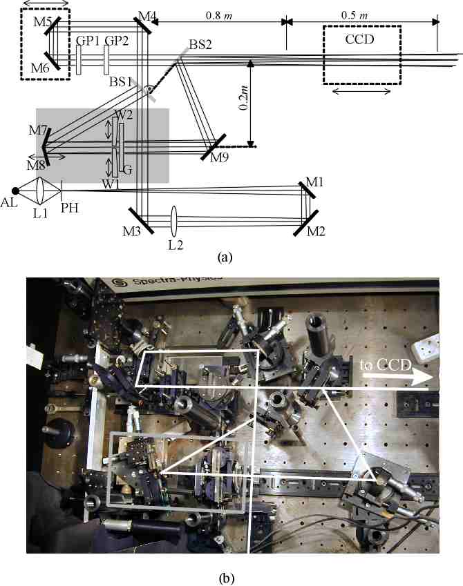
Figure 37: Experimental setup for generating 2D FWM’s and recording its interference with plane wave pulses. The FWM generator can be seen in grayed area; M’s, mirrors; L’s, lenses; BS’s, beam splitters; W’s, wedges; G, diffractional grating; AL, Xe-arc lamp; PH, pinhole; GP’s, compensating glass plates.

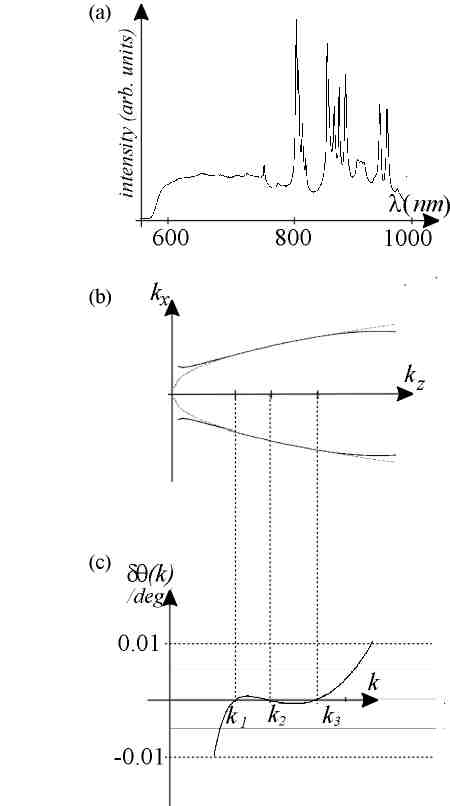
Figure 38: (a) The power spectrum of the light used in our setup; (b) The angular spectrum of the plane waves generated in the setup (solid black line) as compared to the theoretical one (dotted cyan line); (c) The deviation of generated support, here $k_{1}=7.4\times 10^{6}\frac{rad}{m}$ ($\lambda=849nm$), $k_{2}=10.6\times 10^{7}\frac{rad}{m}$ ($\lambda=593nm$), $k_{3}=1.6\times 10^{7}\frac{rad}{m}$ ($\lambda=381nm$).

The conversion of the FWM generator in Fig. 27b to the two-dimensional case is straightforward – we just replace the axicon and circular diffraction by their one-dimensional counterparts – prisms (wedges) and a diffraction grating. The initial field on the elements is an interfering pair of pulsed plane waves.

The setup of our experiment is depicted in Fig. 37. The main part of it is the (2D) FWM generator that consist of the mirrors M7 and M8, of the two wedges W1 and W2 and of a blazed diffraction grating G.(see grayed area in Fig. 37). The FWM generator is placed into an arm of an interferometer as will be explained below.

In our experiment we implemented a 2D FWM with following parameters: $\beta=\allowbreak 40rad/m$, $\gamma=1$ ($v_{g}=c$) giving $\theta_{F}\left(k_{0}\right)\approx\allowbreak 0.23{{}^{\circ}}$ if $k_{0}=\allowbreak 7.8\times 10^{6}rad/m$ ($\lambda_{0}\approx 800nm$) (see Fig. 38a for the spectral density of the light source and Fig. 38b for the support of the angular spectrum of plane waves of the specified 2D FWM).

The FWM generator has three free parameters: $\alpha$ – the apex angle of the wedges, $\theta_{0}$ – the angle that the initial pulsed plane waves subtend with the optical axis of the setup and $d$ – the groove spacing of the diffraction grating. As to find the values for the parameters that give the best fit between the generated support of the angular spectrum of plane waves and the support of angular spectrum of plane waves of the theoretical FWM’s in Eq. (34)

$$\theta_{F}\left(k\right)=\arccos\left(\frac{k-2\beta}{k}\right)$$ (296)

($\gamma=1$) we combine the (296) with the Eq. (243) and write the following system of equations:

$$\arccos\left(\frac{\gamma\left(k_{m}-2\beta\right)}{k_{m}}\right)=\frac{2\pi}{k_{m}d}+\alpha\left(1-n\left(k_{m}\right)\right)+\theta_{0}\;,m=1,2,3\text{.}$$ (297)

We specify the three wave numbers as $k_{1}=7.4\times 10^{6}\frac{rad}{m}$ ($\lambda=849nm$), $k_{2}=10.6\times 10^{7}\frac{rad}{m}$ ($\lambda=593nm$), $k_{3}=1.6\times 10^{7}\frac{rad}{m}$ ($\lambda=381nm$) and assumed that the wedges are made of the optical glass BK 7 for which the refractive index $n\left(k\right)$ is known to an accuracy better than $10^{-5}$. The system (297) then yields

$$\alpha =1.2044\times 10^{-2}rad$$

$$d =3.7494\times 10^{-4}m$$ (298)

$$\theta_{0} =9.4683\times 10^{-3}rad~{}\text{.}$$

As inserted into Eq. (242), the maximum deviation $\delta\theta\left(k\right)=\theta_{F}\left(k\right)-\theta_{G}\left(k\right)$ for the wavelength dispersion of the cone angle in the selected spectral range is as small as $5\times 10^{-4}\deg$, i.e., $<0.2\%$. A comparison of the corresponding supports of angular spectrum and the exact form of deviation $\delta\theta\left(k\right)$ are depicted in Figs. 38b and 38c (see also Fig. 24). As for rough estimation of the spread of the pulse due to the $\delta\theta\left(k\right)$ one can estimate the corresponding maximum group velocity dispersion $\Delta v^{g}$ and compare this with the mean wavelength of the pulse. The numerical simulations show that the approximation is indeed good enough for propagating the central peak of the FWM’s over several meters.

The FWM generator has been placed in what is basically a specially designed, modified Mach-Zehnder interferometer. The interferometer consists of two beamsplitters and of identical broadband non-dispersive mirrors. The input field from the light source is split by the beamsplitter BS1 into the fields that travel through the two arms of the interferometer, the one with the FWM generator and the arm for the reference beam. The mirrors M5 and M6 form a delay line, they were translated by the Burleigh Inchworm linear step motor, the $1\mu m$ translation step of which was reduced to $65nm$ by a transmission mechanism. The mirror M7 was continuously translatable as to correct for the time-shift between the two tilted pulses. The wedges W1 and W2 were transversally translatable as to balance the material dispersion they introduce to the plane wave pulses (see text below). We used Kodak Megaplus 1.6i CCD camera with the $1534\times 1024$ matrix resolution and 10 bit pixel depth. The linear dimensions of the matrix are $13.8mm$(H)$\times 9.2mm$(V), the pixel size is $9\mu m\times 9\mu m$.

Again, in our experiment we used the filtered light form a superhigh pressure Xe-arc lamp, giving $\approx 5\,fsec$ correlation time for the input field [see Fig. 38a for the power spectrum of the light]. To ensure good transversal coherence over the clear aperture of the setup the required maximum diameter $\approx 15\mu m$ of the pinhole and focal length $2m$ of the collimating Fourier lens L1 was estimated from the van Cittert-Zernike theorem ok4 for the mean wavelength of the light $\lambda_{0}=800nm$. As the result of filtering, the total power of the signal on the $\approx 1.5cm^{2}$ CCD chip was very low, approximately $0.03\mu W$.

Due to the short coherence time of the source field, the experiment is highly sensitive to the phase distortions (spectral phase shift) introduced by the dispersive optical elements of the system – the beamsplitters and the FWM generator. In the FWM generator there is three possible sources of undesirable dispersion: (1) the propagation in the glass substrate of the diffraction grating, (2) the propagation between the grating and the axicon where the support of angular spectrum of the wave field is not appropriate for the free space propagation, i.e., it does not obey the Eq. (34) and (3) the propagation in the wedges. The beamsplitters in our setup are identical and if we set them perpendicularly and orient the coated sides so that each beam passes the glass substrate of the beamsplitter twice, the arms of the interferometer remain balanced. The influence of the propagation between the elements can be made neglible by placing them close to each other. The character of the undesirable dispersion in the wedges can be estimated from the following considerations. The entrance wave field on the wedges is the transform-limited Bessel-X pulse, so, the on-axis part of the pulse is also transform-limited and should pass through the wedges unchanged, i.e., without any additional spectral phase shift. Consequently, the wedges should be produced and aligned so that their thickness is zero on the optical axis. As the apex angle of the wedges is very small in our setup ($\approx 0.7{{}^{\circ}}$), this is not very practical approach and we consider the finite thickness on the axis as the source of additional spectral phase shift instead. Thus, the composite spectral phase shift of the FWM generator can be described as the phase distortion introduced by the substrate of the diffraction grating and by a glass plate of the material of the wedges, the thickness of which is equal to the thickness of the wedges on the optical axis. We balanced the arms of the interferometer by inserting material dispersion into the reference arm of the setup by means of two appropriate glass plates (GP1 and GP2 in Fig. 37a).

VII.3.3 Results of the experiment

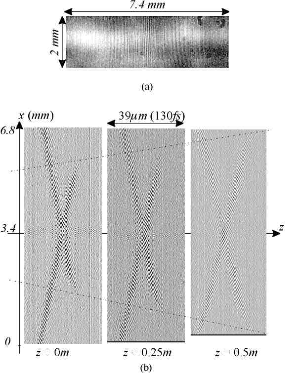
Figure 39: (a) A typical interferogram in the setup as recorded by the CCD camera; (b) The interference pattern in the setup as the function of the delay between the signal and reference wave fields in three positions of the CCD camera (see text for more detailed description).

In first experiment we recorded the time-averaged interference pattern of the 2D FWM and the reference wave field as the function of the time delay between the two. The experiment can be mathematically modeled by varying parameter $\Delta t$ in Eq. (292). We scanned the time-delay at three $z$-axis positions, $z=0cm$, $z=25cm$, $z=50cm$ (the origin of the $z$-axis is about $30cm$ away from the beamsplitter BS2 in Fig. 37a). In each experiment we recorded $300$ interferograms, the time-delay step was $0.43\,fsec$ ($0.13\,\mu m$).

In a typical interference pattern in our experiment [see Fig. 39a] the sharp vertical interference fringes in the center correspond to the second term in the interference sum (289) – this is the time-averaged, ”propagation-invariant” time-averaged intensity of the 2D FWM. The fringes can also be interpreted as the autocorrelation function of the interfering tilted pulses [see Fig. 38a for the corresponding power spectrum]. In this experiment the intensity of the wave field under study do not carry any important information, so we subtracted it numerically from the results in Fig. 39b. The interference fringes that are symmetrical at both sides of the central part correspond to the third, most important term in this sum. It can be seen from Fig. 39a, that due to the low signal level the recorded interferograms are quite noisy. To get the better signal-to-noise ratio, we averaged the data in the interferograms over the rows and used the resulting one-dimensional data arrays instead.

The results of the experiment are depicted in Fig. 39b. We can see, that there is a good qualitative resemblance between the measured $x\Delta t$ plot of the interference pattern and the theoretical field distribution of the 2D FWM’s in Fig. 7b as it was predicted by the Eq. (295) – one can clearly recognize the two interfering tilted pulses forming the characteristic X-branching, also the phase fronts in the tilted pulses can be seen. The wave field is definitely transform-limited, so we have managed to compensate for the spectral phase shift in the 2D FWM generator.

We can also see, that the interference pattern does not show any spread over the $0.5\,m$ distance, consequently, the wave field does not spread in the course of propagation.

An additional detail can be found in Fig. 39b: the tilted pulses do not extend across the whole picture but are cut out (see dashed lines in Fig. 39b). Also, the ”edges” of the tilted pulses move away from the optical axis. This effect can be clearly interpreted as the consequence of the finite extent of the tilted pulses, as illustrated in Figs. 24a and 26 – the dashed lines simply mark the borders of the volume, where the two tilted pulses intersect, i.e., the borders of the volume, where the 2D FWM exist [see the striped area in Fig. 24a].

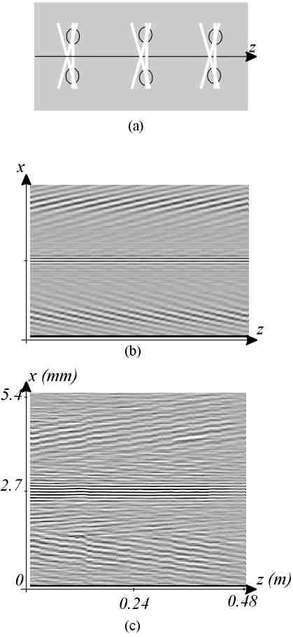
Figure 40: The interference pattern as the function of the CCD camera position (see text for detailed description).

In the second experiment we recorded the interference pattern as the function of the propagation distance $z$. The experiment can be simulated by varying $z$ coordinate in Eq. (292). We recorded $240$ interferograms, the step of the CCD camera position was $3.1\,mm$. The numerical simulation of the experiment and the results of the experiment are depicted in Figs. 40b and 40c respectively.

The experiment can be easily interpreted – the position-invariant envelope of the interference pattern is the consequence of the fact, that the group velocities of the propagation-invariant 2D FWM and the reference field are equal, $c$, so that the overlapping volume of the two fields do not change in the course of propagation (see Fig. 40a). The $z$ dependent finer structure of the interferograms is the consequence of the fact, that the phase velocities of the plane wave pulse and 2D FWM are not equal, i.e., we have also $v^{g}\neq v^{p}$ for the phase and group velocities of the 2D FWM. The result of the experiment in Fig. 40c show good qualitative agreement with the theory.

We can also determine the parameter $\beta$ from our experiment – the exponent multiplier in Eq. (292) reads $\exp\left[i2\beta z\right]$, thus $\beta=\pi/z_{0}$ where $z_{0}$ is the period of the variations along the $z$-axis. From the result in Fig. 40a we estimated $z_{0}\approx 7.5cm$, so that $\beta\approx 42\,rad/m$, which result is in good agreement with the theory.

Thus, we have shown, that the generated wave field has all the characteristic properties described in previous theoretical sections and the validity of the general idea has been given an experimental proof.

VIII SELF-IMAGING OF PULSED WAVE
FIELDS

Self-imaging, also known as Talbot effect is, in its original sense, a well-known phenomenon in classical wave optics where certain wave fields reproduce their transversal intensity distribution at periodic spatial intervals in the course of propagation (see Refs. si1 – si30 , and references therein). The effect has been studied extensively by means of Fresnel diffraction theory and the angular spectrum representation of scalar wave fields. As a result, the general, physically transparent conditions have been formulated the transversal intensity distribution of a wave field have to obey to be self-imaging. It is also well known that the monochromatic propagation-invariant wave fields (Bessel beams) constitute a special class of self-imaging wave fields, the mathematical description of the two being much the same.

In recent years the effect has attracted a renewed interest, as the concept has been generalized into the domain of pulsed wave fields by several authors (see Refs. si20 ; si28 ; si29 ; si37 ; si40 , and references therein). The phenomenon has been discussed in the context of fiber optics si20 and also as a property of spatial, wideband wave fields si28 ; si29 ; si37 ; si40 .

In what follows we show, that the discrete superpositions of FWM’s over the parameter $\beta$

$$\Psi^{\left(SI\right)}\left(\rho,z,\varphi,t\right)=\sum_{q}C_{q}\Psi_{F}\left(z,\rho,\varphi,t;\beta_{q}\right)$$ (299)

can be used as the self-imaging “pixels” of a spatiotemporally self-imaging three-dimensional spatial image – the wave fields of this type can reproduce spatial separated copies of its initial three-dimensional intensity distribution at specific time intervals. The results in this chapter are published in Ref. m4 .

(It is important to note, that our discussion is closely related to those in Refs. [si28 ] and si40 – those publications consider essentially the same problem, however the analysis is different in each occasion)

VIII.1 Monochromatic self-imaging

The self-imaging condition for the monochromatic wave field has been defined as (see, e.g., Ref. si10 )

$$\Psi\left(\rho,z,\varphi,t\right)=\Psi\left(\rho,z+d,\varphi,t\right)\text{.}$$ (300)

With the condition (300) and the Whittaker type angular spectrum of plane waves of monochromatic wave fields (see Eq. (17)

$$\Psi\left(\rho,z,\varphi,t;k\right) =\sum_{n=0}^{\infty}\exp\left[\pm in\varphi\right]\int_{0}^{\pi}\mathrm{d}\theta\mathbf{~{}}\tilde{A}_{n}\left(k,\theta\right)$$

$$\times J_{n}\left(k\rho\sin\theta\right)\exp\left[ik\left(z\cos\theta-ct\right)\right]$$ (301)

one can easily deduce the condition for self-imaging for the monochromatic scalar wave fields that reads si10

$$kd\cos\theta=\psi+2\pi q\text{,}$$ (302)

where $q$ is an integer and $\psi$ is an arbitrary phase factor. The relation (302) implies, that a monochromatic wave field (15) periodically reconstructs its initial transversal field distribution if only its angular spectrum of plane waves is sampled so that the condition

$$k_{z}=\frac{\psi+2\pi q}{d}\text{,}$$ (303)

where $k_{z}$ is again the $z$ component of the wave vector, is satisfied for every plane wave component of the wave field. Applying the condition (303) and including only the axially symmetric terms in the summation, we get the following expression for the general cylindrically symmetric, monochromatic, self-imaging wave field:

$$\Psi\left(\rho,z,t;k\right)=\exp\left[-i\omega t\right]\sum_{q}a_{q}J_{0}\left[k\rho\sqrt{1-\left(\frac{2\pi q}{d}\right)^{2}}\right]\exp\left[i\frac{2\pi q}{d}z\right]\text{,}$$ (304)

where we have denoted

$$a_{q}=\tilde{A}_{0}\left(k,\arccos\frac{2\pi q}{kd}\right)$$ (305)

and $\psi=0$ is assumed. Thus, we have a discrete superposition of Bessel beams the cone angles are specified by Eq. (303). The physical content of Eqs. (303) and (304) can be summarized by saying that the monochromatic self-imaging is essentially the phenomenon where the wave field is a discrete superposition of wave fields with different phase velocities so that the total field, being the superposition of the composite fields, depends periodically on the distance.

The on-axis superposition in (304),

$$\Psi\left(\rho,z,t;k\right)=\exp\left[-i\omega t\right]\sum_{q}a_{q}\exp\left[i\frac{2\pi q}{d}z\right]$$ (306)

can be recognized as the Fourier series representation of a periodic function along the optical axis. However, in (306) the condition (302) together with the causality requirement $k_{z}>0$ imply that

$$0<q<\frac{kd}{2\pi}\text{.}$$ (307)

An example of the on axis intensity distribution of a superposition of Bessel beams in (306) is depicted in Fig. 43.

VIII.2 Self-imaging of pulsed wave fields

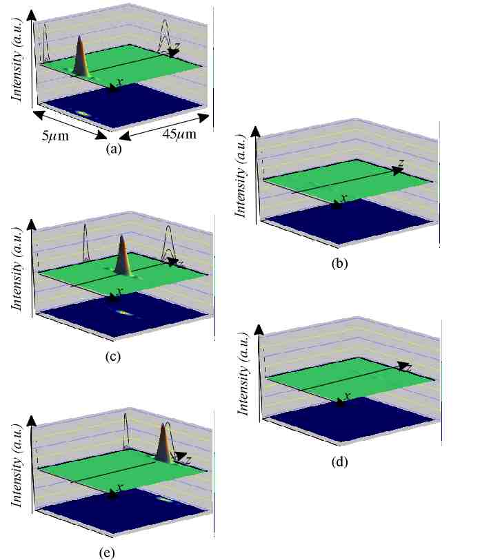
Figure 41: The snapshots of the temporal evolution of the spatial intensity distributions of the pulsed self-imaging wave field, the three-dimensional self-imaging “pixel”, at 26 femtosecond time intervals. Due to the axial symmetry, the distribution is shown in one meridional (say, $xz$) plane.

From the material in Chapter III we know that the phase velocities $v^{p}$ of the FWM’s with different parameter $\beta$ along the optical axis are generally different and we can write

$$v^{p}\left(\beta\right)=\frac{c}{\cos\theta_{F}\left(k_{0},\beta\right)}=\frac{ck_{0}}{\gamma\left(k_{0}-2\beta\right)}\text{.}$$ (308)

Thus, the superposition of FWM’s over the parameter $\beta$ in (299)

$$\Psi^{\left(SI\right)}\left(\rho,z,\varphi,t\right)=\sum_{q}C_{q}\Psi_{F}\left(z,\rho,\varphi,t;\beta_{q}\right)$$ (309)

is taken over a set of overlapping, non-spreading optical pulses that (1) are transversally localized, i.e., their transversal intensity distribution have a single narrow intense peak, (2) have equal carrier frequency, (3) propagate at equal group velocities, but (4) have different phase velocities. In complete analogy with the monochromatic self-imaging we could suggest that if the component pulses satisfy certain conditions, the single narrow peak of the wave field could periodically vanish and reconstruct its initial (localized) transversal intensity distribution. As a result we could get a wave field the temporal evolution of which can be perceived as a spatial arrow of sequentially visible light spots (see Fig. 41). In this sense, such superposition could be considered self-imaging and, due to its spatial localization, it could be used as a pulsed “self-imaging pixel” of a transversal or even spatial image.

Consider a discrete superposition of a set of the tilted pulses in Eq. (88)

$$T^{\left(SI\right)}\left(x,z,t\right)=\sum_{q}a_{q}\int_{0}^{\infty}\mathrm{d}k\,\tilde{A}\left(k\right)\exp\left[ik\left(x\sin\theta_{F}\left(k\right)+z\cos\theta_{F}\left(k\right)-ct\right)\right]\text{,}$$ (310)

the function $\theta_{F}\left(k,\beta_{q}\right)$ being determined by the Eq. (34). The expression can be given a readily interpretable form if we approximate the $x$ and $z$ components of the wave vector by

$$k_{x}\left(k,\beta\right)=k_{x}\left(k_{0},\beta\right)+\left.\frac{d}{dk}k_{x}\left(k,\beta\right)\right|_{k=k_{0}}\left(k-k_{0}\right)$$ (311)

$$k_{z}\left(k,\beta\right) =k_{z}\left(k_{0},\beta\right)+\left.\frac{d}{dk}k_{z}\left(k,\beta\right)\right|_{k=k_{0}}\left(k-k_{0}\right)$$

$$=k_{z}\left(k_{0},\beta\right)+\gamma\left(k-k_{0}\right)\text{,}$$ (312)

where we have used Eq. (33). Substitution of relations (311) and (312) in Eq. (310) yields

$$T^{\left(SI\right)}\left(x,z,t\right)\cong\sum\limits_{q}a_{q}L_{q}\left(x,z\gamma-ct\right)$$

$$\qquad\times\exp\left[ik_{0}\left(x\sin\theta_{F}\left(k_{0},\beta_{q}\right)+z\cos\theta_{F}\left(k_{0},\beta_{q}\right)-ct\right)\right]\text{,}$$ (313)

where $\exp\left[ik_{0}\left(x\sin\theta_{F}\left(k_{0},\beta_{q}\right)+z\cos\theta_{F}\left(k_{0},\beta_{q}\right)-ct\right)\right]$ is the carrier wavelength plane wave component of the tilted pulse (310) and

$$L_{q}\left(x,z\gamma-ct\right)=\int\nolimits_{\,-k_{0}}^{\,\infty}\mathrm{d}k{}A\left(k+k_{0}\right)$$

$$\qquad\times\exp\left[ik\left(x\left.\frac{d}{dk}k_{x}\left(k,\beta_{q}\right)\right|_{k_{0}}+z\gamma-ct\right)\right]$$ (314)

is an approximation to the non-spreading traveling envelope of the pulse. In near axis volume we can write

$$T^{\left(SI\right)}\left(x,z,t\right)\cong L\left(x,z\gamma-ct\right)\sum\limits_{q}a_{q}$$ (315)

$$\qquad\qquad\times\exp\left[ik_{0}\left(x\sin\theta_{F}\left(k_{0},\beta_{q}\right)+z\cos\theta_{F}\left(k_{0},\beta_{q}\right)-ct\right)\right]\text{.}$$

The Eq. (315) is essentially a product of a propagating pulse $L(x,z\gamma-ct$) and of a term, that is a mathematical equivalent of the superposition of the monochromatic carrier-wavelength plane waves that propagate at angles $\theta_{F}\left(k_{0},\beta_{q}\right)$ to the optical axis. According to our general idea, the latter term should be self-imaging in the conventional, monochromatic sense of the term in Eq. (304) – in this case the product (315) behaves as a pulse that vanishes and reconstructs itself periodically.

In complete analogy with the Eq. (302) the condition for such behavior can be written as

$$k={}d\cos\theta_{F}\left(k_{0},\beta_{q}\right)=\psi+2\pi q\text{.}$$ (316)

and with the Eq. (33) we can write

$$\frac{2\pi q}{d}=\gamma k_{0}-2\gamma\beta\text{~{},}$$ (317)

so that we get a discrete set of constants $\beta$ for the superposition (310):

$$\beta_{q}=\frac{k_{0}}{2}-\frac{\pi q}{\gamma d}$$ (318)

(see Fig. 42 for an example). The direction of propagation of the carrier wavelength plane wave component of the tilted pulse (310) can be found by combining the Eqs. (33) and (318): we can write

$$\theta_{F}\left(k,\beta_{q}\right)=\arccos\left(\frac{\gamma\left(k-k_{0}\right)}{k}+\frac{2\pi}{kd}q\right)\text{,}$$ (319)

so that

$$\theta_{F}\left(k_{0},\beta_{q}\right)=\arccos\left(\frac{2\pi}{k_{0}d}q\right)\text{.}$$ (320)

Note, that again, in (320) the angle $\theta_{F}\left(k,\beta_{q}\right)$ have to satisfy the condition

$$0<q<\frac{k_{0}d}{2\pi}\text{~{}.}$$ (321)

With those conditions we can write the cylindrical superposition of the tilted pulses in Eq. (310)

$$\Psi^{\left(SI\right)}\left(\rho,z,t\right)=\int_{0}^{2\pi}\mathrm{d}\varphi~{}T^{\left(SI\right)}\left(x,z,t;\varphi\right)$$ (322)

as

$$\Psi^{\left(SI\right)}\left(\rho,z,t\right)=\sum\limits_{q}a_{q}\exp\left[-i2\gamma\beta_{q}z\right]\int\nolimits_{0}^{\infty}\mathrm{d}k{}\tilde{A}\left(k\right)$$ (323)

$$\qquad\times J_{0}\left[k\rho\sqrt{1-\left(\frac{\gamma\left(k-2\beta_{q}\right)}{k}\right)^{2}}\right]\exp\left[ik\left(z\gamma-ct\right)\right]\text{.}$$

and this is the discrete superposition of FWM’s we were looking for in Eq. (309).

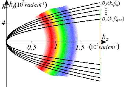
Figure 42: An example of the set of supports of the angular spectrums of plane waves of a self-imaging superposition of the tilted pulses (see text).

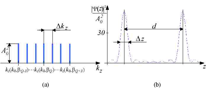
Figure 43: (a) The Fourier spectrum and (b) the spatial amplitude of a train of sinusoidal waves

The on-axis longitudinal shape of the superposition in Eq. (323) can be easily evaluated for the most practical case of a uniform superposition of $(2n+1)$ tilted pulses, centered around some carrier spatial frequency $k_{z}\left(k_{0},\beta_{Q}\right)$ (see Fig. 43). Superposition can be expressed as

$$\Psi\left(z\right)=A_{0}\frac{\sin\left[\frac{1}{2}\left(2n+1\right)\Delta k_{z}z\right]}{\sin\left(\frac{1}{2}\Delta k_{z}z\right)}\text{,}$$ (324)

where $\Delta k_{z}$ is the interval between the spatial frequencies (see Ref. o28 for example). For this case the self-imaging distance is $d=2\pi/\Delta k_{z}$ and the width of the peaks of the resulting function is $\Delta z\approx 2\pi/(2n+1)\Delta k_{z}$. The result of the evaluation of Eq. (320) for a superposition of seven tilted pulses is shown on Fig. 43b.

A numerical example of the self-imaging behavior of a superposition of five FWM’s in (323) is depicted in Fig. 41. In this example the self-imaging distance $d=2\times 10^{-5}m$, $\gamma=1$, $k_{0}=1\times 10^{7}rad{/}m$, $\sigma_{k}=3.8\times 10^{-7}m$ ($\approx 3fs$) $q=27,28,...,31$ with $\beta_{q}$ being determined by Eq. (318) ($\beta_{q}=7.6\times 10^{5}rad/m...1.3\times 10^{5}rad/m$) and $\theta_{F}\left(k_{0},\beta_{q}\right)$ by Eq. (320).

As the second example we demonstrate the self-imaging transmission of a non-trivial spatial image, depicted on Fig. 44a. The image consists of eight “pixels”– the self-imaging superpositions of FWM’s – specified in previous example. The numerical examples clearly show that the concept, in principle, is applicable for constructing wave fields that self-image three-dimensional images. Still, the experimental realization of such wave fields is not trivial.

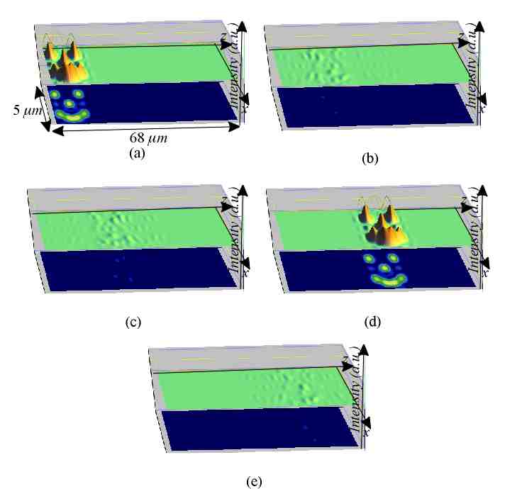
Figure 44: A numerical example of the evolution of a self-imaging spatial image (smiling human face) consisting of eight self-imaging pixels. The snapshots are taken at 19 femtosecond time intervals.

IX CONCLUSIONS

In this review we developed a physically transparent, comprehensive theory for the description of propagation-invariance of the scalar wideband wave fields in terms of Whittaker type angular spectrum of plane waves. This representation was demonstrated to be very useful in discussions on the physical nature of the localized wave transmission phenomenon and propose a general idea for optical generation of the localized waves.

X NOTATIONS USED IN THIS REVIEW

$\rho,z,\varphi$	– cylindrical coordinates system
$k_{x},k_{y},k_{z}$	– the Cartesian components of the wave vector $\mathbf{k}$
$k_{0}$	– carrier wave number
$k,\theta,\phi$	– spherical coordinates in $k$-space;
$\chi=k_{\rho}=k\sin\theta$
$\gamma$, $\gamma_{\rho}$	– see Eq. (32), (53)
$\beta,\xi$	– see Eqs. (33) and (36)
$\mu=z+ct$
$\zeta=z-ct$
$v^{g}$, $v^{p}$	– group velocity (32) and phase velocity
$a_{1},a_{2},\kappa,b,p,q$	– parameters, see Eqs. (115), (118), (155)
$\theta_{F}\left(k\right)\equiv\theta_{F}\left(k,\beta\right)$, $\theta_{F}^{\left(\rho\right)}\left(k\right)$	– see Eqs. (34), (55)
$\theta_{G}\left(k\right)$	– see Eq. (242)
$k_{F}\left(\theta\right)$	– see Eq. (35)
$\tilde{\alpha}=\frac{1}{2}\left(\frac{\omega}{c}+k_{z}\right)$
$\tilde{\beta}=\frac{1}{2}\left(\frac{\omega}{c}-k_{z}\right)$
$\tau=t_{2}-t_{1}$, $\Delta z$	– the time- and $z$ coordinate difference
$\tau_{s}$, $\sigma_{k}$, $\sigma_{z}$, $\sigma_{\rho}$	– see Eqs. (65), (66a), (66b)
$\Delta t$, $z_{\Delta}$, $z_{m}$	– see Eqs. (272), (282), (281)

$\psi\left(\mathbf{k},\omega\right)=\mathcal{F}\left[\Psi\left(\mathbf{r},t\right)\right]$	– see Eq. (9)
$A\left(k_{x},k_{y,}k_{z}\right)$	– see Eq. (13)
$A_{n}\left(k,\theta\right)$	– see Eq. (17)
$A_{z}\left(k_{x},k_{y}\right)$, $A_{xy}\left(k_{z}\right)$	– see Eq. (59), (63)
$A_{n}^{we}\left(k,\chi\right)$	– see Eqs. (21)
$B_{n}\left(k\right)$, $B_{0}\left(k\right)\equiv B\left(k\right)$	– see Eq. (40)
$\tilde{A}\left(k_{x},k_{y,}k_{z}\right)$, $\tilde{A}_{n}\left(k,\theta\right)$, $\tilde{B}_{n}\left(k\right)$	– see note after Eq. (85)
$C_{n}\left(\tilde{\alpha},\tilde{\beta},\chi\right)$	– see Eq. (22)
$\Xi\left(\chi,\beta\right)$	– see Eq. (111)
$a(k,\theta,\phi)$	– stochastic angular spectrum of plane waves

$\Psi^{\prime}\left(x,y,z,t\right)$, $\Psi\left(\rho,z,\varphi,t\right)$	– see Eqs. (10), (19)
$\mathbf{E}\left(\mathbf{r},t\right)$, $\mathbf{H}\left(\mathbf{r},t\right)$,$\mathbf{A}\left(\mathbf{r},t\right)$, $\mathbf{\Pi}^{\left(e\right)}$, $\mathbf{\Pi}^{\left(m\right)}$	– see Sec. II.1
$\Psi_{F}\left(\rho,z,\varphi,t\right)$, $\Psi_{f}\left(\rho,z,\varphi,t\right)$	– see Eqs. (42), (113)
$T\left(x,y,z,t;\phi\right)$, $F\left(x,z,t\right)$	– see Eqs. (88), (90)
$\Gamma\left(\mathbf{r}_{1},\mathbf{r}_{2},t_{1},t_{2}\right)$	– mutual coherence function, Eq. (177)
$W\left(\mathbf{r}_{1},\mathbf{r}_{2},k\right)$	– cross-spectral density
$\mathcal{A}\left(k_{1},k_{2},\theta_{1},\theta_{2},\phi_{1},\phi_{2},\right)$	– see Eq. (190), angular correlation function
$\mathcal{C}\left(k_{1},k_{2},\phi_{1},\phi_{2}\right)$	– see Eq. (199)
$\mathcal{V}\left(k,\phi\right)$	– see Eq. (199)
$\emph{s}\left(k\right)$	– see Eq. (64), frequency spectrum of light source
$\mathcal{S}\left(k\right)=\left|\emph{s}\left(k\right)\right|^{2}$	– spectral density (power spectrum) of light source

References

- (1) J. N. Brittingham, J. Appl. Phys. 54 (1983) 1179.
- (2) T. T. Wu and R. W. P. King, J. Appl. Phys. 56 (1984) 2587.
- (3) A. Sezginer, J. Appl. Phys. 57 (1984) 678.
- (4) T. T. Wu, and H. Lehmann, Appl. Phys. 58 (1985) 2064.
- (5) P. A. Bélanger, J. Opt. Soc. Am. A 1 (1984) 723.
- (6) R. W. Ziolkowski, J. Math. Phys. 26 (1985) 861.
- (7) P. A. Bélanger, J. Opt. Soc. Am. A 3 (1986) 541.
- (8) P. Hillion, J. Appl. Phys. 60 (1986) 2981.
- (9) E. Heyman, and L. P. Felsen, IEEE Trans. Antennas Propag. AP-34 (1986) 1062.
- (10) E. Heyman, and B. Z. Steinberg, J. Opt. Soc. Am. A 4 (1987) 473.
- (11) P. D. Einziger, and S. Raz, J. Opt. Soc Am. A 4 (1987) 3.
- (12) E. Heyman, B. Z. Steinberg, and L. B. Felsen, J. Opt. Soc Am. A 4 (1987) 2081.
- (13) E. Heyman, IEEE Trans. Antennas Propag. AP-37 (1989) 1604.
- (14) I. M. Besieris, A. M. Shaarawi, and R. W. Ziolkowski, J. Math. Phys. 30 (1989) 1254.
- (15) R. Donnelly, and R. Ziolkowski, Proc. R. Soc. Lond. A 440 (1993) 541.
- (16) R. Donnelly, and R. Ziolkowski, Proc. R. Soc. Lond. A 437 (1992) 673.
- (17) M. R. Palmer, and R. Donnelly, J. Math. Phys. 34 (1993) 4007.
- (18) A. M. Shaarawi, R. W. Ziolkowski, and I. M. Besieris, J. Math. Phys. 36 (1995) 5565.
- (19) P. Hillion, J. Opt. Soc. Am. A 8 (1991) 695.
- (20) A. M. Shaarawi, I. M. Besieris, and R. W. Ziolkowski, Opt. Comm. 116 (1995) 183.
- (21) P. Hillion, J. Opt. Soc. Am. A 16 (1999) 205.
- (22) P. Hillion, J. Math. Phys. 28 (1987) 1743.
- (23) M. K. Tippett, and R. W. Ziolkowski, J. Math. Phys. 32 (1991) 488.
- (24) A. M. Vengerskas, I. M. Besieris, A. M. Shaarawi, and R. W. Ziolkowski, Phys. Rev. E. 9 (1992) 937.
- (25) P. L. Overfelt, Phys. Rev. E. 52 (1995) 4387.
- (26) T. T. Wu, J. Appl. Phys. 57 (1985) 2370.
- (27) T. T. Wu, R. W. P. King, and H. -M. Shen, J. Appl. Phys. 62 (1987) 4036.
- (28) H.-M. Lee, Radio Sci. 22 (1987).
- (29) H. E. Moses and R. T. Prosser, IEEE Trans. Antennas Propag. AP-34 (1986) 188.
- (30) H. E. Moses, J. Math. Phys. 25 (1984) 1905.
- (31) R. W. Ziolkowski, Phys. Rev. A 39 (1989) 2005.
- (32) P. L. Overfelt, Phys. Rev. E. 47 (1993) 4430.
- (33) P. L. Overfelt, Phys. Rev. A 44 (1991) 3941.
- (34) P. L. Overfelt, J. Opt. Soc. Am. A 18 (2001) 1905.
- (35) I. Besieris, M. Abdel-Rahman, A. Shaarawi, and A. Chatzipetros, Progr. In Electromagn. Research 19 (1998) 1.
- (36) J. A. Campbell, and S. Soloway, J. Acoust. Soc. Am. 88 (1990) 2467.
- (37) A. N. Norris, B. S. White, and J. R. Scrieffer, Proc. Roy. Soc. London A 412 (1987) 93.
- (38) A. M. Vengsarkar, I. M. Besieris, A. M. Shaarawi, and R. W. Ziolkowski, J. Opt. Soc. Am. A 9 (1992) 937.
- (39) A. M. Shaarawi, I. M. Besieris, and R. W. Ziolkowski, J. Appl. Phys. 65 (1989) 805.
- (40) R. W. Ziolkowski, and D. K. Lewis, J. Appl. Phys. 68 (1990) 6083.
- (41) R. W. Ziolkowski, D. K. Lewis, and B. D. Cook, Phys. Rev. Lett. 62 (1989) 147.
- (42) R. W. Ziolkowski, Phys. Rev. A 44 (1991) 3960.
- (43) R. W. Ziolkowski, IEEE Trans. Antennas. Propagat. 40 (1992) 888.
- (44) R. W. Ziolkowski, I. M. Besieris, and A. M. Shaarawi, J. Opt. Soc. Am. A 10 (1993) 75.
- (45) A. M. Shaarawi, I. M. Besieris, R. W. Ziolkowski, and S. M. Sedky, J. Opt. Soc. Am. A 12 (1995) 1954.
- (46) A. M. Shaarawi, S. M. Sedky, R. W. Ziolkowski, and F. M. M. Taiel, J. Opt. Soc. Am. A 13 (1996) 1712.
- (47) S. M. Sedky, A. M. Shaarawi, I. M. Besieris, and F. M. M. Taiel, J. Opt. Soc. Am. A 13 (1996) 1719.
- (48) A. M. Shaarawi, S. M. Sedky, F. M. M. Taiel, R. W. Ziolkowski, and I. M. Besieris, J. Opt. Soc. Am. A 13 (1996) 1827.
- (49) A. M. Shaarawi, J. Opt. Soc. Am. A 14 (1997) 1804.
- (50) P. L. Overfelt, J. Opt. Soc. Am. A 14 (1997) 1087.
- (51) P. L. Overfelt, J. Opt. Soc. Am. A 16 (1999) 2239.
- (52) P. Saari and K. Reivelt, Phys. Rev. Lett. 79 (1997) 4135.
- (53) K. Reivelt and P. Saari, J. Opt. Soc. Am. A 17 (2000) 1785.
- (54) K. Reivelt and P. Saari, Phys. Rev. E 65 (2002) 046622.
- (55) K. Reivelt, Opt. Express 10 (2002) 360.
- (56) K. Reivelt and P. Saari, Phys. Rev. E 66 (2002) 056611.
- (57) J. Durnin, J. Opt. Soc. Am. A 4 (1987) 651.
- (58) J. Durnin, J. J. Miceli, Jr., and J. H. Eberly, Phys. Rev. Lett. 58 (1987) 1499.
- (59) D. DeBeer, S. R. Hartmann, and R. Friedberg, Phys. Rev. Lett. 59 (1987) 2611.
- (60) K. B. Wolf, Phys. Rev. Lett. 60 (1988) 757.
- (61) J. Durnin, J. J. Miceli Jr., and J. H. Eberly, Opt. Lett. 13 (1988) 79.
- (62) J. K. Jabczyńsky, Opt. Comm. 77 (1990) 292.
- (63) J. -Y. Lu, and J. F. Greenleaf, Ultrasound in Mol. & Biol. 17 (1991) 265.
- (64) Z. Bouchal, J. Mod. Opt. 40 (1993) 1325.
- (65) Z. L. Horváth, et al J. Opt. Soc. Am. A 14 (1997) 3009.
- (66) J.-Y. Lu, IEEE Trans. Ultrasonic. Ferroelec., Freq. Contr. 42 (1995) 1050.
- (67) S. Chávez-Cerda, G. S. McDonald, and G. H. C. New, Opt. Comm. 123 (1996) 225.
- (68) V. Kettunen, and J. Turunen, Opt. Lett. 23 (1998) 1247.
- (69) S. Chávez-Cerda, M. A. Meneses-Nava, and J. M. Hickmann, Opt. Lett. 23 (1998) 1871.
- (70) J. Turunen, A. Vasara, and A. T. Friberg, Appl. Opt. 27 (1988) 3959.
- (71) F. Gori, G. Guattari, and C. Padovani, Opt. Comm. 64 (1987) 491.
- (72) A. Vasara, J. Turunen, and A. T. Friberg, J. Opt. Soc. Am. A 6 (1989) 1748 .
- (73) S. De Nicola, Opt. Comm. 80 (1991) 299.
- (74) R. M. Hermann, and T. A Wiggins, J. Opt. Soc. Am. A 8 (1991) 932.
- (75) P. L. Overfelt, and C. S. Kennedy, J. Opt. Soc. Am. A 8 (1991) 723.
- (76) A. J. Cox, and J. D’Anna, Opt. Lett. 17 (1992) 232.
- (77) R. M. Herman, and T. A. Wiggins, Appl. Opt. 31 (1992) 5913.
- (78) J. Sochacki, Z. Jaroszewicz, L. R. Staronski, and A Kolodziejczyk, J. Opt. Soc. Am. A 10, (1993) 1765.
- (79) J. Rosen, Opt. Lett. 19 (1994) 369.
- (80) R. H. Jordan, and D. G. Hall, Opt. Lett. 19 (1994) 427.
- (81) S. Ruschin, J. Opt. Soc. Am. A 11 (1994) 3224.
- (82) J. Rosen, B. Salik, A. Yariv, and H.-K. Liu, Opt. Lett. 20 (1995) 423.
- (83) B. Salik, J. Rosen, and A. Yariv, Opt. Lett. 20 (1995) 1743.
- (84) J. Rosen, B. Salik, and A. Yariv, J. Opt. Soc. Am. A 12 (1995) 2446.
- (85) Z. Jaroszewicz, J. F. Román Dopazo, and C. Gomez-Reino, Appl. Opt. 35 (1996) 1025.
- (86) A. T. Friberg, J. Opt. Soc. Am. A 12 (1996) 743.
- (87) R. P. McDonald, S. A. Boothroyd, T. Okamoto, J. Chrostowski, and B. A. Syrett, Opt. Comm. 122 (1996) 169.
- (88) P. L. Greene, and D. G. Hall, J. Opt. Soc. Am. A 13, (1996) 962.
- (89) R. Borghi, M. Santarsiero, and F. Gori, J. Opt. Soc. Am. A 14 (1997) 23.
- (90) R. Borghi, and M. Santarsiero, Opt. Lett. 22 (1997) 262.
- (91) Z. L. Horváth et al, J. Opt. Soc. Am. A 11 (1997) 3009.
- (92) L. Niggl, T. Lanzl, and M. Maier, J. Opt. Soc. Am. A 14 (1997) 27.
- (93) Z. Jiang, J. Opt. Soc. Am. A 14 (1997) 1478.
- (94) R. Liu, B.-Z. Dong, and B.-Y. Gu, Appl. Opt. 37 (1998) 8219.
- (95) Z. Bin, and L. Zhu, Appl. Opt. 37 (1998) 2563.
- (96) W.-X. Cong, N.-X. Chen, and B.-Y. Gu, J. Opt. Soc. Am. A 15 (1998) 2362.
- (97) R. Piestun, Y. Y. Schechner, and J. Shamir, J. Opt. Soc. Am. A 17 (2000) 294.
- (98) J. H. McLeod, J. Opt. Soc. Am. 44 (1954) 592.
- (99) H. S. Lee, B. W. Stewart, D. Will, and H. Fenichel, Appl. Phys. Lett. 59 (1991) 3096.
- (100) A. J. Cox, and D. C. Dibble, Appl. Opt. 30 (1991) 1330.
- (101) Y. Lin, W. Seka, J. H. Eberly, H. Huang, and L. Brown, Appl. Opt. 31 (1992) 2708.
- (102) R. P. MacDonald, J. Chrostowski, S. A. Boothroyd, and B. A. Syrett, Appl. Opt. 32 (1993) 6470.
- (103) V. P. Koronkevich, I. A. Mikhaltsova, E. G. Churin, and Y. I. Yurlov, Appl. Opt. 34 (1995) 5761.
- (104) J. -Y. Lu, and J. G. Greenleaf, IEEE Trans. Ultrason. Ferroelec., Freq. Contr. 39 (1992) 19.
- (105) J. Fagerholm, A. T. Friberg, J. Huttunen, D. P. Morgan, and M. M. Salomaa, IEEE Ultrasonics Symposium, (1995) 687.
- (106) J. Fagerholm, A. T. Friberg, J. Huttunen, D. Morgan, and M. M. Salomaa, Phys. Rev. E 54 (1996) 4347.
- (107) J. -Y. Lu, and J. F. Greenleaf, Ultrasound in Mol. & Biol. 20 (1994) 403.
- (108) A. T. Friberg, J. Fagerholm, and M. M. Salomaa, Opt. Comm. 136 (1997) 207.
- (109) E. Recami, Physica A 252 (1998) 586.
- (110) J. -Y. Lu, and S. He, Opt. Comm. 161 (1999) 187.
- (111) J. Salo, J. Fagerholm, A. T. Friberg, and M. M. Salomaa, Phys. Rev. E 62 (2000) 4261.
- (112) A. M. Shaarawi, B. H. Tawfik, and I. M. Besieris, Phys. Rev. E 66 (2002) 046626.
- (113) B. Hafizi, and P. Sprangle, J. Opt. Soc. Am. A 8 (1991) 705.
- (114) D. Mugnai, A. Ranfagni, and R. R. Ruggeri, Phys. Rev. Lett. 84 (2000) 4830.
- (115) E. Capelas de Oleveira, W. A. Rodrigues Jr., D. S. Thober, and A. L. Xavier Jr., Phys. Lett. A 284 (2001) 298.
- (116) W. A. Rodrigues Jr., D. S. Thober, and A. L. Xavier Jr., Phys. Lett. A 284 (2001) 217.
- (117) D. Mugnai, Phys. Lett. A 284 (2001) 304.
- (118) T. Sauter, and F. Paschke, Physics Lett. A 285 (2001) 1.
- (119) I. Alexeev, K. Y. Kim, and H. M. Milchberg, Phys. Rev. Lett. 88 (2002) 073901.
- (120) P.Saari, In Ultrafast Processes in Spectroscopy (Eds. O.Svelto, S. De Silvestri, G. Denardo), Plenum Press, New York (1996) pp. 151-156.
- (121) P. Saari, and H. Sõnajalg, Laser Physics 7, (1997) 32.
- (122) H. Sõnajalg and P. Saari, Opt. Lett. 21 (1996) 1162.
- (123) H. Sõnajalg, M. Rätsep and P. Saari, Opt. Lett. 22 (1997) 310.
- (124) P.Saari, In Ultrafast Phenomena XI (Eds. T. Elsaesser, J. G. Fujimoto, D.A. Wiersma, W. Zinth), Springer Verlag, Berlin – Heidelberg – New York, (1998) pp. 121-123.
- (125) S. R. Mishra, Opt. Comm. 85 (1991) 159.
- (126) Z. Bouchal, and M. Olivik, J. Mod. Opt. 42 (1995) 1555.
- (127) D. G. Hall, Opt. Lett. 21 (1996) 9.
- (128) R. W. Hellwarth, and P. Nouchi, Phys. Rev. E 54 (1996) 889.
- (129) P. Vahimaa, V. Kettunen, M. Kuittinen, J. Turunen, and A. T. Friberg, J. Opt. Soc. Am. A 14 (1997) 1817.
- (130) S. Feng, H. G. Winful and R. W. Hellwarth, Opt. Lett. 23 (1998) 385.
- (131) Z. Bouchal, J. Bajer, and M. Bertolotti, J. Opt. Soc. Am. A 15 (1998) 2172.
- (132) D. You, and P. H. Bucksbaum, J. Opt. Soc. Am. B 7 (1997) 1651.
- (133) J. Courtial, Opt. Comm. 151 (1998) 1.
- (134) T. Melamed, and L. B. Felsen, J. Opt. Soc. Am. A 15 (1998) 1268.
- (135) T. Melamed, and L. B. Felsen, J. Opt. Soc. Am. A 15 (1998) 1277.
- (136) R. Simon, and N. Mukunda, J. Opt. Soc. Am. A 15 (1998) 2146.
- (137) C. J. R. Sheppard, and S. Saghafi, J. Opt. Soc. Am. A 16 (1999) 1381.
- (138) M. A. Porras, J. Opt. Soc. Am. B 16 (1999) 1468.
- (139) Q. Cao, J. Opt. Soc. Am. B 16 (1999) 1786.
- (140) S. Fend, H. G. Winful, J. Opt. Soc. Am. A 16 (1999) 2500.
- (141) M. A. Porras, R. Borghi, and M. Santarsiero, Phys. Rev. E. 62 (2000) 5729.
- (142) C. J. R. Sheppard, J. Opt. Soc. Am. A 18 (2001) 1579.
- (143) C. J. R. Sheppard, J. Opt. Soc. Am. A 18 (2001) 1.
- (144) P. Saari, Opt. Express 8 (2001) 590.
- (145) J. Opt. Soc. Am. A 18 (2001) 1588.
- (146) P. Saari, Laser Physics, 12 (2002) 219.
- (147) F. Gori, G. Guattari, and C. Padovani, Opt. Comm. 64 (1987) 311.
- (148) A. T. Friberg, A. Vasara, and J. Turunen, Phys. Rev. A 43 (1991) 7079.
- (149) J. Turunen, A. Vasara, and A. T. Friberg, J. Opt. Soc. Am. A 8 (1991) 282.
- (150) G. A. Deschamps, Electron. Lett. 7 (1971) 684.
- (151) L. P. Felsen, Symp. Math. 18 (1976) 39.
- (152) K. B. Hill, S. S. Basinger, R. A. Stack, and D. J. Brady, Appl. Opt. 36 (1997) 3948.
- (153) H. Arimoto, and Y. Ohtsuka, Opt. Lett. 22 (1997) 958.
- (154) J. Tu, and S. Tamura, J. Opt. Soc. Am. A 15 (1998) 202.
- (155) D. Mendlovic, G. Shabtay, A. W. Lohmann, and N. Konforti, Opt. Lett. 23 (1998) 1084.
- (156) A- G. Engen, S. A. Diddams, and T. S. Clement, Appl. Opt. 37 (1998) 5679.
- (157) A. W. Lohmann, D. Mendlovic, and G. Shabtay, J. Opt. Soc. Am. A 16, (1999) 359.
- (158) Z. Bin, L. Zhu, ”Diffraction property of an axicon in oblique illumination,” Appl. Opt. 37, 2563-2568 (1998).
- (159) S. Solimeno, B. Crosignani, and P. DiPorto, Guiding , Diffraction, and Confinement of Optical Radiation (Academic Press, INC., 1986).
- (160) In Optics, Opto-Mechanics, Lasers, Instruments (Melles Griot, Irvine, Calif., 1995).
- (161) C. W. McCutchen, J. Opt. Soc. Am. 54 (1964) 240.
- (162) G. Bjeitmjen, and A. Erdjeii, Tablitsõ intjegralnõh prjeobrazovanii (T.1, M. Nauka 1969).
- (163) L. Mandel, and E. Wolf, Optical coherence and quantum optics, (Cambridge University Press, 1995).
- (164) J. D. Jackson, Classical Electrodynamics (Wiley, New York, 1999).
- (165) J. A. Stratton, Electromagnetic Theory (McGraw-Hill, New York, 1941).
- (166) A. E. Siegman, Lasers, (University Science Books, Mill Valley, CA, 1986).
- (167) O. Svelto, Principles of Lasers (3rd ed. Plenum Press 1989).
- (168) W. D. Montgomery, J. Opt. Soc. Am. 57 (1967) 772.
- (169) J. Turunen, and A. T. Friberg, Pure. Appl. Opt. 2 (1992) 51.
- (170) R. Piestun, Y. Y. Schechner, and J. Shamir, Opt. Lett. 22 (1997) 200.
- (171) R. Piestun, and J. Shamir, J. Opt. Soc. Am. A 15 (1998) 3039.
- (172) J. Azaña and M. A. Muriel, Opt. Lett. 24 (1999) 1672.
- (173) Z. Bouchal, and J. Wagner, Opt. Comm. 176 (2000) 299.
- (174) J. Wagner, and Z. Bouchal, Opt. Comm. 176 (2000) 309.
- (175) Z. Bouchal, and M. Bertolotti, J. Mod. Opt. 47 (2000) 1455.
- (176) H. Wang, C. Zhou, L. Jianlang and L. Liu, Microwave and Opt. Technol. Lett. 25 (2000) 184.
- (177) J. Tervo, and J. Turunen, Opt. Express 9 (2001) 622.
- (178) J. Tervo, and J. Turunen, Opt. Express 9 (2001) 9
- (179) Z. Bouchal, and R. Horák, J. Mod. Opt. 48 (2001) 333.
- (180) Z. Bouchal, Proc. SPIE, vol. 4356 (2001) 217.
- (181) J. Salo, and M. M. Salomaa, Pure. Appl. Opt. 3 (2001) 366.
- (182) P. Pääkkönen, J. Tervo, P. Vahimaa, J. Turunen, and F. Gori, Opt. Express 10 (2002) 949.
- (183) G. C. Sherman, A. J. Devaney, and L. Mandel, Opt. Comm. 6 (1972) 115.
- (184) M. Nieto-Vesperinas, Opt. Comm. 67 (1988) 391.
- (185) E. Wolf, and J. T. Foley, Opt. Lett. 23 (1998) 16.
- (186) G. C. Sherman, J. J. Stamnes, and É. Lalor, J. Math. Phys. 17 (1976) 760.
- (187) S. Szatmári, P. Simon, and M. Feuerhake, Opt. Lett. 15 (1996) 1156.
- (188) C. W. McCutchen, J. Opt. Soc. Am. 54, (1963) 240.
- (189) G. Indebetouw, J. Opt. Soc. Am. A 6 (1989) 150.
- (190) M. Testorf, and M. Fiddy, J. Opt. Soc. Am. A 16 (1999) 1806.