A comparison of methods for confidence intervals

Abstract

Comparisons are carried out of the confidence intervals constructed with Neyman’s frequentist method and with the $\Delta L=1/2$ likelihood method, using the example of low-statistics life time estimates.

I P.d.f. for life time estimators

For a given value $\tau$ of the true life time, the P.D.F. of a measurement is

$$\frac{\,\mathrm{d}W}{\,\mathrm{d}t}=\frac{1}{\tau}\exp\left(-\frac{t}{\tau}\right),$$

and so for an experiment with $n$ measurements

$$\,\mathrm{d}W=\frac{1}{\tau^{n}}\cdot\prod\limits_{k=1}^{n}\,\mathrm{d}t_{k}\cdot\exp\left(-\frac{t_{k}}{\tau}\right).$$ (1)

The negative log likelihood function is

$$L=n\ln\tau+\frac{1}{\tau}\cdot\sum\limits_{k=1}^{n}t_{k}.$$ (2)

The maximum likelihood estimator of the lifetime can easily be found minimizing $L$

$$\hat{\tau}=\frac{1}{n}\sum\limits_{k=1}^{n}t_{k};\;\;\;\min L=L_{0}=n+n\ln\hat{\tau},$$ (3)

so the probability (1) can be transformed to

$$\frac{\,\mathrm{d}W}{\,\mathrm{d}\hat{\tau}}=\frac{1}{(n-1)!}\cdot\left(\frac{n\hat{\tau}}{\tau}\right)^{n-1}\cdot\frac{n}{\tau}\cdot\exp\left(-\frac{n\hat{\tau}}{\tau}\right).$$ (4)

Given some true value $\tau$ then for any algorithm that defines a confidence interval $\hat{\tau}^{+\Delta\tau^{(+)}}_{-\Delta\tau^{(-)}}$ we can evaluate the coverage $P$:

$$P=\frac{1}{(n-1)!}\cdot\frac{n}{\tau}\cdot\int\limits_{\hat{\tau_{1}}}^{\hat{\tau_{2}}}\left(\frac{n\hat{\tau}}{\tau}\right)^{n-1}\cdot\exp\left(-\frac{n\hat{\tau}}{\tau}\right)\,\mathrm{d}\hat{\tau},$$ (5)

where $\hat{\tau_{1}}+\Delta\tau^{(+)}=\tau;\;\;\;\hat{\tau_{2}}-\Delta\tau^{(-)}=\tau.$

II Likelihood Function confidence interval

The conventional Likelihood function method for finding a 68% confidence interval Hudson ; LF_method1 is to find the values of $\tau$ for which

$$\Delta L=L-L_{0}=\frac{1}{2}.$$

In our case

$$\Delta L=n\cdot\left(\frac{\hat{\tau}}{\tau}-1+\ln\frac{\tau}{\hat{\tau}}\right)=\frac{1}{2}.$$ (6)

For example, for $n=5$ the limits are

$$\left[\tau_{1},\tau_{2}\right]=\left[0.6595\hat{\tau},1.6212\hat{\tau}\right].$$ (7)

The coverage of this interval, from Equation (5), is

$$\frac{1}{4!}\cdot\frac{5}{\tau}\cdot\int\limits_{\hat{\tau_{1}}}^{\hat{\tau_{2}}}\left(\frac{5\hat{\tau}}{\tau}\right)^{4}\cdot\exp\left(-\frac{5\hat{\tau}}{\tau}\right)\,\mathrm{d}\hat{\tau}=0.6747,\;\;$$

where the integration limits, corresponding to (7), are

$$\left[\hat{\tau_{1}},\hat{\tau_{2}}\right]=\left[0.6168\tau,1.5163\tau\right].$$

The coverage is close to, but significally different from, the nominal value of 0.6827.

Examples of confidence intervals obtained by this means are shown in Table 1, as the values in parantheses. The 95% confidence interval was obtained using the rule $\Delta L=2$, and 90% upper limit using a one side interval for which

$$\Delta L=\left[\mbox{erf}^{-1}\left(2\cdot 0.9-1\right)\right]^{2}\approx 0.821.$$

The coverage given by such intervals is shown in Fig. 1, evaluated using a Monte Carlo method.

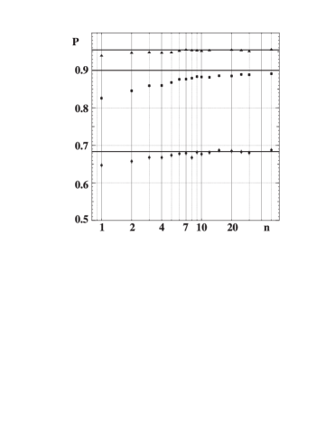
Figure 1: Coverage for likelihood function confidence intervals, evaluated by Monte Carlo. Statistical errors are shown when they exceed the size of polymarker. $\blacktriangle$ — 95% Conf.Interv., $\blacksquare$ — 90% Upper limit, $\bullet$ — 68% Conf.Interv.

III Bayesian confidence interval

For comparison we can estimate a Bayesian confidence interval for the same example of $n=5$. In the Bayesian approach Jeffreys ; BayesAll ; Neyman2 , the likelihood function is considered to be a probability density for the true parameter $\tau$. Assuming a flat prior distribution for $\tau$ this is

$$\frac{\,\mathrm{d}W}{\,\mathrm{d}\tau}=P(\tau)\sim{\cal L}=\frac{1}{\tau^{n}}\cdot\exp\left(-\frac{n\hat{\tau}}{\tau}\right).$$

After normalization (for $n\geq 2$) this becomes:

$$P(\tau)=\frac{\left(n\hat{\tau}\right)^{n-1}}{(n-2)!\cdot\tau^{n}}\cdot\exp\left(-\frac{n\hat{\tau}}{\tau}\right),$$

which for $n=5$ gives

$$\int\limits_{0}^{\tau}\,\mathrm{d}W=\left[1+\frac{5\hat{\tau}}{\tau}+\frac{1}{2}\left(\frac{5\hat{\tau}}{\tau}\right)^{2}+\frac{1}{6}\left(\frac{5\hat{\tau}}{\tau}\right)^{3}\right]\cdot e^{-\frac{5\hat{\tau}}{\tau}}.$$ (8)

The 68% central confidence region for this distribution is (see Fig. 2):

Figure 2: Probability density function for the true value of the parameter $\tau$ in a Bayesian approach (Equation (8) with $n=5$ and $\hat{\tau}=1$). The shaded regions are the 16% “tails”.

$$\tau=\hat{\tau}\cdot\left(1^{+1.3974}_{-0.1552}\right)\;\;$$

The coverage of this region is actually not 68.27% but 64.31%.

IV Neyman’s confidence interval

Neyman Neyman1 ; Neyman2 ; Barlow proposed a frequentist construction of a confidence zone (or confidence belt) as follows (see Figure 3):

1. One obtains functions $\hat{\tau}_{1}(\tau)$ and $\hat{\tau}_{2}(\tau)$ of the true parameter $\tau$ such that

   $$\begin{array}[]{l}\int\limits_{0}^{\hat{\tau}_{1}(\tau)}\frac{\,\mathrm{d}W(\hat{\tau};\tau)}{\,\mathrm{d}\hat{\tau}}\,\mathrm{d}\hat{\tau}=\frac{1-\beta}{2};\\[11.38109pt] \int\limits_{\hat{\tau}_{2}(\tau)}^{\infty}\frac{\,\mathrm{d}W(\hat{\tau};\tau)}{\,\mathrm{d}\hat{\tau}}\,\mathrm{d}\hat{\tau}=\frac{1-\beta}{2},\end{array}$$

   where $\beta$ is the confidence level required, here $\beta=0.6827$. For $n=5$ these are simply $\hat{\tau}_{1}(\tau)=0.568\tau$, $\hat{\tau}_{2}(\tau)=1.433\tau$, as shown in Figure 3.

2. One defines the inverse functions

   $$\tau_{1}(\hat{\tau})=\hat{\tau}_{2}^{-1}(\hat{\tau});\;\;\;\tau_{2}(\hat{\tau})=\hat{\tau}_{1}^{-1}(\hat{\tau})$$

   which, for a given value of $\hat{\tau}$, define the borders of the confidence interval for $\tau$, with coverage $\beta$.

   In our example, there are $\tau_{1}(\hat{\tau})=0.698\hat{\tau}$, $\tau_{2}(\hat{\tau})=1.760\hat{\tau}$.

   Thus the result of a lifetime experiment of this type can be written

   $$\tau=\hat{\tau}\cdot\left(1^{+0.760}_{-0.302}\right).$$

   The coverage evaluated is 0.6826 — the difference of 0.0001 is purely due to rounding errors.

Table 1 shows these intervals for several values of $n$, with the likelihood approximation shown in parantheses for comparison.

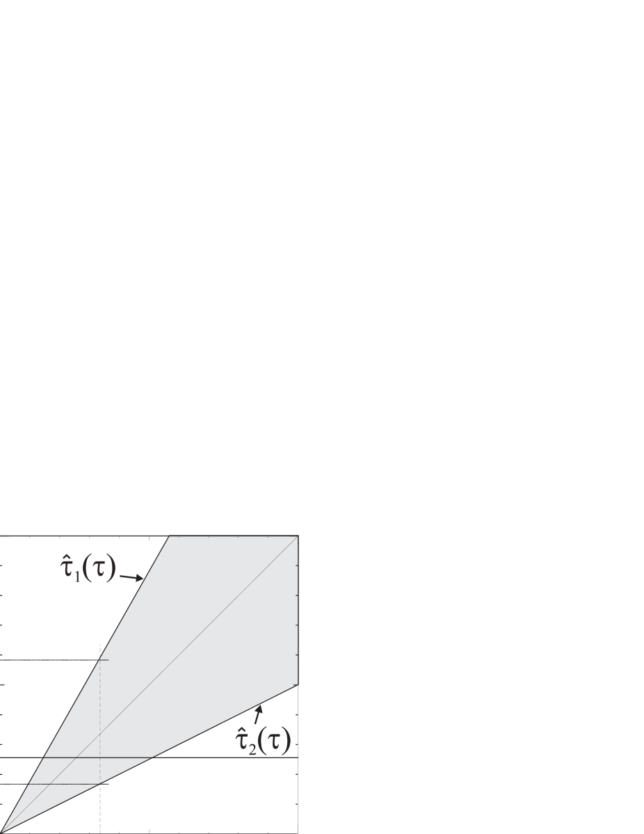
Figure 3: Illustration of the construction of a confidence zone (or confidence belt).

Table 2 compares the coverage of all three methods for the $n=5$ case.

Table 1: Lifetime confidence intervals obtained by Neyman’s method for various values of $n$, the number of measurements, and confidence levels.

$n$	68% C.L.		95% C.L.		90% C.L.
	$\frac{\Delta\tau^{(-)}}{\hat{\tau}}$	$\frac{\Delta\tau^{(+)}}{\hat{\tau}}$	$\frac{\Delta\tau^{(-)}}{\hat{\tau}}$	$\frac{\Delta\tau^{(+)}}{\hat{\tau}}$	upper limit
1	0.457 (0.576)	4.789 (2.314)	0.736 (0.778)	42.45 (18.06)	$9.49\hat{\tau}$ ($8.49\hat{\tau}$)
2	0.394 (0.469)	1.824 (1.228)	0.648 (0.682)	7.690 (5.305)	$3.76\hat{\tau}$ ($2.76\hat{\tau}$)
3	0.353 (0.410)	1.194 (0.894)	0.592 (0.621)	4.031 (3.164)
4	0.324 (0.370)	0.918 (0.725)	0.551 (0.576)	2.781 (2.314)
5	0.302 (0.341)	0.760 (0.621)	0.519 (0.541)	2.159 (1.858)
6	0.284 (0.318)	0.657 (0.550)	0.492 (0.513)	1.786 (1.571)
7	0.270 (0.299)	0.584 (0.497)	0.470 (0.489)	1.538 (1.374)
8	0.257 (0.284)	0.529 (0.456)	0.452 (0.469)	1.359 (1.228)
9	0.247 (0.271)	0.486 (0.423)	0.435 (0.451)	1.225 (1.116)
10	0.237 (0.260)	0.451 (0.396)	0.421 (0.436)	1.119 (1.027)
20	0.182 (0.194)	0.285 (0.261)	0.331 (0.341)	0.654 (0.621)
50	0.124 (0.129)	0.164 (0.156)	0.232 (0.237)	0.356 (0.346)

Table 2: Coverage of all three methods for $n=5$

Method	Negative error	Positive error	Coverage, %
	${\Delta\tau^{(-)}}/{\hat{\tau}}$	${\Delta\tau^{(+)}}/{\hat{\tau}}$
Likelihood	0.341	0.621	67.47
Bayesian	0.155	1.397	64.31
Neyman’s	0.302	0.760	68.26

V Conclusion

• Neyman’s method for confidence intervals provides exact coverage, by construction.

• The intervals from $\Delta L=1/2$ agree well with the Neyman intervals for large $n$, but differ for small $n$, as can be seen in Table 1. In such cases they undercover, i.e. the interval is smaller than the true one.

• Bayesian confidence intervals give very different results, and can undercover or overcover.

References

• (1) Derek J. Hudson. Lectures on elementary statistics and probability, CERN, Geneva, 1963
• (2) A.G.Frodesen, O.Skjeggestad, H.Toffe. “Probability and statistics in particle physics”. Universitetsforlaget, Oslo, 1979
• (3) H.Jeffreys. “Theory of probability”,2nd edn, Oxford Univ. Press, 1948.
• (4) B.P.Carlin and T.A.Louis. “Bayes and empirical Bayes methods for data analysis”, Chapman & Hall, London, 1996
• (5) M.Kendall and A.Stuart. “The advanced theory of statistics”, vol. 2, “Inference and relationship”. Macmillan Publishing Co., New York, 1978.
• (6) J.Neyman. “Outline of a theory of statistical estimation based on the classical theory of probability”. Phil. Trans. A, 236 (1937) 333.
• (7) R.J.Barlow. “Statistics. A guide to the use of statistical methods in the physical sciences.” John Wiley & Sons ltd., Chichester, England, 1989