Lagrangian turbulence in the Adriatic Sea as computed from drifter data: effects of inhomogeneity and nonstationarity

Abstract

The properties of mesoscale Lagrangian turbulence in the Adriatic Sea are studied from a drifter data set spanning 1990-1999, focusing on the role of inhomogeneity and nonstationarity. A preliminary study is performed on the dependence of the turbulent velocity statistics on bin averaging, and a preferential bin scale of $0.25^{{}^{\circ}}$ is chosen. Comparison with independent estimates obtained using an optimized spline technique confirms this choice. Three main regions are identified where the velocity statistics are approximately homogeneous: the two boundary currents, West (East) Adriatic Current, WAC (EAC), and the southern central gyre, CG. The CG region is found to be characterized by symmetric probability density function of velocity, approximately exponential autocorrelations and well defined integral quantities such as diffusivity and time scale. The boundary regions, instead, are significantly asymmetric with skewness indicating preferential events in the direction of the mean flow. The autocorrelation in the along mean flow direction is characterized by two time scales, with a secondary exponential with slow decay time of $\approx$ 11-12 days particularly evident in the EAC region. Seasonal partitioning of the data shows that this secondary scale is especially prominent in the summer-fall season. Possible physical explanations for the secondary scale are discussed in terms of low frequency fluctuations of forcings and in terms of mean flow curvature inducing fluctuations in the particle trajectories. Consequences of the results for transport modelling in the Adriatic Sea are discussed.

1 Introduction

The Adriatic Sea is a semienclosed sub-basin of the Mediterranean Sea (Fig.1a). It is located in a central geo-political area and it plays an important role in the maritime commerce. Its circulation has been studied starting from the first half of the nineteen century (Poulain and Cushman-Roisin,, 2001), so that its qualitative characteristics have been known for a long time. A more quantitative knowledge of the oceanography of the Adriatic Sea, on the other hand, is much more recent, and due to the systematic studies of the last decades using both Eulerian and Lagrangian instruments (Poulain and Cushman-Roisin,, 2001). In particular, a significant contribution to the knowledge of the surface circulation has been provided by a drifter data set spanning 1990-1999, recently analyzed by Poulain, (2001). These data provide a significant spatial and temporal coverage, allowing to determine the properties of the circulation and of its variability.

In Poulain, (2001), the surface drifter data set 1990-1999 has been analyzed to study the general circulation and its seasonal variability. The results confirmed the global cyclonic circulation in the Adriatic Sea seen in earlier studies (Artegiani et al.,, 1997), with closed recirculation cells in the central and southern regions. Spatial inhomogeneity is found to be significant not only in the mean flow but also in the Eddy Kinetic Energy (EKE) pattern, reaching the highest values along the coast in the southern and central areas, in correspondence to the strong boundary currents. The analysis also highlights the presence of a marked seasonal signal, with the coastal currents being more developed in summer and fall, and the southern recirculating cell being more pronounced in winter.

In addition to the information on Eulerian quantities such as mean flow and EKE, drifter data provide also direct information on Lagrangian properties such as eddy diffusivity $K$ and Lagrangian time scales $T$, characterizing the turbulent transport of passive tracers in the basin. The knowledge of transport and dispersion processes of passive tracers is of primary importance in order to correctly manage the maritime activities and the coastal development of the area, especially considering that the Adriatic is a highly populated basin, with many different antropic activities such as agriculture, tourism, industry, fishing and military navigation.

In Poulain, (2001), estimates of $K$ and $T$ have been computed providing values of $K\approx 2\times 10^{7}\,\mathrm{cm^{2}~{}sec^{-1}}$ and $T\approx 2\,\mathrm{days}$, averaged over the whole basin and over all seasons. Similar results have been obtained in a previous paper (Falco et al.,, 2000), using a restricted data set spanning 1994-1996. In Falco et al., (2000), the estimated values have also been used as input parameters for a simple stochastic transport model, and the results have been compared with data, considering patterns of turbulent transport and dispersion from isolated sources. The comparison in Falco et al., (2000) is overall satisfactory, even though some differences between data and model persist, especially concerning first arrival times of tracer particles at given locations. These differences might be due to various reasons. One possibility is that the use of global parameters in the model is not appropriate, since it does not take into account the statistical inhomogeneity and nonstationarity of the parameter values. Alternatively, the differences might be due to some inherent properties of turbulent processes, such as non-gaussianity or presence of multiple scales in the turbulent field, which are not accounted for in the simple stochastic model used by Falco et al., (2000). These aspects are still unclear and will be addressed in the present study.

In this paper, we consider the complete data set for the period 1990-1999 as in Poulain, (2001), and we analyze the Lagrangian turbulent component of the flow, with the goal of

— identifying the main statistical properties;

— determining the role of inhomogeneity and nonstationarity.

The results will provide indications on suitable transport models for the area.

Inhomogeneity and nonstationarity for standard Eulerian quantities such as mean flow and EKE have been fully explored in Poulain, (2001), while only preliminary results have been given for the Lagrangian statistics. Furthermore, the inhomogeneity of probability density function (pdf) shapes (form factors like skewness and kurtosis) have not been analyzed yet. In this paper, the spatial dependence of Lagrangian statistics is studied first, dividing the Adriatic Sea in approximately homogeneous regions. An attempt is then made to consider the effects on non-stationarity, grouping the data in seasons, similarly to what done in Poulain, (2001) for the Eulerian statistics.

The paper is organized as follows. A brief overview of the Adriatic Sea and of previous results on its turbulent properties are provided in Section 2. In Section 3, information on the drifter data set and on the methodology used to compute the turbulent statistics are given. The results of the analysis are presented in Section 4, while a summary and a discussion of the results are provided in Section 5.

2 Background

2.1 The Adriatic Sea

The Adriatic Sea is the northernmost semi-enclosed basin of the Mediterranean connected to the Ionian Sea at its southern end through the Strait of Otranto (Fig. 1). The Adriatic basin, which is elongated and somewhat rectangular (800 km by 200 km), can be divided into three distinct regions generally known as the northern, middle and southern Adriatic (Cushman-Roisin et al.,, 2001). The northern Adriatic lies on the continental shelf, which slopes gently southwards to a depth of about 100 m. The middle Adriatic begins where the bottom abruptly drops from 100 m to over 250 m to form the Mid-Adriatic Pit (also called Jabuka Pit) and ends at the Palagruza Sill, where the bottom rises again to approximately 150 m. Finally, the southern Adriatic, extending from Palagruza Sill to the Strait of Otranto (780 m deep) is characterized by an abyssal basin called the South Adriatic Pit, with a maximum depth exceeding 1200 m. The western coast describes gentle curves, whereas the eastern coast is characterized by numerous channels and islands of complex topography (Fig. 1a).

The winds and freshwater runoff are important forcings of the Adriatic Sea. The energetic northeasterly bora and the southeasterly sirocco winds are episodic events that disrupt the weaker but longer-lasting winds, which exist the rest of the time (Poulain and Raicich,, 2001); the Po River in the northern basin provides the largest single contribution to the freshwater runoff, but there are other rivers and land runoff with significant discharges (Raicich,, 1996). Besides seasonal variations, these forcings are characterized by intense variability on time scales ranging between a day and a week.

The Adriatic Sea mean surface flow is globally cyclonic (Fig. 1b) due to its mixed positive-negative estuarine circulation forced by buoyancy input from the rivers (mainly the Po River) and by strong air-sea fluxes resulting in loss of buoyancy and dense water formation. The Eastern Adriatic Current (EAC) flows along the eastern side from the eastern Strait of Otranto to as far north as the Istrian Peninsula. A return flow (the WAC) is seen flowing to the southeast along the western coast (Poulain,, 1999, 2001). Re-circulation cells embedded in the global cyclonic pattern are found in the lower northern, the middle and the southern sub-basins, the latter two being controlled by the topography of the Mid and South Adriatic Pits, respectively. These main circulation patterns are constantly perturbed by higher-frequency currents variations at inertial/tidal and meso- (e.g., 10-day time scale; Cerovecki et al.,, 1991) scales. In particular, the wind stress is an important driving mechanism, causing transients currents that can be an order of magnitude larger than the mean circulation. The corresponding length scale is 10-20 km, i.e., several times the baroclinic radius of deformation, which in the Adriatic can be as short as 5 km (Cushman-Roisin et al.,, 2001).

2.2 Turbulent transport in the Adriatic Sea and previous drifter studies

Drifter data are especially suited for transport studies since they move in good approximation following the motion of water parcels (Niiler et al.,, 1995). As such, drifter data have often been used in the literature to compute parameters to be used in turbulent transport and dispersion models (Davis,, 1991, 1994). In the Adriatic Sea, as mentioned in the Introduction, turbulent parameters have been previously computed by Falco et al., (2000) and Poulain, (2001) as global averages over the basin. A brief overview is given in the following.

2.2.1 Models of turbulent transport and parameter definitions

The transport of passive tracers in the marine environment is usually regarded as due to advection of the “mean” flow, i.e., of the large scale component of the flow $\mathbf{u}(\mathbf{x},t)$, and to dispersion caused by the “turbulent” flow, i.e., of the mesoscale and smaller scale flow. The simplest possible model used to describe these processes is the advection-diffusion equation,

$$\partial C/\partial t+\nabla\cdot(\mathbf{U}C)=\nabla\cdot(\mathbf{K}\nabla C)$$ (1)

where $C$ is the average concentration of a passive tracer, $\mathbf{U}$ is the mean flow field and $\mathbf{K}$ is the diffusivity tensor defined as:

$$K_{ij}=\int_{o}^{\infty}R_{ij}(\tau)d\tau$$ (2)

where $\mathbf{R}(\tau)$ is the Lagrangian autocovariance,

$$R_{ij}(\tau)=\langle u_{i}^{\prime}(t)u_{j}^{\prime}(t+\tau)\rangle$$ (3)

with $\langle\cdot\rangle$ being the ensemble average and $\mathbf{u}^{\prime}=\mathbf{u}-\mathbf{U}$ being the turbulent Lagrangian velocity, i.e., the residual velocity following a particle. Note that in this definition, $\mathbf{R}$ depends only on the time lag $\tau$, consistently with an homogeneous and steady situation. In fact, non homogeneous and unsteady flows do not allow for a consistent definition of the above quantities.

The advection-diffusion equation Eq. (1) can be correctly applied only in presence of a clear scale separation between the scale of diffusion mechanism and the scale of variation of the quantity being transported (Corrsin,, 1974). Generalizations of Eq. (1) are possible, for example introducing a “history term” in Eq. (1) that takes into account the interactions between $\mathbf{U}$ and $\mathbf{u}^{\prime}$ (e.g.,  Davis,, 1987). Alternatively, a different class of models can be used, that are easily generalizable and are based on stochastic ordinary differential equation describing the motion of single tracer particles (e.g.,  Griffa,, 1996; Berloff and McWilliams,, 2002).

A general formulation was given by Thomson, (1987) and further widely used. The stochastic equations describing the particle state $\mathbf{z}$ are

$$\,\mathrm{d}z_{i}=a_{i}\,\mathrm{d}t+b_{ij}\,\mathrm{d}W_{j}$$ (4)

where $\,\mathrm{d}\mathbf{W}$ is a random increment from a normal distribution with zero mean and second order moment $\langle\,\mathrm{d}W_{i}(t)\,\mathrm{d}W_{j}(s)\rangle=\delta_{ij}\delta(t-s)\,\mathrm{d}t$.

Equation (1) can be seen as equivalent to the simplest of these stochastic models, i.e., the pure random walk model, where the particle state is described by the positions, i.e., $\mathbf{z}\equiv\mathbf{x}$ only, which are assumed to be Markovian while the velocity $\mathbf{u}^{\prime}$ is a random process with no memory (zero-order model). A more general model can be obtained considering the particle state defined by its position and velocity. Thus $\mathbf{z}\equiv(\mathbf{x},\mathbf{u}^{\prime})$ are joint Markovian, so that the turbulent velocity $\mathbf{u}^{\prime}$ has a finite memory scale, $\mathbf{T}$ (first-order model). In this case the model can also be applied for times shorter than the characteristic memory time $T$, in contrast to the zeroth-order model. If times for which acceleration is significantly correlated is important, second order models should be used (Sawford,, 1999). Higher order models are possible (see, e.g.,  Berloff and McWilliams,, 2002) but they require some knowledge on the supposed universal behavior of very elusive quantities such as time derivatives of tracer acceleration.

For a homogeneous and stationary flow with independent velocity components, the first-order model can be written for the fluctuating part $\mathbf{u}^{\prime}$ for each component and corresponds to the linear Langevin equation (i.e., the Ornstein-Uhlenbeck process, see, e.g., Risken,, 1989):

$$\,\mathrm{d}x_{i}=(U_{i}+u_{i}^{\prime})\,\mathrm{d}t$$ (5)

$$\,\mathrm{d}u_{i}^{\prime}=-\frac{u_{i}^{\prime}}{T_{i}}\,\mathrm{d}t+\sqrt{\frac{2\sigma_{i}^{2}}{T_{i}}}\,\mathrm{d}W_{i}$$ (6)

where $\sigma_{i}^{2}$ and $T_{i}$ are the variance and the correlation time scale of $u_{i}^{\prime}$, respectively.

For the model (5–6), $u_{i}^{\prime}$ is Gaussian and

$$R_{ii}(\tau)=\sigma_{i}^{2}\exp{(-\frac{\tau}{T_{i}})},$$ (7)

so that $T_{i}$

$$T_{i}=\frac{1}{\sigma_{i}^{2}}\int_{o}^{\infty}R_{ii}(\tau)=\frac{K_{ii}}{\sigma_{i}^{2}}$$ (8)

corresponds to the e-folding time scale, or memory scale of $u_{i}^{\prime}$.

Description of more complex situations as unsteadiness and inhomogeneity, as well as non-Gaussian Eulerian velocity field, need the more general formulation of Thomson, (1987). An accurate understanding of these situations is thus necessary in order to properly choose the model to be applied to describe transport processes to the required level of accuracy.

2.2.2 Results from previous studies in the Adriatic Sea

In Falco et al., (2000), the model (5–6) has been applied using the drifter data set 1994-1996. The pdf for the meridional and zonal components of $\mathbf{u}^{\prime}$, have been computed for the whole dataset and found to be qualitatively close to Gaussian for small and intermediate values, while differences appear in the tails.

For each velocity component, the autocovariance Eq. (3) has been computed and the parameters $T_{i}$ and $\sigma_{i}^{2}$ have been estimated: $\sigma_{i}^{2}\approx 100\,\mathrm{cm^{2}/sec^{2}}$, $T_{i}\approx 2$ days. These values have been used also in Lagrangian prediction studies (Castellari et al.,, 2001) with good results. $R_{ii}(\tau)$ computed in Falco et al., (2000) appears to be qualitatively similar to the exponential shape (Eq. (7)), at least for small $\tau$ whereas it appears to be different from exponential for time lags $\tau>T_{i}$, since the autocovariance tail maintains significantly different from zero.

In Poulain, (2001), estimates of $R_{ii}(\tau)$, $T_{i}$ and $K_{ii}$ have been computed using the more extensive data set 1990-1999. A different method than in Falco et al., (2000) has been used for the analysis (Davis,, 1991), but the obtained results are qualitatively similar to the ones of Falco et al., (2000). Also in this case, the autocovariance $R_{ii}(\tau)$ does not converges to zero, resulting in a $K_{ii}$ which does not asymptote to a constant.

There might be various reasons for the observed tails in the autocovariances and in the pdf. First of all, they might be an effect of poorly resolved shears in the mean flow $\mathbf{U}$. This aspect has been partially investigated in Falco et al., (2000) and Poulain, (2001) using various techniques to compute $\mathbf{U}(\mathbf{x})$. Another possible explanation is related to unresolved inhomogeneity and nonstationarity in the turbulent flow. Since the estimates of the pdf and autocovariances are global, over the whole basin and over the whole time period, they might be putting together different properties from different regions in space and time, resulting in tails. Finally, the tails might be due to inherent properties of the turbulent field, which might be different from the simple picture of an Eulerian Gaussian pdf and an exponential Lagrangian correlation for $\mathbf{u}^{\prime}$.

In this paper, these open questions are addressed. A careful examination of the dependence of turbulent statistics on the mean flow $\mathbf{U}$ estimation is performed. Possible dependence on spatial inhomogeneity is studied, partitioning the domain in approximatively homogeneous regions. Finally, an attempt to resolve seasonal time dependence is performed.

3 Data and methods

3.1 The drifter data set

As part of various scientific and military programs, surface drifters were launched in the Adriatic in order to measure the temperature and currents near the surface. Most of the drifters were of the CODE-type and followed the currents in the first meter of water with an accuracy of a few cm/s (Poulain and Zanasca,, 1998; Poulain,, 1999). They were tracked by, and relayed SST data to, the Argos system onboard the NOAA satellites. More details on the drifter design, the drifter data and the data processing can be found in Poulain et al., (2003). Surface velocities were calculated from the low-pass filtered drifter position data and do not include tidal/inertial components. The Adriatic drifter database includes the data of 201 drifters spanning the time period between 1 August 1990 and 31 July 1999. It contains time series of latitude, longitude, zonal and meridional velocity components and sea surface temperature, all sampled at 6-h intervals. Due to their short operating lives (half life of about 40 days), the drifter data distribution is very sensitive to the specific locations and times of drifter deployments. The maximum data density occurs in the southern Adriatic and in the Strait of Otranto. Most of the observations correspond to the years 1995-1999.

3.2 Statistical estimate of the mean flow: averaging scales

Estimating the mean flow $\mathbf{U}(\mathbf{x},t)$ is of crucial importance for the identification of the turbulent component $\mathbf{u}^{\prime}$, since $\mathbf{u}^{\prime}$ is computed as the velocity residual following trajectories. If the space and time scales of $\mathbf{U}(\mathbf{x},t)$ are not correctly evaluated, they can seriously contaminate the statistics of $\mathbf{u}^{\prime}$. Particularly delicate is the identification of the space scales of the mean shears in $\mathbf{U}$, since they can be relatively small (of the same order as the scales of turbulent mesoscale variability), and, if not resolved, they can result in persistent tails in the autocovariances and spuriously high estimates of turbulent dispersion (e.g.,  Bauer et al.,, 1998). Identifying a correct averaging scale $L_{\mbox{\scriptsize a}}$ for estimating $\mathbf{U}$ is therefore a very important issue for estimating the $\mathbf{u}^{\prime}$ statistics.

Various methods can be used to estimate $\mathbf{U}$. Here we consider two methods: the classic methods of bin averaging and a method based on optimized bicubic spline interpolation (Inoue 1986, Bauer et al., 1998). Results from the two methods are compared, in order to test their robustness. The results from bin averaging are discusses first, since the method is simpler and it allows for a more straightforward analysis of the impact of the averaging scales on the estimates.

For the bin averaging method, $L_{\mbox{\scriptsize a}}$ simply corresponds to the bin size. In principle, given a sufficiently high number of data, an appropriate averaging scale $\hat{L_{\mbox{\scriptsize a}}}$ can be identified such that the mean flow shear is well resolved. The $\mathbf{u}^{\prime}$ and $\mathbf{U}$ statistics are expected to be independent on ${L_{\mbox{\scriptsize a}}}$ for ${L_{\mbox{\scriptsize a}}}<\hat{L_{\mbox{\scriptsize a}}}$. In practical applications, though, the number of data is limited and the averaging scale is often chosen as a compromise between the high resolution, necessary to resolve the mean shear, and the data density per bin, necessary to ensure significant estimates. In practice, then, $L_{\mbox{\scriptsize a}}$ is often chosen as ${L_{\mbox{\scriptsize a}}}>\hat{L_{\mbox{\scriptsize a}}}$ and the asymptotic independency of the statistics on $L_{\mbox{\scriptsize a}}$ is not reached.

Poulain, (2001) tested the dependence of the mean and eddy kinetic energy, MKE and EKE, on the bin averaging scale $L_{\mbox{\scriptsize a}}$ for the 1990-1999 data set. Circular, overlapping bins with radius varying between 400 and 12.5 km were considered. It was found that, in the considered range, EKE and MKE (computed over the whole basin) do not converge toward a constant at decreasing $L_{\mbox{\scriptsize a}}$. A similar calculation is repeated here (Fig. 2), considering some modifications. First of all, we consider square bins nonoverlapping, to facilitate the computation of turbulent statistics, such as $R(\tau)$, which involve particle tracking. Also the EKE and MKE estimates are computed considering only “significant” bins, i.e., bins with more than 10 independent data, $n_{bi}>10$, where $n_{bi}$ is computed resampling each trajectory with a period $T$ = 2 days, on the basis of previous results from Falco et al., (2000) and Poulain, (2001). Finally, the values of EKE and MKE are displayed in Fig. 2 together with a parameter, $N_{L_{\mbox{\scriptsize a}}}/N_{\mbox{\scriptsize tot}}$, providing information on the statistical significance of the results at a given $L_{\mbox{\scriptsize a}}$. $N_{L_{\mbox{\scriptsize a}}}/N_{\mbox{\scriptsize tot}}$, in fact is the fraction of data actually used in the estimates (i.e., belonging to the significant bins) over the total amount of data in the basin $N_{\mbox{\scriptsize tot}}$.

The behavior of EKE and MKE in Fig. 2 is qualitatively similar to what shown in Poulain, (2001), even though the considered range is slightly different and reaches lower values of $L_{\mbox{\scriptsize a}}$ (bin sizes vary between $1^{{}^{\circ}}$ and $0.05^{{}^{\circ}}$). The values of EKE and MKE do not appear to converge at small $L_{\mbox{\scriptsize a}}$, but the interesting point is that they tend to vary significantly for $L_{\mbox{\scriptsize a}}<0.25^{{}^{\circ}}$, i.e., in correspondence to the drastic decrease of $N_{L_{\mbox{\scriptsize a}}}/N_{\mbox{\scriptsize tot}}$. This suggests that the strong lack of saturation at small scales is mainly due to the fact that increasingly fewer bins are significant and therefore the statistics themseplves become meaningless. These considerations suggest that the “optimal” scale $L_{\mbox{\scriptsize a}}$, given the available number of data $N_{\mbox{\scriptsize tot}}$ is of the order of $0.25^{{}^{\circ}}$, since it allows for the highest shear resolution still maintain a significant number of data ($\approx 80\%$). This choice is in agreement with previous results by Falco et al., (2000) and Poulain, (1999).

The binned mean field $\mathbf{U}$ obtained with the $0.25^{{}^{\circ}}$ bin (i.e., between 19 and 28 km) is shown in Fig. 4. As it can be seen, it is qualitatively similar to the $\mathbf{U}$ field obtained by Poulain, (2001, Fig. 1b) with a 20 km circular bin average.

As a further check on the binned results and on the $L_{\mbox{\scriptsize a}}$ choice, a comparison is performed with results obtained using the spline method (Bauer et al.,, 1998, 2002). This method, previously applied by Falco et al., (2000) to the 1994-1996 data set, is based on a bicubic spline interpolation (Inoue,, 1986) whose parameters are optimized in order to guarantee minimum energy in the fluctuation field $\mathbf{u}^{\prime}$ at low frequencies. Notice that, with respect to the binning average technique, the spline method has the advantage that the estimated $\mathbf{U}(\mathbf{x})$ is a smooth function of space. As a consequence, the values of the turbulent residuals $\mathbf{u}^{\prime}$ can be computed subtracting the exact values of $\mathbf{U}$ along trajectories, instead than considering discrete average values inside each bin. In other words, the spline technique allows for a better resolution of the shear inside the bins.

Details on the choice of the spline parameters are given in Appendix. The resulting statistics are compared with the binned results in Fig. 2. The turbulent residual $\mathbf{u}^{\prime}$ has been computed subtracting the splined $\mathbf{U}$, and the associated EKE have been calculated as function of $L_{\mbox{\scriptsize a}}$. The EKE dependence on size for very small scales is due to the fact that EKE is computed as an average over significant bins and the number of bins decreases for small $L_{\mbox{\scriptsize a}}$. In the case of the binned $\mathbf{U}$ described before, instead, also the estimates of $\mathbf{U}$ and $\mathbf{u}^{\prime}$ inside each grid change and deteriorate as $L_{\mbox{\scriptsize a}}$ decreases. As a consequence, it is not surprising that the EKE values change much less in the splined case with respect to the binned case. Notice that the splined EKE values are very similar to the binned ones for bins in the range between $0.35^{{}^{\circ}}-0.25^{{}^{\circ}}$. This provides support to the choice of $L_{\mbox{\scriptsize a}}=0.25^{{}^{\circ}}$. Also, a direct comparison between the splined (not shown) and binned $\mathbf{U}$ fields show a great similarity, as already noticed also in the case of Falco et al. (2000).

In conclusion, the spline analysis confirms that the choice of $L_{\mbox{\scriptsize a}}=0.25^{{}^{\circ}}$ is appropriate. $L_{\mbox{\scriptsize a}}=0.25^{{}^{\circ}}$, in fact, provides robust estimates while resolving the important spatial variations of the mean flow and averaging the mesoscale.

3.3 Homogeneous regions for turbulence statistics

We are interested in identifying regions where the $\mathbf{u}^{\prime}$ statistics can be considered approximately homogeneous, so that the main turbulent properties can be meaningfully studied. In a number of studies in various oceans and for various data sets (Swenson and Niiler,, 1996; Bauer et al.,, 2002; Veneziani et al.,, 2003), “homogeneous” regions have been identified as regions with consistent dynamical and statistical properties. A first qualitative identification of consistent dynamical regions in the Adriatic Sea can be made based on the literature and on the knowledge of the mean flow and of the topographic structures (Fig. 1).

First of all, two boundary current regions can be identified, along the eastern coast (Eastern Adriatic Current, EAC) and western coast (Western Adriatic Current, WAC). These regions are characterized by strong mean flows and well organized current structure. A third region can be identified with the central area of the cyclonic gyre in the south/central Adriatic (Central Gyre, CG). This region is characterized by a deep topography (especially in the southern part) and by a weaker mean flow structure. Finally, the northern part of the basin, characterized by shallow depth ($<50\,\mathrm{m}$), could be considered as a forth region (Northern Region, NR). With respect to the other regions, though, NR appears less dynamically homogeneous, given that the western side is heavily dominated by buoyancy forcing related to the Po river discharge, while the eastern part is more directly influenced by wind forcing. Also, NR has a lower data density with respect to the other regions (Poulain,, 2001). For these reasons, in the following we will focus on EAC, WAC and CG. A complete analysis of NR will be performed in future works, when more data will be available.

As a second step, a quantitative definition of the boundaries between regions must be provided. Here we propose to use as a main parameter to discriminate between regions the relative turbulence intensity $\gamma=\sqrt{\mbox{EKE}/\mbox{MKE}}$. The parameter $\gamma$ is expected to vary from $\gamma<1$ in the boundary current regions dominated by the mean flow, to $\gamma>1$ in the the central gyre region dominated by fluctuations.

A scatterplot of $\gamma$ versus $\sqrt{\mbox{MKE}}$ is shown in Fig. 3. Two well defined regimes can be seen, with $\gamma<1$ and $\gamma>1$ respectively. The two regimes are separated by $\sqrt{\mbox{MKE}}\approx 6-7\,\mathrm{cm~{}sec^{-1}}$. Based on this result, we use the (conservative) value $\sqrt{\mbox{MKE}}=8\,\mathrm{cm~{}sec^{-1}}$ to discriminate between regions. The resulting partition is shown in Fig. 4. As it can be seen, the regions (indicated by the different colors of the mean flow arrows) appear well defined, indicating that the criterium is consistent. The WAC region reaches the northern part of the basin, up to $\approx 44^{{}^{\circ}}N$, because of the influence of the Po discharge on the boundary current. The EAC region, on the other hand, is directly influenced by the Ionian exchange through the Otranto Strait and it is limited to the south/central part of the basin, connected to the cyclonic gyre. The CG region appears well defined in the center of the two recirculating cells in the southern and central basin.

It is interesting to compare the regions defined in Fig. 4 with the pattern of EKE computed by Poulain, (2001, Fig. 4d). The two boundary regions EAC and WAC, even though characterized by $\mbox{EKE}/\mbox{MKE}<1$, correspond to regions of high EKE values, EKE $>100\,\mathrm{cm^{2}~{}sec^{-2}}$. The CG region, instead is characterized by low EKE values, approximately constant in space. The three regions, then, appear to be quasi-homogeneous in terms of EKE values, confirming the validity of the partition. The northern region NR, on the other hand, shows more pronounced gradients of EKE, with EKE $>100\,\mathrm{cm^{2}sec^{-2}}$ close to the Po delta, EKE $\approx 50\,\mathrm{cm^{2}~{}sec^{-2}}$ in the central part and lower values in the remaining parts. This confirms the fact that NR cannot be considered a well defined homogeneous region as the other three, and it will have to be treated with care in the future, with a more extensive data set.

The main diagnostics presented hereafter and computed for each region are:

Characterization of the $\mathbf{u}^{\prime}$ pdf. Values of skewness and kurtosis will be evaluated and compared with standard Gaussian values

Estimation of $\mathbf{u}^{\prime}$ autocorrelations, $\rho_{i}(\tau)=R_{ii}(\tau)/{\sigma_{i}^{2}}$. They will be qualitatively compared to the exponential shape (7) and estimates of e-folding time scales will be performed. Estimation of integral quantities such as diffusivity $\mathbf{K}$ from Eq. (2) and integral time scale $\mathbf{T}$ from Eq. (8) will also be performed.

These quantities will be first computed as averages over the whole time period, and then an attempt to separate the data seasonally will be performed.

Since all the quantities are expressed as vector components, the choice of the coordinate system is expected to play a role in the presentation of the results. It is expected that the mean flow (when significant) could influence turbulent features resulting in an anisotropy of statistics. Thus, in the following, we consider primarily a “natural” coordinate system, which describes the main properties more clearly. The natural Cartesian system is obtained rotating locally along the mean flow axes. The components of a quantity $\mathbf{Q}$ in that system are the streamwise componente $Q_{\parallel}$ and the across-stream componente $Q_{\perp}$.

4 Results

4.1 Statistics in the homogeneous regions

Here the statistics of $\mathbf{u}^{\prime}$ in the three regions identified in Section 3.3 are computed averaging over the whole time period, i.e., assuming stationarity over the 9 years of measurements. In all cases, $\mathbf{u}^{\prime}$ is computed as residual velocity with respect to the $0.25^{{}^{\circ}}\times 0.25^{{}^{\circ}}$ binned mean flow, as explained in Section 3.2. In some selected cases, results from other bin sizes and from the spline method are considered as well, in order to further test the influence of the $\mathbf{U}$ estimation on the results. As in Section 3, the statistics are computed only in the significant bins, $n_{\mbox{\scriptsize b}}>10$. Also, data points with velocities higher than 6 times the standard deviations have been removed. They represent an ensemble of isolated events that account for 10 data points in total, distributed over 4 drifters. While they do not significantly affect the second order statistics, they are found to affect higher order moments such as skewness and kurtosis.

4.1.1 Characterization of the velocity pdf

The pdf of $\mathbf{u}^{\prime}$ is computed normalizing the velocity locally, using the variance $\sigma^{2}_{b}$ computed in each bin (Bracco et al.,, 2000). This is done in order to remove possible residual inhomogeneities inside the regions. The pdfs are characterized by the skewness $\mbox{Sk}=\langle{u^{\prime}}^{3}\rangle/\sigma^{3}$ and the kurtosis $\mbox{Ku}=\langle{u^{\prime}}^{4}\rangle/\sigma^{4}$. Here we follow the results of Lenschow et al., (1994), which provide error estimates for specific processes at different degrees of non-gaussianity as function of the total number of independent data $N_{i}$. In the range of our data (Table 1), the mean square errors of Sk and Ku from Lenschow et al., (1994) appear to be $(\delta\mbox{Sk})^{2}\approx 10/N_{i}$, $(\delta\mbox{Ku})^{2}\approx 330/N_{i}$. Notice that these values can be considered only indicative, since they are obtained for a specific process.

Before going into the details of the results and discussing them from a physical point of view, a preliminary statistical analysis is carried out to test the dependence of the higher moments $\mathbf{Sk}$ and $\mathbf{Ku}$ from the bin size, similarly to what done in Section 3.2 for the lower order moments. In Fig. 5a,b, estimates of Sk and Ku computed over the whole basin (in Cartesian coordinate) are shown, at varying bin size from $1^{{}^{\circ}}$ to $0.2^{{}^{\circ}}$ (smaller bins are not considered given the small number of independent data, see Fig. 2). Given that the total number of independent data is of the order of $N_{i}\approx 4000$, the error estimates from Lenschow et al., (1994) suggest $\sqrt{(\delta\mbox{Sk})^{2}}\approx 0.05$, $\sqrt{(\delta\mbox{Ku})^{2}}\approx 0.25$. As it can be seen, the values of Sk and Ku do not change significantly in the range $0.5^{{}^{\circ}}-0.25^{{}^{\circ}}$. Values of Sk and Ku have also been computed using splined estimates (not shown), and they are found to fall in the same range. These results confirm the choice of the $0.25^{{}^{\circ}}$ binning of Section 3.2. Notice that, since Sk and Ku in Fig. 5a,b are computed averaging over different dynamical regions, their values do not have a straightforward physical interpretation. We will come back on this point in the following, after analyzing the specific regions.

The pdfs for the three regions computed with the $0.25^{{}^{\circ}}$ binning are shown in Fig. 6a,b,c in natural coordinates, while the Sk and Ku values are summarized in Table 1. For each region, $N_{i}\approx 1000$, so that $\sqrt{(\delta\mbox{Sk})^{2}}\approx 0.1$, $\sqrt{(\delta\mbox{Ku})^{2}}\approx 0.5$. Furthermore, a quantitative test on the deviation from gaussianity has been performed using the Kolmogorov-Smirnov test (Priestley,, 1981; Press et al.,, 1992). Notice that the K-S test is known to be mostly sensitive to the distribution mode (i.e., to the presence of asymmetry, or equivalently to Sk being different from zero), while it can be quite insensitive to the existence of tails in the distribution (large Ku). More sophisticated tests should be used to guarantee sensitivity to the tails.

Let’s start discussing the Eastern boundary region, EAC. The Sk is positive and significant in the along component ($\mbox{Sk}_{\parallel}\approx 0.48$), while it is only marginally different from zero in the cross component ($\mbox{Sk}_{\perp}\approx-0.14$). Positive skewness indicates that the probability of finding high positive values of $u^{\prime}_{\parallel}$ is higher than the probability of negative high values, (while the opposite is true for small values). This is also shown by the pdf shape (Fig. 6a). Physically, this indicates the existence of an anisotropy in the current, with the fluctuations being more energetic in the direction of the mean flow. This asymmetry is not surprising, given the existence of a privileged direction in the mean. This fact has long been recognized in boundary layer flows (e.g.,  Durst et al.,, 1987). The cross component, on the other hand, does not have a privileged direction and its Sk is much smaller, as shown also by the pdf shape. The values of the kurtosis Ku are around 4 for both components, indicating high probability for energetic events. This is clear also from the high tails in the pdf.

The K-S statistics computed for the pdfs of Fig. 6a are $\alpha=0.012$ for $u^{\prime}_{\parallel}$ indicating rejection of the null hypothesis (that the distribution is Gaussian) at the $95\%$ confidence level. For the cross component $u^{\prime}_{\perp}$, instead, $\alpha=0.09$ so that the null hypothesis cannot be rejected. It is worth noting that the estimates of $\alpha$ depend on the number of independent data $N_{i}$, which in turn depends on $T$. Here, $T$ is assumed $T=$ 2 days. For the cross component, this is probably an overestimate (as it will be shown in the following, see Fig. 7b), and $T=$ 1 day is probably a better assumption. Even if computed with $T=$ 1 days, $\alpha=0.04$ for $u^{\prime}_{\perp}$, suggesting that the Gaussian hypothesis can be only marginally rejected.

The results for the western boundary region WAC are qualitatively similar to the ones foe EAC. The Sk values in natural coordinates are $\mbox{Sk}_{\parallel}\approx 0.52$ and $\mbox{Sk}_{\perp}\approx 0.09$, suggesting the same along current anisotropy found in EAC. Notice that the total value of Sk computed over the whole basin (Fig. 5a) is approximately zero, because the two contributions from the two boundary currents nearly cancel each other when computed in fixed cartesian coordinates.

Also the structure of the pdfs (Fig. 6b) are qualitatively similar to the EAC ones, exhibiting a clear asymmetry and high tails, especially for $u^{\prime}_{\parallel}$. The K-S statistics are $\alpha=0.027$ for $u^{\prime}_{\parallel}$, suggesting a significant deviation from gaussianity. For $u^{\prime}_{\perp}$, on the other hand, $\alpha=0.4$ ($\alpha=0.097$ for $T=$ 1 day), which is not significantly different from Gaussian.

The central region, CG, has lower values of Sk in both components ($0.16$ and $-0.02$ respectively). This is shown also by the pdf patterns (Fig. 6c), which are more symmetric than for EAC and WAC. This is not surprising given that the mean flow is weaker in CG, so that there is no privileged direction. The tails, on the other hand, are high also in CG, as shown by the Ku values that are in the same range (and actually slightly higher) than for EAC and WAC. The K-S statistics do not show a significant deviation from gaussianity in any of the two components, $\alpha=0.44$ for $u^{\prime}_{\parallel}$ and $\alpha=0.33$ for $u^{\prime}_{\perp}$ ($\alpha=0.058$ for $T=$ 1 day). This is due to the fact that the K-S test is mostly sensitive to the mode, as explained above.

In summary, the turbulent component along the mean flow is significantly non Gaussian and, in particular, asymmetric in both boundary currents. The strong mean flow determines the existence of a privileged direction, resulting in anisotropy of the fluctuation, with more energetic events in the direction of the mean. The central gyre region and the cross component of the boundary currents, do not appear significantly skewed. For all regions and all components, though, the kurtosis is higher than 3 consistently with other recent findings (Bracco et al.,, 2000). indicating the likelihood of high energy events.

4.1.2 Autocorrelations of $\mathbf{u}^{\prime}$

The autocorrelations in natural components are shown in Fig. 7a,b The along component results $\rho_{\parallel}(\tau)$, are shown in Fig. 7a for the 3 regions and for the whole basin. Errorbars are computed as $1/N$ where $N$ is the number of independent data for each time lag $t$. The autocorrelation for the whole basin shows two different regimes with approximately exponential behavior. The nature of this shape can be better investigated considering the three homogeneous regions separately. For small lags exponential behavior is evident in all the three regions, with a slightly different e-folding time scales: $\tau_{\mbox{\scriptsize exp}}\approx 1.8$ days for EAC and WAC and $\approx 1.1$ days for CG. The above values were computed fitting the exponential function on the first few time lags. This is consistent with the fact that $\tau_{\mbox{\scriptsize exp}}$ is representative of fluctuations due to processes such as internal instabilities and direct wind forcing, which are expected to be different in the boundary currents and in the gyre center. At longer lags $\tau>3-4\,\mathrm{days}$, the behavior in the three regions become even more distinctively different. In region EAC, a clear change of slope occurs, indicating that $\rho_{\parallel}$ can be characterized by a secondary exponential behavior with a slower decay time of $\approx$ 11-12 days. Only a hint of this secondary scale is present in WAC, while there is no sign of it in CG. The behavior of the basin average $\rho_{\parallel}$, then, appears to be determined mostly by the EAC region.

In contrast to the along component behavior, the cross component, ${\rho_{\perp}}$, (Fig. 7b) appears characterized by a fast decay in all three region as well as in the basin average ($\tau_{\mbox{\scriptsize exp}}\approx 0.5-0.7$ days), with a significative loss of correlation for time lags less than 1 day. This can be qualitatively understood considering as a reference the behavior of parallel and transverse Eulerian correlations in homogeneous isotropic turbulence (Batchelor,, 1970). It indicates that the turbulent fluctuations, linked to mean flow instabilities, tend to develop structures oriented along the mean current. As a consequence, the cross mean flow dispersion is found to be very fast and primarily dominated by a diffusive regime, while the along mean dispersion tends to be slower and dominated by more persistent coherent structures. This result suggest that a correlation time of 2 days (as estimated in Poulain,, 2001; Falco et al.,, 2000) is actually a measure of mixed properties.

In summary, the results show that the eastern boundary region EAC is intrinsically different from the center gyre region CG and also partially different from the western boundary region WAC. While CG (and partially WAC) are characterized by a single scale of the order of 1-2 day, EAC is clearly characterized by 2 different time scales, a fast one (order of 1-2 days) and a significantly longer one (order of 11-12 days). The physical reasons behind this two-scale behavior is not completely understood yet, and some possible hypotheses are discussed below.

Falco et al (2000) suggested that the observed autocorrelation tails could be due to a specific late summer 1995 event sampled by a few drifters launched in the Strait of Otranto. In order to test this hypothesis, we have removed this specific subset of drifters and re-computed ${\mathbf{\rho_{\parallel}}}$. The results (not shown) do not show significant differences and the 2 scales are still evident.

A possible hypothesis is that the 2 scales are due to different dynamical processes co-existing in the system. The short time scale appears almost certainly related to mesoscale instability and wind-driven synoptic processes, while the longer time scale might be related to low frequency fluctuations in the current, due for instance to changes in wind regimes or to inflow pulses through the Strait of Otranto This is suggested by the presence of a 10 day period fluctuation in Eulerian currentmeter records (Poulain,, 1999). Finally, another possibility is that the longer time scale is related to the spatial structure of the mean flow, namely its curvatures. Such curvature appears more pronounced and consistently present in the circulation pattern of the EAC than in the WAC, in agreement with the fact that the the secondary scale is more evident in EAC. At this point, not enough data are available to quantitatively test these hypotheses and clearly single out one of them.

4.1.3 Estimates of $\mathbf{K}$ and $\mathbf{T}$ parameters

From the autocorrelations of Fig. 7a,b, the components of the diffusivity and integral time scale Eq. (2) and Eq. (8) can be computed by integration. $\mathbf{T}$ and $\mathbf{K}$ are input parameters for models, and are therefore of great importance in practical applications. Estimates of the natural components of $\mathbf{T}$, $T_{\parallel}(t)$ and $T_{\perp}(t)$, are shown in Fig. 8a,b for the three regions and for $t<$ 10 days. The behavior of the $\mathbf{K}$ components is the same as for $\mathbf{T}$, since for each component $T(t)=K(t)/\sigma^{2}$ (8). The values of $T_{\parallel}(t)$, $T_{\perp}(t)$. $K_{\parallel}(t)$. $K_{\perp}(t)$ at the end of the integration, at $t=10\,\mathrm{days}$, are reported in Table 2.

The along component $T_{\parallel}(t)$ (Fig. 8a) shows a significantly different behavior in the three regions. In CG, $T_{\parallel}(t)$ converges toward a constant, so that the asymptotic value is well defined, $T_{\parallel}\approx$ 1.2 day. This approximately corresponds to the estimate of $\tau_{\mbox{\scriptsize exp}}\approx 0.8$ from Fig. 7a. In EAC, instead, $T_{\parallel}$ is not well defined, given that $T_{\parallel}(t)$ keeps increasing, reaching a value of $\approx$ 2.7 days at $t=$ 10 days, significantly higher than $\tau_{\mbox{\scriptsize exp}}\approx 1.4\,\mathrm{days}$. Finally, WAC shows an intermediate behavior, with $T_{\parallel}(t)$ growing slowly and reaching a value of $\approx 1.9\,\mathrm{days}$, slightly higher than $\tau_{\mbox{\scriptsize exp}}\approx 1.4\,\mathrm{days}$. These results are consistent with the shape of $\rho_{\parallel}$ (Fig. 7a) in the three regions. The values of $K_{\parallel}$ (10 days) (Table 2) range between $0.7\times 10^{6}\,\mathrm{cm^{2}~{}sec^{-1}}$ and $3.8\times 10^{7}\,\mathrm{cm^{2}~{}sec^{-1}}$ showing a marked variability because of the different EKE in the three regions.

The cross component $T_{\perp}(t)$ (Fig. 8b) shows little variability in all the three regions, again in keep with the $\rho_{\perp}$ results (Fig. 7b). In all the regions, $T_{\perp}(t)$ converges toward a constant value of $T_{\perp}\approx 0.52-0.78\,\mathrm{days}$, in the same range as the $\tau_{\mbox{\scriptsize exp}}$ values. More in details, notice that in WAC $T_{\perp}(t)$ tends to decrease slightly, possibly in correspondence to saturation phenomena due to boundary effects. The values of $K_{\perp}$ (10 days) in Table 2 range between $1.4\times 10^{6}\,\mathrm{cm^{2}~{}sec^{-1}}$ and $3.1\times 10^{6}\,\mathrm{cm^{2}~{}sec^{-1}}$.

In summary, the results show that the cross components $T_{\perp}$ and $K_{\perp}$ are well defined in the three regions, with $T_{\perp}$ approximately corresponding to $\tau_{\mbox{\scriptsize exp}}$. The along components $T_{\parallel}$ and $K_{\parallel}$, instead, are well defined only in CG, while in the boundary regions and especially in EAC, there is no convergence to an asymptotic value.

The observed values are quite consistent with the averages reported in Poulain, (2001). Remarkably, in that paper, the strong inhomogeneity and anisotropy of the flow in the basin was outlined, noting that the estimates of the time scales for the along flow components in the boundary currents is significantly larger than the one related to the central gyre.

4.2 Seasonal dependence

As an attempt to consider the effects of non-stationarity, a time partition of the data is performed grouping them in seasons. The data are not sufficient to resolve space and time dependence together, since the $\mathbf{u}^{\prime}$ statistics are quite sensitive involving higher moments and time lagged quantities. For this reason, averaging is computed over the whole basin and two main extended seasons are considered. Based on preliminary tests and on previous results by Poulain, (2001), the following time partition is chosen: a summer-fall season, spanning July to December, and a winter-spring season, spanning January to June.

As in Section 4.1, $\mathbf{u}^{\prime}$ is computed as residual velocity with respect to the $0.25^{{}^{\circ}}\times 0.25^{{}^{\circ}}$ binned mean flow $\mathbf{U}$. Mean flow estimates in the 2 seasons are shown in Fig. 9a,b. As discussed in Poulain, (2001), during summer-fall the mean circulation appears more energetic and characterized by enhanced boundary currents. During the winter-spring season, instead, mean currents are generally weaker and the southern recirculating gyre is enhanced.

The $\mathbf{u}^{\prime}$ statistics during the 2 seasons are characterized by the autocorrelation functions shown in Fig. 10a,b. The along component $\rho_{\parallel}(\tau)$ (Fig. 10a) has a distinctively different behavior in the 2 seasons. In summer-fall, the overall behavior is similar to the one obtained averaging over the whole period (Fig. 7a). Two regimes can be seen, one approximately exponential at small lags, and a secondary one at longer lags, $\tau>3days$, with significantly slower decay. This secondary regime is not observed in winter-spring. As for the cross component $\rho_{\perp}(\tau)$ (Fig. 10b), both seasons appears characterized by a fast decay, as in the averages over the whole period (Fig. 10b).

Various possible explanations for the longer time scale in $\rho_{\parallel}(\tau)$ have been discussed in Section 4.1 for the whole time average. They include low-frequency forcing and current fluctuations, as well as the effects of the mean flow curvature in the boundary currents. The summer-fall intensification of Fig. 10a,b does not rule out any of these explanations, given that the strength and variability of the boundary currents are intensified especially in the fall.

4.3 Summary and concluding remarks

In this paper, the properties of the Lagrangian mesoscale turbulence $\mathbf{u}^{\prime}$ in the Adriatic Sea (1990-1999) are investigated, with special case to give a quantitative estimate of spatial inhomogeneity and nonstationarity.

The turbulent field $\mathbf{u}^{\prime}$ is estimated as the residual velocity with respect to the mean flow $\mathbf{U}$, computed from the data using the bin averaging technique. In a preliminary investigation, the dependence of $\mathbf{u}^{\prime}$ on the bin size $L_{\mbox{\scriptsize a}}$ is studied and a preferential scale $L_{\mbox{\scriptsize a}}=0.25^{{}^{\circ}}$ is chosen. This scale allows for the highest mean shear resolution still maintaining a significant amount of data ($\approx 80\%$). Values of higher moments such as skewness Sk and kurtosis $Kr$ are found to be approximately constant in the $L_{\mbox{\scriptsize a}}$ range around $0.25^{{}^{\circ}}$. Further support to the choice $L_{\mbox{\scriptsize a}}=0.25^{{}^{\circ}}$ is given by the comparison with results obtained with independent estimates of $\mathbf{U}$ based on an optimized spline technique (Bauer et al.,, 1998, 2002).

The effects of inhomogeneity and stationarity are studied separately, because there are not enough data to perform a simultaneous partition in space and time. The spatial dependence is studied first, partitioning the basin in approximately homogeneous regions and averaging over the whole time period. The effects of nonstationarity are then considered, partitioning the data seasonally, and averaging over the whole basin.

Three main regions where the $\mathbf{u}^{\prime}$ statistics can be considered approximately homogeneous are identified. They correspond to the two (eastern EAC, and western WAC) boundary current regions, characterized by both strong mean flow and high kinetic energy ($\sqrt{EKE/MKE}<1)$), and the central gyre region CG in the southern and central basin, characterized by weak mean current and low eddy kinetic energy ($\sqrt{EKE/MKE}>1$). The northern region is not included in the study because, in addition to have a lower data density with respect to the other regions, it appears less dynamically and statistically homogeneous.

The properties of $\mathbf{u}^{\prime}$ in the three regions are studied considering pdfs, autocorrelations and integral quantities such as diffusivity and integral time scales. Natural coordinates, oriented along the mean flow direction, are used, since they allow to better highlight the dynamical properties of the flow.

The pdfs results indicate that the CG region is in good approximation isotropic with high kurtosis values, while the along components of the boundary regions EAC and WAC show significant asymmetry (positive skewness). This is related to energetic events occurring preferentially in the same direction as the mean flow. Both boundary regions appear significantly non-Gaussian, while the Gaussian hypothesis cannot be rejected in the CG region.

Both components of the autocorrelation are approximately exponential in CG, and the integral parameters $T_{ii}$ and $K_{ii}$ are well defined, with values of the order of 1 day and 6 $10^{6}\,\mathrm{cm^{2}~{}sec^{-1}}$ respectively. In the boundary regions, instead, the along component of the autocorrelation shows a significant “tail” at lags $\tau>$ 4 days, especially in EAC. This tail can be characterized as a secondary exponential behavior with slower decay time of $\approx$ 11-12 days. As a consequence, the integral parameters do not converge for times less than 10 days. Possible physical reasons for this secondary time scale are discussed, in terms of low frequency fluctuations in the wind regime and in the Otranto inflow, or in terms of topographic and mean flow curvatures inducing fluctuations in the particle trajectories.

The effects of non-stationarity have been partially evaluated partitioning the data in two extended seasons, corresponding to winter-spring (January to June) and summer-fall (July-December). The secondary time scales in the along autocorrelation is found to be present only during summer-fall, when the mean boundary currents are more enhanced and more energetic.

On the basis of these statistical analysis, the following indications for the application of transport models can be given. The statistics of $\mathbf{u}^{\prime}$, and therefore its modelling description, are strongly inhomogeneous in the three regions not only in terms of parameter values but also in terms of inherent turbulent properties. It is therefore not surprising that the results of Falco et al., (2000) show differences between data and model results, given that the model uses global parameters and assumes gaussianity over the whole basin. Only region CG can be characterized by homogeneous and Gaussian turbulence and therefore can be correctly described using a classical Langevin equation such as the one used by Falco et al., (2000). The boundary regions and especially EAC, on the other hand, are not correctly described by such a model, because of the presence of a secondary time scale and of significant deviations from gaussianity. Similar deviations have been observed in other Lagrangian data in various ocean regions (Bracco et al.,, 2000), even though the ubiquity of the result is still under debate (Zhang et al.,, 2001). Non-Gaussian, multi scale models are known in the literature (e.g.,  Pasquero et al.,, 2001; Maurizi and Lorenzani,, 2001) and their application is expected to strongly improve results of transport modelling in the Adriatic Sea.

Appendix: Spline method for estimating $\mathbf{U}$

The spline method used to estimate $\mathbf{U}$ (Bauer et al.,, 1998, 2002) is based on the application of a bicubic spline interpolation (Inoue,, 1986) with optimized parameters to guarantee minimum energy of the fluctuation $\mathbf{u}^{\prime}$ at low frequencies. This is done by minimizing a simple metrics which depends on the integration of the autocovariance $R(\tau)$ for $\tau>T$. In other words, the autocovariance tail is required to be “as flat as possible” under some additional smoothing requirements. This method, previously applied by Falco et al. (2000) to the 1994-1996 data set, has been applied 1990-1999 data set.

The spline results depend on four parameters (Inoue, 1986): the values of the knot spacing, which determines the number of finite elements, and three weights associated respectively with the uncertainties in the data, in the first derivatives (tension) and in the second derivatives (roughness). The tension can be fixed a-priori in order to avoid anomalous behavior at the boundaries (Inoue, 1986). The other three parameters have been varied in a wide range of values (knot spacing between $1^{{}^{\circ}}$ and $0.1^{{}^{\circ}}$, data uncertainty between 50 and $120\,\mathrm{cm^{2}sec^{-2}}$ and roughness between 0.001 and 10000). It is found that an optimal estimate of $\mathbf{U}$ is uniquely defined over the whole parameter space except for the smallest knot spacing, corresponding to $0.1^{{}^{\circ}}$. In this case, no optimal solution is found, in the sense that the metric does not asymptote and the $\mathbf{U}$ field becomes increasingly more noisy as the roughness increases. This indicates that, as it can be intuitively understood, there is a minimum resolution related to the number of data available.

Table captions

Table 1.

Values of Skewness $\mathbf{Sk}$ and Kurtosis $\mathbf{Ku}$ in natural coordinates in the three zones.

Table 2.

Values of correlation time $\mathbf{T}$ and diffusion coefficient $\mathbf{K}$ in the three zones.

Figure captions

Figure 1.

The Adriatic Sea: a) Topography and drifter deployment locations; b) Mean flow circulation (Adapted from Poulain,, 2001).

Figure 2.

Binned Eddy Kinetic Energy (EKE) and Mean Kinetic Energy (MKE) computed over the whole basin versus bin size $L_{\mbox{\scriptsize a}}$. Also indicated are EKE from spline estimates and number of independent data used in the estimates, as ratio between data belonging to significant bins, $N_{L_{\mbox{\scriptsize a}}}$, and total amount of data, $N_{\mbox{\scriptsize tot}}$.

Figure 3.

Ratio $\sqrt{\mbox{EKE}/\mbox{MKE}}$ versus $\sqrt{\mbox{MKE}}$ for significant $0.25^{{}^{\circ}}\times 0.25^{{}^{\circ}}$ bins in the basin.

Figure 4.

Mean flow and homogeneous regions: EAC (green), WAC (red), CG (blue), NR (black).

Figure 5.

Binned a) Skewness and b) Kurtosis in Cartesian coordinates ($x\equiv$ zonal, $y\equiv$ meridional) computed over the whole basin versus bin size $L_{\mbox{\scriptsize a}}$. Also indicated is the number of independent data used in the estimates, as ratio between data belonging to significant bins, $N_{L_{\mbox{\scriptsize a}}}$, and total amount of data, $N_{\mbox{\scriptsize tot}}$.

Figure 6.

Pdfs of turbulent velocity $\mathbf{u}^{\prime}$ in natural coordinates for the three regions: a) EAC; b) WAC; c) CG

Figure 7.

Autocorrelations $\mathbf{\rho}$ of turbulent velocity (logarithmic scale) $\mathbf{u}^{\prime}$ in natural coordinates for the three regions and for the whole basin: a) along component $\rho_{\parallel}$; b) cross component $\rho_{\perp}$. Results are presented with symbols and model fits with solid lines.

Figure 8.

Integral time scales $\mathbf{T}$ of turbulent velocity $\mathbf{u}^{\prime}$ in natural coordinates for the three regions: a) along component $T_{\parallel}$; b) cross component $T_{\perp}$

Figure 9.

Seasonal mean flow: a) winter-spring season; b) summer-fall season

Figure 10.

Autocorrelations $\mathbf{\rho}$ of turbulent velocity (logarithmic value) $\mathbf{u}^{\prime}$ in natural coordinates for the 2 extended seasons computed over the whole basin: a) along component $\rho_{\parallel}$; b) cross component $\rho_{\perp}$

zone	$\mbox{Sk}_{\parallel}$	$\mbox{Sk}_{\perp}$	$\mbox{Ku}_{\parallel}$	$\mbox{Ku}_{\perp}$
EAC	0.48	-0.14	3.9	4.1
CG	0.16	-0.02	4.1	4.2
WAC	0.52	0.09	3.8	4.1

Table 1:

zone	$T_{\parallel}$	$T_{\perp}$	$K_{\parallel}$	$K_{\perp}$
EAC	2.7	.78	38$\times 10^{6}$	3.1$\times 10^{6}$
CG	1.2	.63	6.9$\times 10^{6}$	2.9$\times 10^{6}$
WAC	2.0	.52	29$\times 10^{6}$	1.4$\times 10^{6}$

Table 2:

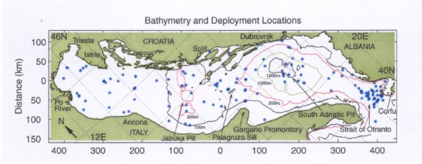
Figure 1:

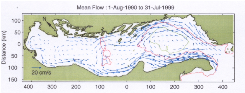
Figure 1:

Figure 2:

Figure 3:

Figure 4:

Figure 5:

Figure 5:

Figure 6:

Figure 6:

Figure 6:

Figure 7:

Figure 7:

Figure 8:

Figure 8:

Figure 9:

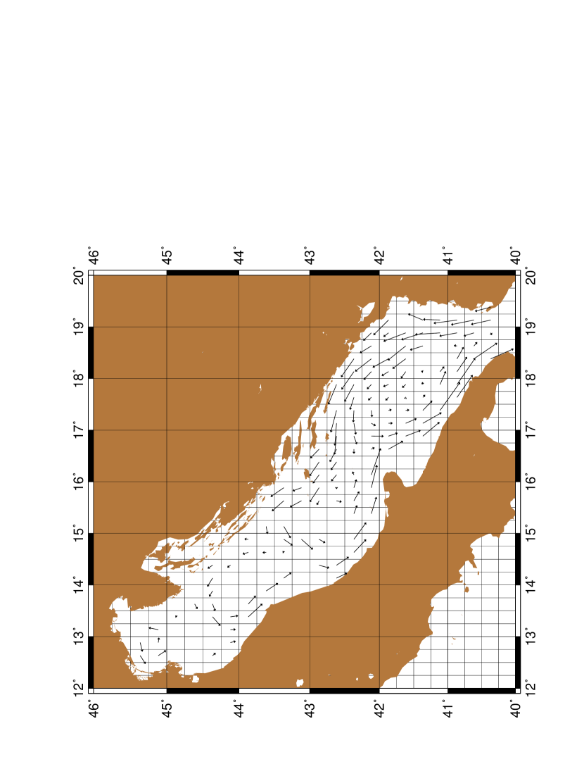
Figure 9:

Figure 10:

Figure 10:

References

- Artegiani et al., (1997) Artegiani, A., D. Bregant, E. Paschini, N. Pinardi, F. Raicich, and A. Russo, 1997: The Adriatic Sea general circulation, part II: Baroclinic circulation structure. J. Phys. Oceanogr., 27, 1515–1532.
- Batchelor, (1970) Batchelor, G., 1970: The theory of homogeneous turbulence, Cambridge University Press.
- Bauer et al., (2002) Bauer, S., M. Swenson, and A. Griffa, 2002: Eddy-mean flow decomposition and eddy-diffusivity estimates in the tropical pacific ocean. part 2: Results. J. Geophys. Res., 107, 3154–3171.
- Bauer et al., (1998) Bauer, S., M. Swenson, A. Griffa, A. Mariano, and K. Owens, 1998: Eddy-mean flow decomposition and eddy-diffusivity estimates in the tropical pacific ocean. part 1: Methodology. J. Geophys. Res., 103, 30,855–30,871.
- Berloff and McWilliams, (2002) Berloff, P. and McWilliams, 2002: Material transport in oceanic gyres. part ii: Hierarchy of stochastic models. J. Phys. Oceanogr., 32, 797–830.
- Bracco et al., (2000) Bracco, A., J. LaCasce, and A. Provenzale, 2000: Velocity pdfs for oceanic floats. J. Phys. Oceanogr., 30, 461–474.
- Castellari et al., (2001) Castellari, S., A. Griffa, T. Ozgokmen, and P.-M. Poulain, 2001: Prediction of particle trajectories in the Adriatic Sea using lagrangian data assimilation. J. Mar. Sys., 29, 33–50.
- Cerovecki et al., (1991) Cerovecki, I., Z. Pasaric, M. Kuzmic, J. Brana, and M. Orlic, 1991: Ten-day variability of the summer circulation in the North Adriatic. Geofizika, 8, 67–81.
- Corrsin, (1974) Corrsin, S., 1974: Limitation of gradient transport models in random walks and in turbulence. Annales Geophysicae, 18A, 25–60.
- Cushman-Roisin et al., (2001) Cushman-Roisin, B., M. Gacic, P.-M. Poulain, and A. Artegiani, 2001: Physical oceanography of the Adriatic Sea: Past, present and future, Kluwer Academic Publishers, 316 pp.
- Davis, (1987) Davis, R., 1987: Modelling eddy transport of passive tracers. J. Mar. Res., 45, 635–666.
- Davis, (1991) Davis, R., 1991: Observing the general circulation with floats. Deep-Sea Research, 38, S531–S571.
- Davis, (1994) Davis, R., 1994: Lagrangian and eulerian measurements of ocean transport processes, Ocean Processes in climate dynamics: Global and Mediterranean examples, P. Malanotte-Rizzoli and A. R. Robinson, eds., Eds., Kluwer Academic Publishers, pp. 29–60.
- Durst et al., (1987) Durst, F., J. Jovanovic, and L. Kanevce, 1987: Probability density distributions in turbulent wall boundary-layer flow, Turbulent Shear Flow 5, F. Durst, B. E. Launder, J. L. Lumley, F. W. Schmidt, and J. H. Whitelaw, eds., Springer, pp. 197–220.
- Falco et al., (2000) Falco, P., A. Griffa, P.-M. Poulain, and A. Zambianchi, 2000: Transport properties in the Adriatic Sea as deduced from drifter data. J. Phys. Oceanogr., 30, 2055–2071.
- Griffa, (1996) Griffa, A., 1996: Applications of stochastic particle models to oceanographic problems, Stochastic Modelling in Physical Oceanography, P. M. R.J. Adler and B. Rozovskii, eds., Birkhauser, pp. 114–140.
- Inoue, (1986) Inoue, 1986: A least square smooth fitting for irregularly spaced data: Finite element approach using the cubic -spline. Geophysics, 51, 2051–2066.
- Lenschow et al., (1994) Lenschow, D. H., J. Mann, and L. Kristensen, 1994: How long is long enough when measuring fluxes and other turbulence statistics? J. Atmos. Ocean. Technol., 11, 661–673.
- Maurizi and Lorenzani, (2001) Maurizi, A. and S. Lorenzani, 2001: Lagrangian time scales in inhomogeneous non-Gaussian turbulence. Flow, Turbulence and Combustion, 67, 205–216.
- Niiler et al., (1995) Niiler, P. P., A. S. Sybrandy, K. Bi, P.-M. Poulain, and D. S. Bitterman, 1995: Measurements of the water following capability of holey- and tristar drifters. Deep-Sea Research, 42, 1951–1964.
- Pasquero et al., (2001) Pasquero, C., A. Provenzale, and A. Babiano, 2001: Parameterization of dispersion in two-dimensional turbulence. J. Fluid Mech., 439, 278–303.
- Poulain, (1999) Poulain, P.-M., 1999: Drifter observations of surface circulation in the Adriatic Sea between december 1994 and march 1996. J. Mar. Sys., 20, 231–253.
- Poulain, (2001) Poulain, P.-M., 2001: Adriatic Sea surface circulation as derived from drifter data between 1990 and 1999. J. Mar. Sys., 29, 3–32.
- Poulain and Cushman-Roisin, (2001) Poulain, P.-M. and B. Cushman-Roisin, 2001: Chap. 3: Circulation, Physical oceanography of the Adriatic Sea: Past, present and future, B. Cushman-Roisin, M. Gacic, P.-M. Poulain, and A. Artegiani, eds., Kluwer Academic Publishers, pp. 67–109.
- Poulain et al., (2003) Poulain, P.-M., E. Mauri, C. Fayos, L. Ursella, and P. Zanasca, 2003: Mediterranean surface drifter measurements between 1986 and 1999, Tech. Rep. CD-ROM, OGS, in preparation.
- Poulain and Raicich, (2001) Poulain, P.-M. and F. Raicich, 2001: Chap. 2: Forcings, Physical oceanography of the Adriatic Sea: Past, present and future, B. Cushman-Roisin, M. Gacic, P.-M. Poulain, and A. Artegiani, eds., Kluwer Academic Publishers, pp. 45–65.
- Poulain and Zanasca, (1998) Poulain, P.-M. and P. Zanasca, 1998: Drifter observations in the Adriatic Sea (1994-1996) - data report, Tech. Rep. SACLANTCEN Memorandum SM-340, SACLANT Undersea Research Centre, La Spezia, Italy, 46 pp.
- Press et al., (1992) Press, W. H., S. A. Teukolsky, W. T. Vetterling, and B. P. Flannery, 1992: Numerical Recipes in FORTRAN, 2nd ed., Cambridge University Press.
- Priestley, (1981) Priestley, M., 1981: Spectral Analysis and Time Series, Academic Press, London, 890 pp.
- Raicich, (1996) Raicich, F., 1996: On the fresh water balance of the Adriatic Sea. J. Mar. Sys., 9, 305–319.
- Risken, (1989) Risken, H., 1989: The Fokker-Planck Equation: Methods of solutions and applications, Springer-Verlag, Berlin, 472 pp.
- Sawford, (1999) Sawford, B. L., 1999: Rotation of trajectories in Lagrangian stochastic models of turbulent dispersion. Boundary-Layer Meteorol., 93, 411–424.
- Swenson and Niiler, (1996) Swenson, M. and P. Niiler, 1996: Statistical analysis of the surface circulation of the California current. J. Geophys. Res., 101, 22,631.
- Thomson, (1987) Thomson, D., 1987: Criteria for the selection of stochastic models of particle trajectories in turbulent flows. J. Fluid Mech., 180, 529–556.
- Veneziani et al., (2003) Veneziani, M., A. Griffa, A. Reynolds, and A. Mariano, 2003: Oceanic turbulence and stochastic models from subsurface lagrangian data for the north-west atlantic ocean. J. Phys. Oceanogr., submitted.
- Zhang et al., (2001) Zhang, H., M. Prater, and T. Rossby, 2001: Isopycnal lagrangian statistics from the North Atlantic Current RAFOS floats observations. J. Geophys. Res., 106, 13,187–13,836.