Spatially Differential Forms of Lenz Law

Abstract

Two sets of spatially differential formulas of Lenz law on electromagnetic inductance are presented. They are a cut-magnetic flux induced voltage, which instantaneously results from cutting magnetic flux as a conductor moving with respect to an external magnetic field, and a wave-induced voltage due to the interaction of a conductor or charged particles with the arriving electromagnetic wave, which is originated from a changing magnetic flux source. Upon the Lenz differential forms, the induced electrical field strength, relevant properties and their application are discussed.

Lenz law, as an empirical rule, sums production and property of inductive electromotive force in a conductor loop when an interaction occurs between the circle loop and a steady magnetic field or changeable magnetic field. It is expressed in an integral formula of induced electromotive voltage on whole conductor loop and can be applied for a totally induced electrical voltage calculation in steady-symmetric circumstances Gray and Isaacs (1975),

$$\varepsilon_{t}(t)=\oint{\boldsymbol{E}_{t}(t)\cdot\mathrm{d}\boldsymbol{l}}=-\oint_{\ell}{\delta\mathit{\dot{\Phi}}_{t}(t)}\;.$$ (1)

However in physical practice there are variety of induction phenomena which occur in a non-steady status with asymmetric circumstances; or the induced electrical strength are needed to be calculated upon an interestedly particular point, segment of conductor on differently spatial condition as such where the integral form Eq.(1) can not be in use Luo (2000, 2003). Moreover the integrated form will cover some explicit details of physical properties that can be revealed and applied through its spatially differential forms. Like the important role of Biot-Savart theorem (or differential form of Ampere theorem) on magnetic field calculation[ Gray and Isaacs (1975); Bueche (1975), therefore, the presentation of the differential form of Lenz law will be significant to time-dependent calculation of induced electrical field.

Actually electromagnetic inductances occur on a spatial conductor element or charged particles much more often than on a whole conductor loop. Mathematically the integral form is merely an accumulated sum of spatial differential inductance results along the whole loop. And in viewpoint of physics, the causes of all electromagnetic inductance phenomena could be divided into two categories: cut-magnetic flux induced electrical field and wave-induced electrical field. The integral form is given as

$$\begin{split}\varepsilon_{t}(t)&=\oint{\boldsymbol{E}_{\mathrm{c}}(t)\cdot\mathrm{d}\boldsymbol{l}}-\oint{\boldsymbol{E}_{w}(t)\cdot\mathrm{d}\boldsymbol{l}}\\ &=-\left[{\oint{\delta\mathit{\dot{\Phi}}_{d\ell c}(t)}+\oint{\delta\mathit{\dot{\Phi}}_{d\ell w}(t)}}\right]\\ &=-\oint{\delta\left[{\mathit{\dot{\Phi}}_{d\ell c}(t)+\mathit{\dot{\Phi}}_{d\ell w}(t)}\right]}\;.\\ \end{split}$$ (2)

Upon Eq.(2), for having differently physical properties the cut-magnetic flux induced field and wave-induced field on the conductor are classified into two categories. The former is related to energy conversion from mechanical kinetic energy to electrical energy, and the latter related to the conversion from an electromagnetic wave kinetic energy to an associated energy carried or possessed by a conductor or charged particles.

The spatial differential Form of the cut-magnetic field induced voltage can be given below,

$$\begin{split}d\varepsilon_{c}(t)&=-\left[{\boldsymbol{v}_{d\ell\cdot b}(t)\times\boldsymbol{B}(t)}\right]\cdot\mathrm{d}\boldsymbol{l}\\ &=-\boldsymbol{E}_{c}(t)\cdot\mathrm{d}\boldsymbol{l}\\ &=-\delta\mathit{\dot{\Phi}}_{d\ell c}(t)\;.\\ \end{split}$$ (3)

Where: $-\frac{\pi}{2}\leqslant\alpha_{c}=\widehat{\boldsymbol{n}_{\kern-1.39998pt\lower 0.90417pt\hbox{$\scriptscriptstyle{\boldsymbol{E}}_{c}$}}\!(t)\boldsymbol{n}_{d\boldsymbol{l}}(t)}\leqslant\tfrac{\pi}{2}$, $0\leqslant\delta\mathit{\dot{\Phi}}_{d\ell c}(t)=\boldsymbol{E}_{c}(t)\cdot\boldsymbol{n}_{dl}(t)d\ell$.

$\boldsymbol{v}_{d\ell\cdot b}(t)$ — relative velocity of conductor element $d\boldsymbol{l}$ with respect to $\boldsymbol{B}(t)$, $\boldsymbol{v}_{d\ell\cdot b}=\boldsymbol{v}_{d\ell}-\boldsymbol{v}_{b}$;

$\boldsymbol{E}_{c}(t)$ — induced electrical field strength in conductor element by cutting magnetic flux; or induced electrical force per unit length along $\boldsymbol{v}_{d\ell\cdot b}(t)\times\boldsymbol{B}(t)$ direction by cutting $\boldsymbol{B}(t)$ field.

As conductor element $d\boldsymbol{l}$ moves in external magnetic field the Lorentz action will cause an energy conversion from a non-electrical energy (such as kinetic energy) to an electrical energy. It is the action that results in an induced electrical field strength $\boldsymbol{E}_{c}(t)$ inside of the conductor, or an elemental induced electromotive force or voltage $d\varepsilon_{c}(t)$ in conductor, its value depends upon induced electrical field strength, and size and orientation of the conductor. The derivation is following:

$$\begin{split}d\varepsilon_{d\ell c}\left[{\boldsymbol{r}(t)}\right]&=-B\left[{\boldsymbol{r}(t)}\right]A_{c\bot b}(t)=-Bv_{\bot}d\ell_{{}_{//\boldsymbol{v}\times\boldsymbol{B}}}=-Bv_{{}_{d\ell\cdot b}}\sin\theta_{c}d\ell\cos\alpha_{c}\\ &=\boldsymbol{B}(t)\cdot\left\{{\left[{\boldsymbol{v}_{d\ell\cdot b}(t)\times\boldsymbol{n}_{b}(t)}\right]\times\left[{d\boldsymbol{l}\times\boldsymbol{n}_{b}(t)}\right]}\right\}\\ &=-B(t)\left[{\boldsymbol{n}_{b}(t)\times d\boldsymbol{l}}\right]\cdot\left\{{\boldsymbol{n}_{b}(t)\times\left[{\boldsymbol{v}_{d\ell\cdot b}(t)\times\boldsymbol{n}_{b}(t)}\right]}\right\}\\ &=-B(t)\left[{\boldsymbol{n}_{b}(t)\times d\boldsymbol{l}}\right]\cdot\left\{{\left[{\boldsymbol{n}_{b}(t)\cdot\boldsymbol{n}_{b}(t)}\right]\boldsymbol{v}_{d\ell\cdot b}(t)-\left[{\boldsymbol{n}_{b}(t)\cdot\boldsymbol{v}_{d\ell\cdot b}(t)}\right]\boldsymbol{n}_{b}(t)}\right\}\\ &=-B(t)\left[{\boldsymbol{n}_{b}(t)\times d\boldsymbol{l}}\right]\cdot\left\{{\boldsymbol{v}_{d\ell\cdot b}(t)-\left[{\boldsymbol{n}_{b}(t)\cdot\boldsymbol{v}_{d\ell\cdot b}(t)}\right]\boldsymbol{n}_{b}(t)}\right\}\\ &=-B(t)d\boldsymbol{l}\cdot\left\{{\left\{{\boldsymbol{v}_{d\ell\cdot b}(t)-\left[{\boldsymbol{n}_{b}(t)\cdot\boldsymbol{v}_{d\ell\cdot b}(t)}\right]\boldsymbol{n}_{b}(t)}\right\}\times\boldsymbol{n}_{b}(t)}\right\}\\ &=-B(t)\left[{\boldsymbol{v}_{d\ell\cdot b}(t)\times\boldsymbol{n}_{b}(t)}\right]\cdot d\boldsymbol{l}\\ &=-\left[{\boldsymbol{v}_{d\ell\cdot b}(t)\times\boldsymbol{B}(t)}\right]\cdot\boldsymbol{n}_{d\boldsymbol{l}}(t)d\ell\\ &=-\boldsymbol{E}_{c}(t)\cdot\boldsymbol{n}_{d\boldsymbol{l}}(t)d\ell\\ &=-\delta\mathit{\dot{\Phi}}_{d\ell c}(t)\;.\\ \end{split}$$ (4)

Here $\theta_{c}$: the angle between the direction of the magnetic flux density at the conductor location and that of $bs{v}_{d\ell\cdot b}(t)$ or $\theta_{c}=\widehat{\boldsymbol{n}(\boldsymbol{v}_{d\ell\cdot b})\boldsymbol{n}_{b}}$ and

$$\boldsymbol{E}_{c}(t)=\boldsymbol{v}_{d\ell\cdot b}(t)\times\boldsymbol{B}(t)=v_{{}_{d\ell\cdot b}}B\sin\theta_{c}\boldsymbol{n}(\boldsymbol{v}_{d\ell\cdot b}\times\boldsymbol{B})\;.$$ (5)

Take an integrated form of Eq.(4) there exists

$$\begin{split}\varepsilon_{c}(t)&=\oint_{\ell}{d\varepsilon_{d\ell c}(t)}\\ &=-\oint_{\ell}{\left[{\boldsymbol{v}_{d\ell\cdot b}(t)\times\boldsymbol{B}(t)}\right]\cdot\mathrm{d}\boldsymbol{l}}\\ &=-\oint_{\ell}{\boldsymbol{E}_{c}(t)\cdot\mathrm{d}\boldsymbol{l}}\\ &=-\oint_{\ell}{\delta\mathit{\dot{\Phi}}_{d\ell c}(t)}\;.\\ \end{split}$$ (6)

Eq.(5,6) reveal that at spatially different points of the conductor, Lorentz action exerted on the positive and negative charges within the conductor, the separately electromotive force in the opposite directions, is the only cause to form the cut-induced electrical field within a conductor.

Another type of electromagnetic inductance results from the interaction of the conductor or charged particles as electromagnetic load with the arriving electromagnetic wave. The energy of the electromagnetic radiation, originated from a changing magnetic flux source or a source of magnetic flux rate, will induce an associated electrical field at the conductor location and be transferred into an associated energy of the conductor or charged particles in their overlapped space.

$$\begin{split}\boldsymbol{E}_{sw}({t}^{\prime})&=\boldsymbol{E}_{sw}({t}^{\prime}=t+T)\\ &=\frac{\boldsymbol{n}(\boldsymbol{r}_{sd\ell})\times\boldsymbol{n}_{b}\dot{B}\left[{\boldsymbol{r}_{s}(t)}\right]ds_{\bot b}dL}{4\pi r_{sd\ell}^{2}}\\ &=\frac{\boldsymbol{n}(\boldsymbol{r}_{sd\ell})\times\boldsymbol{n}_{b}\delta\mathit{\dot{\Phi}}_{w}(t)dL}{4\pi r_{sd\ell}^{2}}\\ &=\frac{\boldsymbol{n}(\boldsymbol{r}_{sd\ell})\times\dot{\boldsymbol{B}}\left[{\boldsymbol{r}_{s}(t)}\right]dV}{4\pi r_{sd\ell}^{2}}\\ &=\frac{\boldsymbol{n}(\boldsymbol{r}_{sd\ell})\times\delta\dot{\boldsymbol{M}}(t)}{4\pi r_{sd\ell}^{2}}\\ &=\frac{\dot{B}\left[\boldsymbol{r}_{s}(t)\right]dVsin\theta(t)}{4\pi r^{2}_{sd\ell}}\boldsymbol{n}\left[\boldsymbol{n}(\boldsymbol{r}_{sd\ell})\times\boldsymbol{n}_{b}\right]\\ &=E_{w}(t^{\prime})\boldsymbol{n}_{{}_{\boldsymbol{E}_{w}}}(t^{\prime})\;,\end{split}$$ (7)

where, $\boldsymbol{E}_{sw}(t^{\prime})$ — the induced electrical field strength, or induced electrical force per unit length on a conductor along $\boldsymbol{n}(\boldsymbol{r}_{sd\ell})\times\delta\dot{\boldsymbol{M}}(t)$ direction by electromagnetic wave originated from a micro magnetic flux rate element $\delta\dot{\boldsymbol{M}}(t)$ in an air and vacuum space;
$\delta\dot{\boldsymbol{M}}=\dot{\boldsymbol{B}}\left[{\boldsymbol{r}_{s}(t)}\right]dV=\boldsymbol{n}_{b}\delta\mathit{\dot{\Phi}}_{w}(t)dL=\boldsymbol{n}_{b}\dot{B}\left[{\boldsymbol{r}_{s}(t)}\right]ds_{\bot b}dL$ — a spatial element of magnetic flux’s rate;
$\boldsymbol{n}_{b}$ — the unit vector of magnetic flux density $\boldsymbol{B}\left[{\boldsymbol{r}_{s}(t)}\right]$ at $t$ instant and $\boldsymbol{r}_{s}(t)$position;
$\theta_{w}$ — the angle between the direction of $\boldsymbol{B}[\boldsymbol{r}_{s}(t)]$ and that of the relative position vector $\boldsymbol{r}_{sd\ell}$;
$\boldsymbol{n}\left[\boldsymbol{n}(\boldsymbol{r}_{sd\ell})\times\boldsymbol{n}_{b}\right]=\boldsymbol{n}\left[\boldsymbol{n}(\boldsymbol{r}_{sd\ell})\times\delta\dot{\boldsymbol{M}}(t)\right]=\boldsymbol{n}_{{}_{\boldsymbol{E}_{w}}}(t^{\prime})$ in an air and vacuum space;
$0\leqslant\alpha_{w}=\widehat{\boldsymbol{n}_{{}_{\boldsymbol{E}_{w}}}({t}^{\prime})\boldsymbol{n}_{d\boldsymbol{l}}({t}^{\prime})}\leqslant{\pi}$, $0\leqslant\delta\mathit{\dot{\Phi}}_{d\ell w}({t}^{\prime})=\boldsymbol{E}_{w}({t}^{\prime})\cdot\boldsymbol{n}_{d\boldsymbol{l}}({t}^{\prime})d\ell$;
$\boldsymbol{r}_{sd\ell}=r_{sd\ell}\boldsymbol{n}(\boldsymbol{r}_{sd\ell})$ — relative position vector between a micro magnetic flux’s rate spatial element $\delta\dot{\boldsymbol{M}}=\dot{\boldsymbol{B}}\left[{\boldsymbol{r}_{s}(t)}\right]dV$ and a micro conductor element $d\boldsymbol{l}$;
$t$, ${t}^{\prime}$ — emitting instant and arriving instant respectively of a micro electromagnetic wave element originated from the magnetic flux’s rate source, here ${t}^{\prime}-t=T(t)=T({t}^{\prime})$.

So the generally spatial differential form of the wave-induced voltage will be given below,

$$\begin{split}d\varepsilon_{w}({t}^{\prime})&=-\left[{\sum{\boldsymbol{E}_{jsw}({t}^{\prime})}}\right]\cdot d\boldsymbol{l}\\ &=-\left[{\sum{\frac{\boldsymbol{n}(\boldsymbol{r}_{jsd\ell})\times\boldsymbol{n}_{b}\delta\mathit{\dot{\Phi}}_{jw}(t_{j})dL_{j}}{4\pi r_{jsd\ell}^{2}}}}\right]\cdot d\boldsymbol{l}\\ &=-\left[{\sum{\frac{\boldsymbol{n}(\boldsymbol{r}_{jsd\ell})\times\dot{\boldsymbol{B}}\left[{\boldsymbol{r}_{js}(t_{j})}\right]dV_{j}}{4\pi r_{jsd\ell}^{2}}}}\right]\cdot d\boldsymbol{l}\\ &=-\left[{\sum{\frac{\boldsymbol{n}(\boldsymbol{r}_{jsd\ell})\times\delta\dot{\boldsymbol{M}}_{j}(t_{j})}{4\pi r_{jsd\ell}^{2}}}}\right]\cdot d\boldsymbol{l}\\ &=-\boldsymbol{E}_{w}({t}^{\prime})\cdot d\boldsymbol{l}\\ &=-\delta\mathit{\dot{\Phi}}_{d\ell w}\left[{\boldsymbol{r}_{d\ell}({t}^{\prime})}\right]\;.\end{split}$$ (8)

Eq.(7,8) manifest a general explicitly formula of purely wave-induced electrical field strength at a detector position where the charged particles or a conductor serve as a electromagnetic load to interact with an arriving electromagnetic wave. In the process an energy exchange will occur among the electromagnetic energy possessed by the load and wave respectively. It is known that the associated induced electrical strength is related to spatial propagating distribution, attenuation and time delay of the wave-energy.

For a steady wave-induction circumstance, the induced voltage element can be expressed:

$$\begin{split}d\varepsilon_{w}({t}^{\prime})&=-\boldsymbol{E}_{w}({t}^{\prime})\cdot d\boldsymbol{l}\\ &=-\left[\iiint_{\dot{M}}{\frac{\boldsymbol{n}(\boldsymbol{r}_{sd\ell})\times\delta\dot{\boldsymbol{M}}(t)}{4\pi r_{sd\ell}^{2}}}\right]\cdot d\boldsymbol{l}\\ &=-\left[\iiint_{V}{\frac{\boldsymbol{n}(\boldsymbol{r}_{sd\ell})\times\dot{\boldsymbol{B}}(t)\mathrm{d}V}{4\pi r_{sd\ell}^{2}}}\right]\cdot d\boldsymbol{l}\;.\end{split}$$ (9)

Or when the spatial shape of the magnetic flux’s rate source is long tube like shape with small cross section area $ds_{\bot b}$ usually taken in practical cases, then the induced electrical force can be expressed as:

$$\begin{split}\boldsymbol{E}_{w}({t}^{\prime})&=\iiint_{\dot{M}}{\frac{\boldsymbol{n}(\boldsymbol{r}_{sd\ell})\times\delta\dot{\boldsymbol{M}}(t)}{4\pi r_{sd\ell}^{2}}}\\ &=\iiint_{V}{\frac{\boldsymbol{n}(\boldsymbol{r}_{sd\ell})\times\dot{\boldsymbol{B}}(t)\mathrm{d}V}{4\pi r_{sd\ell}^{2}}}\\ &=\int_{L}{\iint_{ds}{\frac{\boldsymbol{n}(\boldsymbol{r}_{sd\ell})\times\boldsymbol{n}_{b}\dot{B}(t)\mathrm{d}s_{\bot b}}{4\pi r_{sd\ell}^{2}}}}\mathrm{d}L\\ &=\int_{L}{\frac{\boldsymbol{n}(\boldsymbol{r}_{sd\ell})\times\boldsymbol{n}_{b}\delta\mathit{\dot{\Phi}}(t)}{4\pi r_{sd\ell}^{2}}}\mathrm{d}L\;.\end{split}$$ (10)

Following is an illustrating example of calculating wave-induced electrical field strength in steady-symmetry circumstance (Ref. Fig. 1).

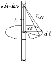
Figure 1: Diagram of wave-induced electrical field by a micro magnetic flux rate element

Take an integral form of Eq.(10), there then exists

$$\begin{split}\boldsymbol{E}_{w}({t}^{\prime})&=\iiint_{\dot{M}}{\frac{\boldsymbol{n}(\boldsymbol{r}_{sd\ell})\times\delta\dot{\boldsymbol{M}}({t}^{\prime})}{4\pi r_{sd\ell}^{2}}}\\ &=\iiint_{V}{\frac{\boldsymbol{n}(\boldsymbol{r}_{sd\ell})\times\dot{\boldsymbol{B}}t({t}^{\prime})\mathrm{d}V}{4\pi r_{sd\ell}^{2}}}\\ &=\int_{L}{\frac{\boldsymbol{n}(\boldsymbol{r}_{sd\ell})\times\dot{B}\left({t}^{\prime}\right)ds_{\bot b}\boldsymbol{n}_{b}\mathrm{d}L}{4\pi r_{sd\ell}^{2}}}\\ &=\int_{0}^{\infty}{\frac{2r_{0}\delta\mathit{\dot{\Phi}}({t}^{\prime})\boldsymbol{n}_{\kern-1.39998pt\lower 0.90417pt\hbox{$\scriptscriptstyle{\boldsymbol{E}}_{w}$}}}{4\pi(r_{0}^{2}+L^{2})^{\raise 1.50694pt\hbox{$\scriptstyle 3$}\kern-0.70004pt/\kern-1.04996pt\lower 0.75346pt\hbox{$\scriptstyle 2$}}}\mathrm{d}L}\\ &=\frac{\delta\mathit{\dot{\Phi}}({t}^{\prime})}{2\pi r_{0}}\boldsymbol{n}_{\kern-1.39998pt\lower 0.90417pt\hbox{$\scriptscriptstyle{\boldsymbol{E}}_{w}$}}=E_{w}({t}^{\prime})\boldsymbol{n}_{\kern-1.39998pt\lower 0.90417pt\hbox{$\scriptscriptstyle{\boldsymbol{E}}_{w}$}}\;,\\ \end{split}$$ (11)

it is $\left|{\boldsymbol{E}_{w}({t}^{\prime})}\right|=\tfrac{\delta\mathit{\dot{\Phi}}({t}^{\prime})}{2\pi r_{0}}$. So

$$\begin{split}\varepsilon_{w}({t}^{\prime})&=\oint_{\ell}{E_{w}({t}^{\prime})\boldsymbol{n}_{\kern-1.39998pt\lower 0.90417pt\hbox{$\scriptscriptstyle{\boldsymbol{E}}_{w}$}}\cdot\mathrm{d}\boldsymbol{l}}=\oint_{\ell}{\frac{\delta\mathit{\dot{\Phi}}({t}^{\prime})}{2\pi r_{0}}\boldsymbol{n}_{\kern-1.39998pt\lower 0.90417pt\hbox{$\scriptscriptstyle{\boldsymbol{E}}_{w}$}}\cdot\mathrm{d}\boldsymbol{l}}\\ &=-\oint_{\ell}{\frac{\delta\mathit{\dot{\Phi}}({t}^{\prime})}{2\pi r_{0}}\mathrm{d}\ell=-\int_{0}^{2\pi}{\frac{\delta\mathit{\dot{\Phi}}({t}^{\prime})}{2\pi}\mathrm{d}\theta}}\\ &=-\delta\mathit{\dot{\Phi}}({t}^{\prime})\;.\end{split}$$

Meanwhile by applying Eq.(1) in the case, the following equations can be derived.

$$\varepsilon_{w}({t}^{\prime})=\oint{d\varepsilon_{w}({t}^{\prime})=}\oint{E_{w}({t}^{\prime})\cdot d\ell}=2\pi r_{0}E_{w}({t}^{\prime})=-\delta\mathit{\dot{\Phi}}({t}^{\prime})\;,$$ (12)

and

$$\left|{\boldsymbol{E}_{w}({t}^{\prime})}\right|=\frac{\delta\mathit{\dot{\Phi}}({t}^{\prime})}{2\pi r_{0}}.$$ (13)

Eq.(11, 12) testifies that the calculated results are consistent by using any one among the differential form of wave-induced electrical field and Lenz integrated form along a closed circular loop in a steady-symmetry induction situation with even-radial electromagnetic radiant wave from center of the loop.

Combining the two types of inductance together, there are the consequences on the total inductance forms as following.

$$\begin{split}&\boldsymbol{E}_{t}({t}^{\prime})=\boldsymbol{E}_{c}({t}^{\prime})+\boldsymbol{E}_{w}({t}^{\prime})\\ &=\boldsymbol{v}_{d\ell\cdot b}({t}^{\prime})\times\boldsymbol{B}({t}^{\prime})+\sum{\frac{\boldsymbol{n}(\boldsymbol{r}_{jsd\ell})\times\delta\dot{\boldsymbol{M}}_{j}({t}^{\prime}-T_{j})}{4\pi r_{jsd\ell}^{2}}}\\ &=\boldsymbol{v}_{d\ell\cdot b}({t}^{\prime})\times\boldsymbol{B}({t}^{\prime})+\sum{\frac{\boldsymbol{n}(\boldsymbol{r}_{jsd\ell})\times\dot{\boldsymbol{B}}_{j}\left[{\boldsymbol{r}_{s}\left({{t}^{\prime}-T_{j}}\right)}\right]dV_{j}}{4\pi r_{jsd\ell}^{2}}}\;.\end{split}$$ (14)

For steady electromagnetic induction situation, an induced electrical strength at a point can be expressed as below,

$$\begin{split}\boldsymbol{E}_{t}({t}^{\prime})&=\boldsymbol{E}_{c}({t}^{\prime})+\boldsymbol{E}_{w}({t}^{\prime})\\ &=\boldsymbol{v}_{d\ell\cdot b}({t}^{\prime})\times\boldsymbol{B}({t}^{\prime})+\iiint_{\dot{M}}{\frac{\boldsymbol{n}(\boldsymbol{r}_{sd\ell})\times\delta\dot{\boldsymbol{M}}(\boldsymbol{r}_{s},{t}^{\prime})}{4\pi r_{sd\ell}^{2}}}\\ &=\boldsymbol{v}_{d\ell\cdot b}({t}^{\prime})\times\boldsymbol{B}({t}^{\prime})+\iiint_{V}{\frac{\boldsymbol{n}(\boldsymbol{r}_{sd\ell})\times\dot{\boldsymbol{B}}(\boldsymbol{r}_{s},{t}^{\prime})dV}{4\pi r_{sd\ell}^{2}}}\;.\end{split}$$ (15)

The total induced voltage on the conductor element is given then,

$$\begin{split}d\varepsilon_{t}({t}^{\prime})&=-\boldsymbol{E}_{t}({t}^{\prime})\cdot d\boldsymbol{l}\\ &=-\left[{\boldsymbol{E}_{c}({t}^{\prime})+\boldsymbol{E}_{w}({t}^{\prime})}\right]\cdot d\boldsymbol{l}\\ &=-\delta\left[{\mathit{\dot{\Phi}}_{d\ell c}({t}^{\prime})+\mathit{\dot{\Phi}}_{d\ell w}({t}^{\prime})}\right]\;.\end{split}$$ (16)

The spatial differential forms can be applied mainly to two aspects.

1. Calculation of induced electrical field strength will be conducted on any particular point, segment or non-closed loop of conductor with asymmetry circumstance where Lenz integral form can not be applied in purpose, such as the calculation of wave-induced electrical field strength at center point of a toroid source of changing magnetic flux; the calculation of wave-induced electrical field ($\boldsymbol{E}_{w})$ could be applied to a time-dependent spatial ($\boldsymbol{E}_{w})$ field distribution.

2. Explicit and quantitative analysis on the energy conversion, spatial orientation or polarization of induced electrical field strength on a conductor element and their time rate in a dynamic process of electromagnetic inductance. In addition, the time delay of the wave-induced signal, due to the wave propagating from the source of magnetic flux rate to the conductor element, can be analyzed upon the spatial differential form.

Lenz experimental law can be reduced to two fundamentally spatial differential forms: cut-magnetic field induced electrical field and wave-induced electrical field on a conductor element. In both cases a relative velocity between the conductor and a contact magnetic field or magnetic flux rate field is necessary preposition for inductance occurrence. The spatial differential forms not only manifest explicitly the physical essence of electromagnetic inductance but also can be applied as the calculating formulas in variety of calculation and analysis of electromagnetic inductance phenomena where Lenz integral form can not offer the relevant explicit solution as its mathematical limit.

References

• Gray and Isaacs (1975) H. J. Gray and A. Isaacs, A New Dictionary of Physics (Longman, New York, 1975), pp. 19–20,173–174.
• Luo (2000) J. Luo, Electromagnetic response of transmission line under short circuit by carbon-based fiber, Ph.D. Dissertation, Beijing Institute of Technology, Beijing (2000).
• Luo (2003) J. Luo, Energy differential structure and energy exchange of a micro element of charged particles in longintudinal acceleration, Postdoctoral Research Report, Institute of High Energy Physics, Chinese Academy of Sciences, Beijing (2003).
• Bueche (1975) F. J. Bueche, Introduction to physics for scientists and engineers (McGraw-Hill Book Company, New York, 1975), pp. 456–472, 475–497.